Modeling the effects of surface and bottom geometries on LiDAR bathymetric waveforms

HAL Id: hal-01523133

https://hal.archives-ouvertes.fr/hal-01523133

HAL is a multi-disciplinary open access

archive for the deposit and dissemination of sci-entific research documents, whether they are pub-lished or not. The documents may come from teaching and research institutions in France or abroad, or from public or private research centers.

L’archive ouverte pluridisciplinaire HAL, est destinée au dépôt et à la diffusion de documents scientifiques de niveau recherche, publiés ou non, émanant des établissements d’enseignement et de recherche français ou étrangers, des laboratoires publics ou privés.

Distributed under a Creative Commons Attribution - NonCommercial - ShareAlike| 4.0 International License

Modeling the effects of surface and bottom geometries

on LiDAR bathymetric waveforms

Martin Montes-Hugo, Jean-Stéphane Bailly, Nicolas Baghdadi, Anis

Bouhdaoui

To cite this version:

Martin Montes-Hugo, Jean-Stéphane Bailly, Nicolas Baghdadi, Anis Bouhdaoui. Modeling the effects of surface and bottom geometries on LiDAR bathymetric waveforms. Geoscience and Remote Sensing Symposium (IGARSS), 2014 IEEE International, IEEE International, Jul 2014, Quebec, Canada. pp.2706 - 2708, �10.1109/IGARSS.2014.6947033�. �hal-01523133�

MODELING THE EFFECTS OF SURFACE AND BOTTOM GEOMETRIES ON LIDAR

BATHYMETRIC WAVEFORMS

Martin Alejandro Montes-Hugo1_{, Jean-Stéphane Bailly}2,3_{, Nicolas Baghdadi}4_{, Anis Bouhdaoui}4,5

1_{ISMER, UQAR, Rimouski Québec, Canada}

2_{AgroParisTech, UMR TETIS, F-34093 Montpellier, France} 3_{AgroParisTech, UMR LISAH, F-34060 Montpellier, France}

4_{IRSTEA, UMR TETIS, F-34093 Montpellier, France} 5_{Ecole Polytechnique, LMD, F-91128 Palaiseau, France}

ABSTRACT

LiDAR bathymetric biases due to geometric changes at the air-water and water-bottom interfaces are investigated based on calculations made with a modified version of the waveform simulator Wa-LID. Main assumptions include a homogeneous water column and a spaceborne Lidar with a wavelength centered at 532 nm. Preliminary results showed major temporal modifications on second Lidar return (up to

± 100 cm or ± 10 ns) due to tilted bottoms. This shift was in average >6-fold the maximum bottom depth bias originated from capillary waves forming at the air-water surface.

Index Terms— Lidar, bathymetry, model, surface effects,

bottom

1. INTRODUCTION

LiDAR (Light Detection And Ranging) bathymetry is usually retrieved using the positions of the air-water interface and the water bottom backscattered pulses derived from a green LiDAR waveform. For an optical opaque media, such as bare soils or building materials, the waveform shape is known to be sensitive to the surface slope or roughness of the media, i.e. the geometry of the surface within the laser beam footprint [1].

The main geometric influence of boundaries (air-water and water-bottom) on LiDAR waveforms is the effect of pulse stretching [2]. Several analytical formulations were proposed to explain the pulse stretching as a function of the target slope [2,3]. Empirical studies on the accuracy of LiDAR airborne bathymetry [4,5] often report observed biases, i.e., a systematic underestimation of the bathymetry estimates. However, the explanations of the exact causes of these biases are few and vary among studies, most likely because of the lack of highly detailed reference data on the

target properties at the airborne footprint scale that can help researchers better understand these causes.

In this study, we hypothesize that LiDAR bathymetric biases and underestimations are principally originated from geometric changes at the air-water and water-bottom interfaces due to a temporal shift and associated stretching of the LiDAR signal. In this study, we aimed to test these effects using an extended bathymetric LiDAR waveform simulator Wa-LID [6]. Extensions within the existing simple analytical Wa-LID model [6] include i) an analytical module for modeling the geometry of the water-bottom interface in 1-D [7], and ii) a stochastic module to parameterize the rugosity of the air-water interface and based on Monte Carlo realizations of mean slopes for capillary waves [8, 9, 10]. This analysis was performed considering a wide simulated LiDAR footprint (<50 m) representative of future sapceborne LiDAR bathymetric satellite sensors (e.g., EADS-Astrium).

2. METHODS

This theoretical study is using a waveform simulator that was specifically designed to take into account different air-water boundaries, air-water properties, and bottom morphologies. Multiple simulated waveforms assuming boundaries (air-water and water-bottom) with different geometries allow to quantify the contribution of each interface to the bathymetry error. In all cases, the bottom depth is computed from the waveform as the time difference between the surface peak at the air-water interface and the bottom return [11]. For the sake of simplicity, only results related to the bottom geometry are presented here.

2.1. Modeled water-bottom interface

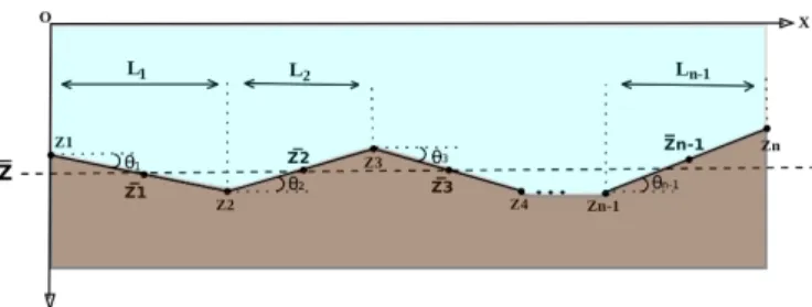
First, we propose a simplified 1D geometric model for the water-bottom boundary as a succession of n-1 contiguous segments with n endpoints denoted Zi [7]. Each segment is

on the X-axis and a slope angle θi with respect to the X-axis

(Fig. 1).

Figure 1. Simplified 1D water bottom geometry along the footprint diameter (X axis) having bathymetry

_z

Although a simplification, the 1D bottom geometry is appropriate for demonstrating the first order impact of the bottom geometry on bottom depth estimation. Another approximation was the use of a discretization scheme for.simulating a continuous bottom. First, the segments describing the water bottom geometry are spatially defined along the X-axis into m samples with the spatial lag δx. At a given sample xf along the X-axis with a water depth of Zf,

a waveform denoted Pbf(t) with a footprint diameter of Fp is

simulated using the Wa-LID simulator [6], where the water bottom is assumed to be a Lambertian reflector [12]. We assumed that illuminating a non-flat bottom can be approached by illuminating a staircase function with a δx spatial lag. Consequently, the resulting simulated waveform Pb(t) at the footprint scale, considering the complex water

bottom geometry, is computed by weight averaging the waveforms Pbf(t) and accounting for the Gaussian beam

profile:

P

(

t

)

=

∑

w

P

(

t

)

2.2. Modeled air-water interface

Variability of LiDAR refracted angles (vertical and horizontal components) due to capillary waves are investigated based on Monte Carlo simulations of wave slope components (i.e., along and across) calculated as a function of the average wind speed 10 m above the sea surface and the Richardson number, an index of air-sea instability [8,9,10]. For a specific sea state, slope contributions are modified based on random probabilities extracted from cumulative distribution functions based on Gaussian functions having an arithmetic mean equal to zero and a variance equal to 1 [9].

2.3 .Experimental design for bathymetry accuracy estimation

LiDAR waveform simulations were performed using an optically homogeneous water column and a LiDAR system

configuration involving spaceborne measurements [7]. In the simulations, a green Nd:Yag laser wavelength (532 nm) was used. This wavelength minimizes the attenuation of the bottom return due to water absorption. To examine the effect of bottom geometry on accuracy of bottom depth retrievals, simulations were conducted using a bottom depth of 2, 5, 8, and 12 m. Bottom geometries were constructed with 3 segments having a slope angle varying between 0 and 30 degrees. Four case studies were proposed where each angle corresponds to the first vertex of each segment : 'flat' (0°:0°:0°), 'zig-zag' (-30°:30°:-30°), 'valley' (0°:-30°:30°) and 'hill' (0°:30°:0°). Notice that negative and positive angles are clockwise and anticlockwise with respect to the horizontal (i.e., X-axis), respectively. To retrieve the bathymetry from each waveform, a simple waveform peak detection method based on the local maximum was used. The first peak in the temporal sequence is usually the LiDAR return at the air-water interface. Conversely, the bottom LiDAR return is delayed and is assigned to the second largest peak observed in the waveform.

3. RESULTS AND DISCUSSION

To highlight the influence of the bottom geometry on the shape of the LiDAR waveforms, Figure 2 shows five weighted waveforms using different configurations of slope angles of three successive 1.6 meter length segments that describe the geometry of the water bottom.

4. TYPE-STYLE AND FONTS

Figure 2. Example of five simulated LiDAR waveforms with different bottom geometries. The legend describes the four case studies. In all cases, the peak at 22 ns concides with the air-water interface LiDAR return. In the water, the LiDAR signal travels 100 cm in approximately 10 ns. Here, a mean water depth of 2 m and a LiDAR footprint of 5 m at the air-water interface were used. Figure 2 shows that bottom-derived LiDAR returns (i.e., second largest peak) from irregular bottoms have a negative time shift

(i.e., underestimation) with respect to a flat bottom. Thus and based on our study cases, a complex bottom geometry can produce bottom peaks that can induce an underestimation of bottom depths of up to -100 cm (e.g., 'valley'). The smallest time shift with respect to a flat bottom coincided with the 'zig-zag' bottom type. Also, our results suggest that temporal shift of bottom returns is more influenced by bottom irregularities than surface effects associated to capillary waves. In fact, the second largest peak of the waveform changed up to 15.8 cm when wind speed during simulations varied from 0 to 10 m s-1_{. As}

expected, main surface-related uncertainties on bottom detection accuracy were observed in clear waters (c(532) = 0.30 m-1_{) and viewing azimuth angles of 45 degrees.}

4. REFERENCES

[1] B. Jutzi and U. Stilla, “Range determination with waveform recording laser systems using a Wiener Filter”, Journal of Photogrammetry and Remote Sensing, pp. 95-107, 2006

[2] R.E. Walker and J.W. McLean, “Lidar Equations for Turbid Media with Pulse Stretching”, Appl. Opt. 38(12), pp. 2384-2397, 1999

[3] C.-K. Wang and W.D. Philpot, “Using airborne bathymetric lidar to detect bottom type variation in shallow waters”, Remote Sensing of Environment, vol.106, no. 1, pp. 123-135, 2007 [4] G.C. Guenther and A.G. Cunningham and P.E. LaRocque and D.J. Reid, “Meeting the accuracy challenge in Airborne LIDAR bathymetry”, EARSeL eProceedings, vol. 1,, pp. 1-27, 2000 [5] J.-S. Bailly and Y. LeCoarer and P. Languille and C.-J. Stigermark and T. Allouis,”'Geostatistical estimation of bathymetric LiDAR errors on rivers”, Earth Surface Processes and Landforms, vol. 35, pp. 1199-1210, 2010

[6] H. Abdallah and N. Baghdadi and J.-S. Bailly and Y. Pastol and F. Fabre, “Wa-LiD: a LiDAR waveform simulator for Waters”, IEEE Geosciences and Remote Sensing Letters, vol. 9, no. 4, pp. 744-748, 2012

[7] A. Bouhdaoui, J.S. Bailly, N. Baghdadi, and L. Abady, "Modelling the water bottom geometry effect on the peak time shifting in LIDAR bathymetric waveforms", IEEE GRSL, DOI : 10.1109/LGRS.2013.2292814, 2013.

[8] C. Cox and W. Munk, “Measurement of the roughness of the sea surface from photographs of the sun glitter”. J. Opt. Soc. Amer., vol. 44, pp. 838-850. 1954

[9] J. Shaw and J. Churnside, “Scanning-laser glint measurements of sea-surface slope statistics”. Applied Optics, vol. 36, pp. 4202-4213,

[10] J. Churnside and J. Wilson, "Ocean Color inferred from radiometers on low-flying aircraft", Sensors, vol. 8, pp. 860-876, 2008.

[11] H. Abdallah and J.-S. Bailly and N. Baghdadi and N. Saint-Geours and F. Fabre, “'Potential of space-borne LiDAR sensors for global bathymetry in coastal and inland waters”, IEEE Journal of Selected Topics in Applied Earth Observations and Remote Sensing, vol. 6, no. 1, pp. 202-216, 2013

[12] H. Tulldahl and K. Steinvall, "Analytical Waveform Generation from Small Objects in Lidar Bathymetry," Appl. Opt., vol. 38, pp. 1021-1039, 1999