arXiv:1403.3648v2 [nucl-ex] 9 Sep 2014
EUROPEAN ORGANIZATION FOR NUCLEAR RESEARCH
CERN-PH-EP-2014-042 March 5, 2014
Measurement of quarkonium production at forward rapidity in pp
collisions at
√
s
= 7 TeV
ALICE Collaboration∗
Abstract
The inclusive production cross sections at forward rapidity of J/ψ, ψ(2S), ϒ(1S) andϒ(2S) are measured in pp collisions at√s= 7 TeV with the ALICE detector at the LHC. The analysis is based on a data sample corresponding to an integrated luminosity of 1.35 pb−1. Quarkonia are reconstructed in the dimuon-decay channel and the signal yields are evaluated by fitting theµ+µ− invariant mass distributions. The differential production cross sections are measured as a function of the transverse momentum pTand rapidity y, over the ranges 0< pT< 20 GeV/c for J/ψ, 0<
pT< 12 GeV/c for all other resonances and for 2.5 < y < 4. The measured cross sections integrated
over pT and y, and assuming unpolarized quarkonia, are: σJ/ψ= 6.69 ± 0.04 ± 0.63µb,σψ(2S)=
1.13 ± 0.07 ± 0.19µb,σϒ(1S)= 54.2 ± 5.0 ± 6.7 nb andσϒ(2S)= 18.4 ± 3.7 ± 2.9 nb, where the first uncertainty is statistical and the second one is systematic. The results are compared to measurements performed by other LHC experiments and to theoretical models.
1 Introduction
Quarkonia are bound states of either a charm and anti-charm quark pair (charmonia, e.g. J/ψ,χc and
ψ(2S)) or a bottom and anti-bottom quark pair (bottomonia, e.g. ϒ(1S),ϒ(2S), χb and ϒ(3S)). While
the production of the heavy quark pairs in pp collisions is relatively well understood in the context of perturbative QCD calculations [1, 2, 3], their binding into quarkonium states is inherently a non-perturbative process and the understanding of their production in hadronic collisions remains unsatisfac-tory despite the availability of large amounts of data and the considerable theoretical progress made in recent years [4]. For instance none of the models are able to describe simultaneously different aspects of quarkonium production such as polarization, transverse momentum and energy dependence of the cross sections.
There are mainly three approaches used to describe the hadronic production of quarkonium: the Color-Singlet Model (CSM), the Color Evaporation Model (CEM) and the Non-Relativistic QCD (NRQCD) framework.
In the CSM [5, 6, 7], perturbative QCD is used to model the production of on-shell heavy quark pairs, with the same quantum numbers as the quarkonium into which they hadronize. This implies that only color-singlet quark pairs are considered. Historically, CSM calculations performed at leading order (LO) inαs, the strong interaction coupling constant, have been unable to reproduce the magnitude and the pT dependence of the J/ψ production cross section measured by CDF at the Tevatron [8]. Several improve-ments to the model have been worked out since then: the addition of all next-to-leading order (NLO) diagrams [9] as well as some of the next-to-next-to-leading order (NNLO) [10, 11]; the inclusion of other processes to the production of high pTquarkonia such as gluon fragmentation [12] or the produc-tion of a quarkonium in associaproduc-tion with a heavy quark pair [13] and the relaxaproduc-tion of the requirement that the heavy quark pair is produced on-shell before hadronizing into the quarkonium [14]. All these improvements contribute to a better agreement between theory and data but lead to considerably larger theoretical uncertainties and/or to the introduction of extra parameters that are fitted to the data.
In the CEM [15, 16, 17], the production cross section of a given quarkonium state is considered pro-portional to the cross section of its constituting heavy quark pair, integrated from the sum of the masses of the two heavy quarks to the sum of the masses of the lightest corresponding mesons (D or B). The proportionality factor for a given quarkonium state is assumed to be universal and independent of its transverse momentum pTand rapidity y. It follows that the ratio between the yields of two quarkonium states formed out of the same heavy quarks is independent of the collision energy as well as of pTand y. This model is mentioned here for completeness but is not confronted to the data presented in this paper. Finally, in the framework of NRQCD [18], contributions to the quarkonium cross section from the heavy-quark pairs produced in a color-octet state are also taken into account, in addition to the color-singlet contributions described above. The neutralization of the color-octet state into a color-singlet is treated as a non-perturbative process. It is expanded in powers of the relative velocity between the two heavy quarks and parametrized using universal long-range matrix elements which are considered as free parameters of the model and fitted to the data. This approach has recently been extended to NLO [19, 20, 21] and is able to describe consistently the production cross section of quarkonia in pp and pp collisions at Tevatron, RHIC and, more recently, at the LHC. However, NRQCD predicts a sizable transverse component to the polarization of the J/ψ meson, which is in contradiction with the data measured for instance at Tevatron [22] and at the LHC [23, 24, 25, 26].
Most of the observations and discrepancies described above apply primarily to charmonium production. For bottomonium production, theoretical calculations are more robust due to the higher mass of the bottom quark and the disagreement between data and theory is less pronounced than in the case of charmonium [27, 28]. Still, the question of a complete and consistent description of the production of all quarkonium states remains open and the addition of new measurements in this domain will help
constraining the various models at hand.
In this paper we present measurements of the inclusive production cross section of several quarkonium states (namely J/ψ,ψ(2S),ϒ(1S) andϒ(2S)) using the ALICE detector at forward rapidity (2.5 < y < 4) in pp collisions at√s= 7 TeV. Inclusive measurements contain, in addition to the quarkonium direct production, contributions from the decay of higher mass excited states: predominantlyψ(2S) andχcfor
the J/ψ;ϒ(2S),χb andϒ(3S) for theϒ(1S), andϒ(3S) and χb for theϒ(2S). For J/ψ and ψ(2S), they
contain as well contributions from non-prompt production, mainly from the decay of b-mesons. For the J/ψ meson, these measurements represent an increase by a factor of about 80 in terms of luminosity with respect to published ALICE results [29, 30]. For theψ(2S) and theϒ, we present here the first ALICE measurements in pp collisions.
This paper is organized as follows: a brief description of the ALICE detectors used for this analysis and of the data sample is provided in Section 2; the analysis procedure is described in Section 3; in Section 4 the results are presented and compared to those obtained by other LHC experiments; finally, in Section 5 the results are compared to several theoretical calculations.
2 Experimental apparatus and data sample
2.1 Experimental apparatus
The ALICE detector is extensively described in [31]. The analysis presented in this paper is based on muons detected at forward pseudo-rapidity (−4 <η< −2.5) in the muon spectrometer [29]1. In addition to the muon spectrometer, the Silicon Pixel Detector (SPD) [32] and the V0 scintillator hodoscopes [33] are used to provide primary vertex reconstruction and a Minimum Bias (MB) trigger, respectively. The T0 ˇCerenkov detectors [34] are also used for triggering purposes and to evaluate some of the systematic uncertainties on the integrated luminosity determination. The main features of these detectors are listed in the following paragraphs.
The muon spectrometer consists of a front absorber followed by a 3 Tm dipole magnet, coupled to track-ing and triggertrack-ing devices. The front absorber, made of carbon, concrete and steel is placed between 0.9 and 5 m from the Interaction Point (IP). It filters muons from hadrons, thus decreasing the occupancy in the first stations of the tracking system. Muon tracking is performed by means of five stations, positioned between 5.2 and 14.4 m from the IP, each one consisting of two planes of Cathode Pad Chambers. The total number of electronic channels is close to 1.1×10⁶and the intrinsic spatial resolution is about 70µm in the bending direction. The first and the second stations are located upstream of the dipole magnet, the third station is embedded inside its gap and the fourth and the fifth stations are placed downstream of the dipole, just before a 1.2 m thick iron wall (7.2 interaction lengths) which absorbs hadrons escaping the front absorber and low momentum muons (having a total momentum p< 1.5 GeV/c at the exit of the front absorber). The muon trigger system is located downstream of the iron wall and consists of two stations positioned at 16.1 and 17.1 m from the IP, each equipped with two planes of Resistive Plate Chambers (RPC). The spatial resolution achieved by the trigger chambers is better than 1 cm, the time resolution is about 2 ns and the efficiency is higher than 95% [35]. The muon trigger system is able to deliver single and dimuon triggers above a programmable pT threshold, via an algorithm based on the RPC spatial information [36]. For a given trigger configuration, the threshold is defined as the pTvalue for which the single muon trigger efficiency reaches 50% [35]. Throughout its entire length, a conical absorber (θ < 2°) made of tungsten, lead and steel, shields the muon spectrometer against secondary particles produced by the interaction of large-η primary particles in the beam pipe.
Primary vertex reconstruction is performed using the SPD, the two innermost layers of the Inner Tracking
1In the ALICE reference frame the muon spectrometer covers negativeη. However, we use positive values when referring
System (ITS) [32]. It covers the pseudo-rapidity ranges|η| < 2 and |η| < 1.4, for the inner and outer layers respectively. The SPD has in total about 107sensitive pixels on 240 silicon ladders, aligned using pp collision data as well as cosmic rays to a precision of 8µm.
The two V0 hodoscopes, with 32 scintillator tiles each, are placed on opposite sides of the IP, covering the pseudo-rapidity ranges 2.8 <η< 5.1 and −3.7 <η< −1.7. Each hodoscope is segmented into eight sectors and four rings of equal azimuthal and pseudo-rapidity coverage, respectively. A logical AND of the signals from the two hodoscopes constitutes the MB trigger, whereas the timing information of the two is used offline to reject beam-halo and beam-gas events, thanks to the intrinsic time resolution of each hodoscope which is better than 0.5 ns.
The T0 detectors are two arrays of 12 quartz ˇCerenkov counters, read by photomultiplier tubes and located on opposite sides of the IP, covering the pseudo-rapidity ranges 4.61 <η < 4.92 and −3.28 <
η < −2.97, respectively. They measure the time of the collision with a precision of ∼ 40 ps in pp collisions and this information can also be used for trigger purposes.
2.2 Data sample and integrated luminosity
The data used for the analysis were collected in 2011. About 1300 proton bunches were circulating in each LHC ring and the number of bunches colliding at the ALICE IP was ranging from 33 to 37. The luminosity was adjusted by means of the beam separation in the transverse (horizontal) direction to a value of∼ 2 × 1030cm−2s−1. The average number of interactions per bunch crossing in such conditions is about 0.25, corresponding to a pile-up probability of∼12%. The trigger condition used for data taking is a dimuon-MB trigger formed by the logical AND of the MB trigger and an unlike-sign dimuon trigger with a pTthreshold of 1 GeV/c for each of the two muons.
About 4×10⁶ dimuon-MB-triggered events were analyzed, corresponding to an integrated luminosity
Lint= 1.35 ± 0.07 pb−1. The integrated luminosity is calculated on a run-by-run basis using the MB trigger counts measured with scalers before any data acquisition veto, divided by the MB trigger cross section and multiplied by the dimuon-MB trigger lifetime (75.6% on average). The MB trigger counts are corrected for the trigger purity (fraction of events for which the V0 signal arrival times on the two sides lie in the time window corresponding to beam-beam collisions) and for pile-up. The MB trigger cross section is measured with the van der Meer (vdM) scan method [37]. The result of the vdM scan measurement [38] is corrected by a factor 0.990 ±0.002 arising from a small modification of the V0 high voltage settings which occurred between the vdM scan and the period when the data were collected. The resulting trigger cross section isσMB= 53.7 ± 1.9(syst) mb.
3 Data analysis
The quarkonium production cross sectionσ is determined from the number of reconstructed quarkonia
N corrected by the branching ratio in dimuon BRµ+µ−and the mean acceptance times efficiencyhAεi to
account for detector effects and analysis cuts. The result is normalized to the integrated luminosity Lint:
σ= 1
Lint
N
BRµ+µ−× hAεi, (1)
with BRµ+µ−= (5.93 ± 0.06)%, (0.78 ± 0.09)%, (2.48 ± 0.05)% and (1.93 ± 0.17)% for J/ψ,ψ(2S),
ϒ(1S) andϒ(2S), respectively [39]. Pile up events have no impact on the reconstruction of the quarko-nium yields and are properly accounted for by the luminosity measurement.
3.1 Signal extraction
Quarkonia are reconstructed in the dimuon decay channel and the signal yields are evaluated using a fit to theµ+µ−invariant mass distributions, as detailed in [29]. In order to improve the purity of the dimuon
sample, the following selection criteria are applied:
– both muon tracks in the tracking chambers must match a track reconstructed in the trigger system; – tracks are selected in the pseudo-rapidity range−4 ≤η≤ −2.5;
– the transverse radius of the track, at the end of the front absorber, is in the range 17.6 ≤ Rabs≤ 89.5 cm;
– the dimuon rapidity is in the range 2.5≤ y ≤ 4;
– a cut on the product of the total momentum of a given track and its distance to the primary vertex in the tranverse plane (called DCA) is applied for the bottomonium analysis in order to reduce the background under theϒsignals. It is set to 6×σpDCA, whereσpDCA is the resolution on this quantity. The cut accounts for the total momentum and angular resolutions of the muon detector as well as for the multiple scattering in the front absorber. This cut is not applied to the J/ψ and ψ(2S) analyses because it has negligible impact on the signal-to-background ratio for these particles.
These selection criteria help in removing hadrons escaping from (or produced in) the front absorber,
low-pT muons from pion and kaon decays, secondary muons produced in the front absorber and fake muon tracks, without significantly affecting the signals. Applying this selection criteria improves the signal-to-background ratio by 30% for the J/ψ and by a factor two for theψ(2S). It also allows to reduce the background by a factor three in theϒmass region.
The J/ψ and ψ(2S) yields are evaluated by fitting the dimuon invariant mass distribution in the mass range 2< mµµ < 5 GeV/c2. The function used in the fit is the sum of either two extended Crystal Ball (CB2) functions2 [40] or two pseudo-Gaussian functions [41] for the signals. The background is described by either a Gaussian with a width that varies linearly with the mass, also called Variable Width Gaussian (VWG), or the product of a fourth order polynomial function and an exponential function (Pol4 × Exp).
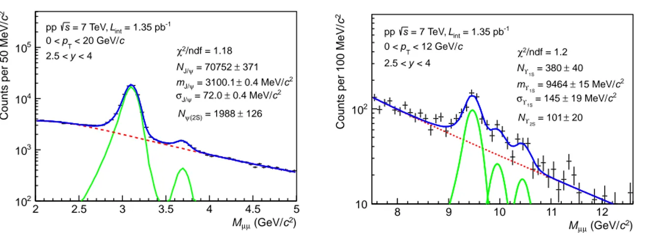
The normalization factors of the signal functions are left free, together with the position and the width of the J/ψsignal. On the other hand, the position and the width of theψ(2S) are tied to the corresponding parameters of the J/ψby forcing the mass difference between the two states to be equal to the one given by the Particle Data Group [39] and the mass resolution ratio to match the value obtained from a Monte Carlo (MC) simulation. The tail parameters for the J/ψ are determined by fitting the shape of the J/ψ signal obtained from the simulation. The same tail parameters are used for theψ(2S) as the resonances are separated by only 590 MeV/c2so that the energy straggling and multiple Coulomb scattering effects of the front absorber on the decay muons are expected to be similar. All the parameters of the functions used to fit the background are left free. An example of fit to the dimuon invariant mass distribution in the J/ψ andψ(2S) mass region is shown in the left panel of Fig. 1.
Theϒ(1S), (2S) and (3S) signal extractions are performed as for the J/ψandψ(2S) by fitting the dimuon invariant mass distribution in the mass range 5< mµµ < 15 GeV/c2. Due to the limited statistics, only theϒ(1S) andϒ(2S) yields are measured in this analysis. The background is fitted with a sum of either two power law or two exponential functions with all parameters left free. Each of the threeϒsignals (1S, 2S and 3S) is fitted with a Gaussian or a CB2 function. The fit parameters of theϒ(1S) signal are left free, whereas the width and mass position of theϒ(2S) andϒ(3S) are fixed with respect to the ones of the
ϒ(1S) in the same way as theψ(2S) parameters are fixed to the J/ψ. For the CB2 fit, the tail parameters of the function are fixed using the same method as for the charmonium signal extraction. An example of fit to the dimuon invariant mass distribution in theϒ’s mass region is shown in the right panel of Fig. 1.
2The Crystal Ball function consists of a Gaussian core and a power law tail at low masses, as defined in [40]. The CB2
) 2 c (GeV/ µ µ M 2 2.5 3 3.5 4 4.5 5 2 c
Counts per 50 MeV/
2 10 3 10 4 10 5 10 χ2/ndf = 1.18 -1 = 1.35 pb int L = 7 TeV, s pp c < 20 GeV/ T p 0 < < 4 y 2.5 < 371 ± = 70752 ψ J/ N 2 c 0.4 MeV/ ± = 3100.1 ψ J/ m 2 c 0.4 MeV/ ± = 72.0 ψ J/ σ 126 ± = 1988 (2S) ψ N ) 2 c (GeV/ µ µ M 8 9 10 11 12 2 c
Counts per 100 MeV/
10 2 10 -1 = 1.35 pb int L = 7 TeV, s pp c < 12 GeV/ T p 0 < < 4 y 2.5 < /ndf = 1.2 2 χ 40 ± = 380 1S ϒ N 2 c 15 MeV/ ± = 9464 1S ϒ m 2 c 19 MeV/ ± = 145 1S ϒ σ 20 ± = 101 2S ϒ N
Fig. 1: Dimuon invariant mass distribution in the region of charmonia (left) and bottomonia (right). Solid (dotted) lines correspond to signal (background) fit functions. The sum of the various fit functions is also shown as a solid line. For the J/ψ andψ(2S), a combination of two extended Crystal Ball functions is used for the signal and a variable width Gaussian function is used for the background. For theϒ resonances, a combination of extended Crystal Ball functions is used for the signals and two power law functions for the background.
About 70800 J/ψ, 2000ψ(2S), 380ϒ(1S) and 100ϒ(2S) have been measured with signal-to-background ratios (S/B), evaluated within three standard deviations with respect to the quarkonium pole mass, of 4, 0.2, 1 and 0.3, respectively.
In order to determine the pTdifferential cross sections, the data sample is divided in thirteen, nine and five transverse momentum intervals for J/ψ,ψ(2S) andϒ(1S), respectively. The differential cross section as a function of rapidity is evaluated in six intervals for the J/ψ andψ(2S) and three for theϒ(1S). Given the available statistics, only the measurement of the pT- and y-integratedϒ(2S) cross section is possible. The quarkonium raw yields obtained from the differential study are reported in Section 7. For J/ψ, the S/B ratio increases from 2.2 to 8.5 with increasing pT and from 3.7 to 5.4 with increasing rapidity. For
ψ(2S), it increases from 0.1 to 0.6 with increasing pTand from 0.1 to 0.2 with increasing rapidity. For theϒ(1S), no variation of the S/B ratio is observed within statistical uncertainties.
3.2 Acceptance and efficiency corrections
The measured yields obtained from the fits to the dimuon invariant mass distributions are corrected by the acceptance times efficiency factorhAεi to determine the production yields of the four resonances. In order to evaluate thehAεi factor, simulations of quarkonium production in pp collisions at√s= 7 TeV are performed with realistic pTand y distributions, obtained by fitting existing data measured at the same energy for J/ψandψ(2S) [42, 43], and by scaling CDF data [27] to√s= 7 TeV for theϒ. All resonances are forced to decay into two muons. Particle transport is performed using GEANT3 [44] and a realistic detector response is applied to the simulated hits in order to reproduce the performance of the apparatus during data taking. The same analysis cuts as used for the data are applied to the tracks reconstructed from these hits.
The simulations (one for each resonance) are performed on a run-by-run basis, using a realistic descrip-tion of the ALICE muon spectrometer performance. The misalignment of the muon spectrometer is tuned to reproduce the mass resolution of the J/ψ measured from data. The resonances are generated in a y range that is wider than the range used for the measurements (2.5 < y < 4) in order to account for edge effects. In each y and pT interval, the hAεi factor is calculated as the ratio of the number of reconstructed quarkonia over the number of quarkonia generated in this interval.
0.02)% forψ(2S), (20.93 ± 0.05)% for ϒ(1S) and(21.02 ± 0.05)% forϒ(2S), where the uncertainties are statistical. The hAεi correction factors associated to the pT and y differential yields are given in Section 7.
3.3 Systematic uncertainties
The main sources of systematic uncertainties on the production cross section come from the estimation of the number of measured quarkonia, the acceptance times efficiency correction factor and the integrated luminosity. The uncertainty on the dimuon branching ratio is also taken into account.
The systematic uncertainty on the signal extraction is evaluated using the Root Mean Square (RMS) of the results obtained with different signal functions (CB2 or pseudo-Gaussian functions for charmonia, CB2 or Gaussian functions for bottomonia), different background functions (VWG or Pol4×Exp for charmonia, the sum of two exponential or two power law functions for bottomonia) and different fitting ranges (beside the nominal fitting ranges quoted in Section 3.1 the ranges 2.5 < mµµ< 4.5 GeV/c2 and 8< mµµ< 12 GeV/c2were also used for charmonia and bottomonia, respectively). The tail parameters of the signal functions are also varied within the limits determined by fits to the simulated quarkonium mass distributions in the pT or y intervals used in the analysis. Finally, for the quarkonia analysis, different values for the ratio between the ψ(2S) and the J/ψ mass resolution have also been tested, estimated using a fit to the pT- and y-integrated invariant mass distribution with these parameters left free. The resulting systematic uncertainties averaged over pTand y are 2% for the J/ψ, 8% for theψ(2S), 8% for theϒ(1S) and 9% for theϒ(2S).
The systematic uncertainty on the acceptance times efficiency correction factor has several contributions: the parametrization of the input pTand y distributions of the simulated quarkonia, the track reconstruc-tion efficiency, the trigger efficiency and the matching between tracks in the muon tracking and triggering chambers. The acceptance times efficiency correction factors are evaluated assuming that all quarkonium states are unpolarized. If theϒ(1S) production polarization is fully transverse or fully longitudinal, then the cross section changes by about 37% and 20%, respectively. This result is consistent with previous studies made for charmonia [29, 30]. There is to date no evidence for a significant quarkonium polar-ization at √s= 7 TeV, neither for J/ψ [23], ψ(2S) [24, 25], nor for ϒ[26]. Therefore, no systematic uncertainty due to the quarkonium polarization has been taken into account.
For J/ψ and ψ(2S), the parametrization of the input pT and y distributions is based on fits to existing data measured at the same energy and in the same rapidity range [42, 43]. The corresponding systematic uncertainty is obtained by varying these parametrizations within the statistical and systematic uncertain-ties of the data, and taking the RMS of the resultinghAεi distribution. Correlations between pT and y observed by the LHCb collaboration [43] are also accounted for by evaluating thehAεi factors for each
pT (y) distribution measured in smaller y (pT) intervals and using the largest difference between the re-sulting values as an additional systematic uncertainty, quadratically summed to the one obtained using the procedure described above. For theϒ, simulations are based on pT and y parametrizations scaled from data measured by CDF [27] to√s= 7 TeV. The corresponding systematic uncertainty is evaluated by changing the energy of the scaled CDF data to √s= 4 TeV and √s= 10 TeV and evaluating the correspondinghAεi. This corresponds to a variation of the input yields of at most 15% as a function of rapidity and 40% as a function of pT. We note that extrapolating results obtained at a different collision energy is a conservative approach with respect to using CMS [45, 46] and LHCb [28] data at√s= 7 TeV. The resulting uncertainties are 1.7% for J/ψ andψ(2S), and 2.4% forϒ(1S) andϒ(2S).
The single muon tracking efficiency can be evaluated both in data [29] and in simulations. A difference of about 1.6% is observed which varies as a function of the muon pseudo-rapidity and pT. The impact of this difference onhAεi is quantified by replacing the single muon tracking efficiencies obtained from the simulated detector response with the values measured in the data. An additional uncertainty arising from the correlated inefficiency in the tracking chambers was evaluated and amounts to 2.5% at the dimuon
level. The resulting uncertainty on the corrected quarkonium yields amounts to 6.5% for all resonances. Concerning the trigger efficiency, a small difference is observed between data and simulations for the trigger response function. To account for this difference, a procedure similar to the one used for the systematic uncertainty on the track reconstruction efficiency is applied. The effect on hAεi amounts up to 2% for all resonances. Additional uncertainties come from the method used to determine the RPC efficiency from data (2%) and from the efficiency of the MB trigger condition for events where a quarkonium is produced (2%). The latter uncertainty is evaluated by means of a sample of events collected with a stand-alone dimuon trigger (without MB condition): the difference between the number of quarkonia reconstructed in such sample with and without the offline requirement of the MB condition is retained as uncertainty.
The difference observed in the simulations for different χ2 cuts on the matching between the tracks re-constructed in the tracking chambers and those rere-constructed in the trigger chambers leads to a systematic uncertainty of 1% onhAεi, independent from pTand y.
Finally, the uncertainty on the integrated luminosity amounts to 5%. It includes contributions from the MB trigger cross section (3.5% [38]), the MB trigger purity (3%, evaluated by varying the cuts defining the beam-beam and beam-gas collisions), possible effects on the MB trigger cross section from V0 aging between the moment when the vdM scan was performed and the data taking period (1.5%), the effects of V0 after-pulses and other instrumental effects on the MB trigger counts (1.5%, evaluated from fluctuations in the ratio of the MB trigger rate to a reference trigger rate provided by the T0).
A summary of the different systematic sources is given in Table 1 and the systematic uncertainties as-sociated to the pT and y differential cross sections are listed in Section 7. Concerning the pT and y dependence of these systematic uncertainties, the uncertainty associated to the luminosity is considered a global scale uncertainty, as is the uncertainty of the quarkonia branching ratio to dimuons. The one associated to the input MC parametrization is considered as largely point-to-point correlated. All other sources are considered as predominently uncorrelated.
Source J/ψ ψ(2S) ϒ(1S) ϒ(2S) Luminosity 5% 5% 5% 5% Signal extraction 2% (2%-15%) 8% (7.5%-11%) 8% (8%-13%) 9% Input MC parametrization 1.7% (0.1%-1.8%) 1.7% (0.4%-2.4%) 2.4% (0.6%-4.5%) 2.4% Trigger efficiency 3.5% (3%-5%) 3.5% (3%-5%) 3% 3% Tracking efficiency 6.5% (4.5%-11.5%) 6.5% (4.5%-11.5%) 6.5% (5.1%-10.5%) 6.5% Tracking-trigger matching 1% 1% 1% 1%
Table 1: Relative systematic uncertainties on the quantities associated to quarkonium cross section measurement. Into brackets, values correspond to the minimum and the maximum as a function of pTand y.
4 Results
4.1 Integrated and differential production cross sections of J/ψ andψ(2S)
The measured inclusive J/ψ andψ(2S) production cross sections in pp collisions at√s= 7 TeV in the rapidity range 2.5 < y < 4 are:
σJ/ψ= 6.69 ± 0.04(stat) ± 0.63(syst)µb, for 0< pT< 20 GeV/c,
σψ(2S)= 1.13 ± 0.07(stat) ± 0.19(syst)µb, for 0< pT< 12 GeV/c.
The measured J/ψ production cross section is in good agreement with the previously published ALICE result [29, 30].
) c (GeV/ T p 0 2 4 6 8 10 12 14 16 18 20 )) c b/(GeV/ µ ) ( y d T p /(d σ 2 d -5 10 -4 10 -3 10 -2 10 -1 10 1 pp s = 7 TeV, inclusive J/ψ, 2.5<y<4 5% ± -1 = 1.35 pb int L ALICE, 5.5% ± -1 = 15.6 nb int L ALICE, 10% ± -1 = 5.2 pb int L LHCb, Systematic uncertainty BR syst. unc. not shown
y -5 -4 -3 -2 -1 0 1 2 3 4 5 b) µ ( y /d σ d 0 2 4 6 8 10 12 ψ = 7 TeV, inclusive J/ s pp 5% ± -1 = 1.35 pb int L , -µ + µ ALICE 5.5% ± -1 = 15.6 nb int L , -µ + µ ALICE 4% ± -1 = 5.6 nb int L , -e + ALICE e 10% ± -1 = 5.2 pb int L LHCb, Systematic uncertainty BR syst. unc. not shown
) c (GeV/ T p 0 2 4 6 8 10 12 14 16 )) c b/(GeV/ µ ) ( y d T p /(d σ 2 d -4 10 -3 10 -2 10 -1 10 1 (2S) ψ = 7 TeV, inclusive s pp 5% ± -1 = 1.35 pb int L <4, y ALICE, 2.5< 1.3% ± -1 = 36 pb int L <4.5, y LHCb, 2< Systematic uncertainty BR syst. unc. not shown
y -5 -4 -3 -2 -1 0 1 2 3 4 5 b) µ ( y /d σ d 0 0.2 0.4 0.6 0.8 1 1.2 1.4 1.6 (2S) ψ = 7 TeV, inclusive s pp 5% ± -1 = 1.35 pb int L ALICE, Systematic uncertainty BR syst. unc. not shown
Fig. 2: Differential production cross sections of J/ψ (top) andψ(2S) (bottom) as a function of pT(left) and y
(right). The results are compared to previous ALICE results [29, 30] and LHCb measurements [42, 43]. The open symbols are the reflection of the positive-y measurements with respect to y= 0. The vertical error bars and the boxes represent the statistical and systematic uncertainties, respectively.
Figure 2 shows the differential production cross sections of J/ψ (top) andψ(2S) (bottom) as a function of pT(left) and rapidity (right). In all figures, the error bars represent the statistical uncertainties whereas the boxes correspond to the systematic uncertainties. The systematic uncertainty on the luminosity is quoted in the legend. This analysis extends the pT range of the J/ψ measurement with respect to the previous ALICE measurement [29, 30] from 8 GeV/c to 20 GeV/c.
The pTdifferential cross sections are compared with the values reported by the LHCb collaboration [42, 43]. The LHCb data points in Figure 2 correspond to the sum of prompt and b-meson decays quarkonium productions. For the J/ψ cross sections (Fig. 2, top left), a good agreement is observed between the two experiments. The comparison to the LHCb results for the pTdependence ofψ(2S) cross section (Fig. 2, bottom left) is not straightforward due to the different rapidity ranges. The ALICE measurement tends to be slightly higher than the one reported by LHCb, except at very low pT. Still, the results are in agreement within systematic uncertainties.
The differential cross sections of J/ψ as a function of rapidity (Fig. 2, top right) are compared to the previous measurements reported by ALICE [29, 30] and LHCb [42]. The results are in good agreement. Furthermore, the ALICE J/ψ measurement at mid-rapidity in the di-electron channel complements the forward rapidity measurement and allows to present the J/ψ differential cross section over a broad rapid-ity range for pTdown to zero. The rapidity dependence of the inclusiveψ(2S) production cross section at forward rapidity (Fig. 2, bottom right) is measured for the first time at√s= 7 TeV.
0.170 ± 0.011(stat.) ± 0.013(syst). To obtain this ratio, the same fit function (CB2 or pseudo-Gaussian function) is used for both resonances, for all the cases described in Section 3.3. The mean of the resulting distribution is used as the central value and its RMS is used as the systematic uncertainty on signal extraction. The other sources of systematic uncertainty cancel out in the ratio, except for the uncertainty on the hAεi factors. As a consequence of the adopted procedure, some differences between this value and the ratio of the integrated cross sections are expected.
) c (GeV/ T p 0 2 4 6 8 10 12 ) y d T p /(d ψ J/ σ 2 d ) y d T p /(d (2S) ψ σ 2 d 0 0.1 0.2 0.3 0.4 0.5 0.6 0.7 = 7 TeV s pp <4 y (2S), 2.5< ψ , ψ ALICE, inclusive J/ -1 = 1.35 pb int L <4.5 y (2S), 2< ψ , ψ LHCb, prompt J/ -1 (2S)) = 36 pb ψ ( int L , -1 ) = 5.2 pb ψ (J/ int L Systematic uncertainty BR syst. unc. not shown
y 2.6 2.8 3 3.2 3.4 3.6 3.8 4 y /d ψ J/ σ d y /d (2S) ψ σ d 0 0.05 0.1 0.15 0.2 0.25 0.3 0.35 = 7 TeV s pp -1 = 1.35 pb int L (2S), ψ , ψ ALICE, inclusive J/ Systematic uncertainty BR syst. unc. not shown
Fig. 3: ψ(2S)/J/ψ ratio as a function of pT (left) compared to LHCb measurement [43] and as a function of
rapidity (right).
Figure 3 presents the ψ(2S)-to-J/ψ cross section ratio as a function of pT (left) and y (right). This ratio increases with pT, whereas it shows little or no dependence on rapidity. The comparison with the LHCb measurement (left) shows a reasonable agreement, even though this analysis presents the ratio between inclusive cross sections whereas the LHCb collaboration reports the ratio between prompt particle cross sections, thus removing the contribution from b-meson decays. Assuming that theψ (2S)-to-J/ψ cross section ratio is independent of y over the entire rapidity range, as confirmed by ALICE measurements, and multiplying it by the branching ratio of ψ(2S) decaying into J/ψ plus anything
BRψ(2S)→J/ψ = 60.3 ± 0.7% [39], one gets the fraction of inclusive J/ψ coming from ψ(2S) decay
fψ(2S)= 0.103 ± 0.007(stat) ± 0.008(syst).
4.2 Integrated and differential production cross sections ofϒ(1S) andϒ(2S)
The measured inclusive ϒ(1S) and ϒ(2S) production cross sections, integrated over 2.5 < y < 4 and 0< pT< 12 GeV/c, are:
σϒ(1S)= 54.2 ± 5.0(stat) ± 6.7(syst) nb
σϒ(2S)= 18.4 ± 3.7(stat) ± 2.9(syst) nb.
The total number ofϒ(1S) extracted from the data allows to measure its differential production cross section in five pT intervals and three rapidity intervals. For theϒ(2S), on the contrary, no differential analysis could be performed due to the limited number of events.
Figure 4 presents theϒ(1S) differential production cross section as a function of pT (left) and the dif-ferential cross sections ofϒ(1S) and ϒ(2S) as a function of rapidity (right). Theϒ(1S) pT differential cross sections are compared to the values reported by the LHCb collaboration [28] in the same rapidity range (2.5 < y < 4). The results are in good agreement. Theϒ(1S) andϒ(2S) differential cross sections as a function of rapidity (Fig. 4 right) are presented together with the LHCb [28] and CMS [45, 46] measurements for pT down to zero. The measurements from ALICE and LHCb are in good agreement for bothϒstates.
) c (GeV/ T p 0 2 4 6 8 10 12 14 )) c ) (nb/(GeV/ y d T p /(d σ 2 d 1 10 pp s = 7 TeV, inclusive ϒ(1S), 2.5<y<4 5% ± -1 = 1.35 pb int L ALICE, 3.5% ± -1 = 25 pb int L LHCb, Systematic uncertainty BR syst. unc. not shown
y -5 -4 -3 -2 -1 0 1 2 3 4 5 (nb) y /d σ d 0 20 40 60 80 100 120 140 5% ± -1 = 1.35 pb int L (1S) ALICE, ϒ 3.5% ± -1 = 25 pb int L (1S) LHCb, ϒ 4% ± -1 = 36 pb int L (1S) CMS, ϒ = 7 TeV s pp (2S) ALICE ϒ (2S) LHCb ϒ (2S) CMS ϒ Systematic uncertainty
BR syst. unc. not shown
Fig. 4: Differential cross section ofϒ(1S) as a function of pT(left) and differential cross sections ofϒ(1S) and ϒ(2S) as function of rapidity (right), measured by ALICE, LHCb [28] and CMS [45, 46]. The open symbols are reflected with respect to y= 0.
The ϒ(2S)-to-ϒ(1S) cross section ratio at √s= 7 TeV integrated over pT and y is: σϒ(2S)/σϒ(1S) =
0.34 ± 0.10(stat) ± 0.02(syst). This ratio is in agreement with the one measured by the LHCb ex-periment [28]. Using a branching ratio for ϒ(2S) decaying intoϒ(1S) plus anything BRϒ(2S)→ϒ(1S) =
26.5 ± 0.5% [39], one gets the fraction of inclusiveϒ(1S) coming from ϒ(2S) decay fϒ(2S)= 0.090 ± 0.027(stat) ± 0.005(syst).
5 Model comparison
5.1 Differential production cross sections as a function of pT
The measured inclusive J/ψ differential production cross section as a function of pT is compared to three theoretical calculations performed in the CSM (Fig. 5): two complete calculations at LO and NLO respectively and a third calculation, called NNLO*, that includes the leading-pT contributions appearing at NNLO [47]. In agreement with the authors, the calculations are scaled by a factor 1/0.6 to account for the fact that they correspond to direct J/ψ production, whereas they are compared to inclusive measure-ments. This scaling factor is obtained by assuming that about 20% of the inclusive J/ψ come fromχc
decay [48], 10% fromψ(2S) (factor fψ(2S), Section 4) and 9% from b-mesons [42]. The LO calculation underestimates the data for pT > 2 GeV/c and the pT dependence is much steeper than the measured one. At NLO, the pT dependence is closer to that of the data, but the calculation still underestimates the measured cross section. The addition of some NNLO contributions further improves the agreement between data and theory concerning the pT dependence and further reduces the difference between the two, at the price of larger theoretical uncertainties.
Using a constant scaling factor for the direct-to-inclusive J/ψ production cross section ratio requires that the pT distributions of direct and decay J/ψ have the same shape. This assumption is a rather crude approximation and for instance the LHCb collaboration has measured a significant increase of the fraction of J/ψ from b-meson decay with pT up to 30% for pT> 14 GeV/c [42]. Properly accounting for these variations would improve the agreement between data and theory at large pT.
Figure 6 presents the comparison of the inclusive J/ψ differential production cross section (top), the inclusiveψ(2S) differential production cross section (middle) and the ratio between the two (bottom) as a function of pT to two NRQCD calculations for prompt J/ψ andψ(2S) production at NLO from [49] (left) and [19] (right). As discussed with the authors, a number of theoretical uncertainties cancels out when forming theψ(2S)-to-J/ψ ratio and the theory bands shown in the bottom panels are obtained by taking the ratio of theψ(2S) and J/ψ upper and lower bounds from top and middle panels separately,
) c (GeV/ T p 0 2 4 6 8 10 12 14 16 18 20 )) c b/(GeV/ µ ) ( y d T p /(d σ 2 d -5 10 -4 10 -3 10 -2 10 -1 10 1 10 2 10 Scaled CSM direct J/ψ LO NLO NNLO* <4 y , 2.5< ψ / J ALICE, inclusive Systematic uncertainty BR syst. unc. not shown
= 7 TeV s pp 5% ± -1 = 1.35 pb int L
Fig. 5: (color online). Inclusive J/ψdifferential production cross section as a function of pT, compared to several
scaled CSM calculations for direct J/ψ[47]. Details on the calculations are given in the text. rather than forming all four combinations.
The NRQCD calculations include both the same leading order Color-Singlet (CS) contributions as the one shown in Fig. 5 and Color-Octet (CO) contributions that are adjusted to experimental data by means of so-called Long-Range Matrix Elements (LRME). The two calculations differ in the LRME parametrization: the first (left panels of Fig. 6) uses three matrix elements whereas the second (right panels of Fig. 6) uses only two linear combinations of these three elements. Other differences include: the data sets used to fit these matrix elements, the minimum pT above which the calculation is appli-cable and the way by which contributions from χc decays into prompt J/ψ and ψ(2S) productions are
accounted for. The first calculation has significantly larger uncertainties than the second for both the J/ψ cross section and theψ(2S)-to-J/ψ ratio. This is a consequence of the differences detailed above and in particular the fact that the fits start at a lower pTand include a larger number of data sets.
Both calculations show reasonable agreement with data for all three observables. As it is the case for the CSM calculations, properly accounting for the contribution from b-meson decays to both J/ψ andψ(2S) inclusive productions in either the data or the theory would further improve the agreement at high pT. In the CSM, the directψ(2S) to direct J/ψ ratio is a constant, independent of pT and rapidity. It corre-sponds to the square of the ratio between theψ(2S) and J/ψwave functions at the origin and amounts to about 0.6 [47]3. This value, scaled by the direct-to-inclusive J/ψ andψ(2S) ratios (0.6 for J/ψ, as dis-cussed above, and 0.85 forψ(2S) [43]), becomes 0.42. It is larger than the pT-integrated measurement quoted in Section 4 and matches the values measured for pT> 9 GeV/c.
Concerning the increase of the inclusiveψ(2S)-to-J/ψ cross section ratio as a function of pT observed in the data, a fraction originates from the contribution ofψ(2S) andχcdecays. Assuming that the direct
production of all charmonium states follows the same pT distribution, as it is the case in the CEM, the transverse momentum of J/ψ coming from the decay of the higher mass resonances must be smaller than the one of the parent particle. This results in an increase of the corresponding contribution to the inclusive cross section ratio as a function of pT. The pT dependence resulting from this effect on the inclusive ψ(2S)-to-J/ψ cross section ratio has been investigated using PYTHIA [51] for decaying the parent particle into a J/ψ. The result is normalized to our measured integrated ψ(2S)-to-J/ψ cross section ratio and compared to the data in Fig. 7. As expected, an increase of the ratio is observed with increasing pT but it is not sufficient to explain the trend observed in the data. This indicates that the increase observed in the data cannot be entirely explained with simple decay kinematics arguments and that other effects must be taken into account. A non-constant ratio can already be expected in the
) c (GeV/ T p 0 2 4 6 8 10 12 14 16 18 20 )) c b/(GeV/ µ ) ( y d T p /(d σ 2 d -5 10 -4 10 -3 10 -2 10 -1 10 1 10 2 10 Prompt J/ψ CS+CO@NLO ) et al. (M. Butenschoen <4 y , 2.5< ψ / J ALICE, inclusive Systematic uncertainty BR syst. unc. not shown
= 7 TeV s pp 5% ± -1 = 1.35 pb int L ) c (GeV/ T p 0 2 4 6 8 10 12 14 16 18 20 )) c b/(GeV/ µ ) ( y d T p /(d σ 2 d -5 10 -4 10 -3 10 -2 10 -1 10 1 10 2 10 Prompt J/ψ CS+CO@NLO ) et al. (Y. Q. Ma <4 y , 2.5< ψ / J ALICE, inclusive Systematic uncertainty BR syst. unc. not shown
= 7 TeV s pp 5% ± -1 = 1.35 pb int L ) c (GeV/ T p 0 2 4 6 8 10 12 )) c b/(GeV/ µ ) ( y d T p /(d σ 2 d -3 10 -2 10 -1 10 1 (2S) CS+CO@NLO ψ Prompt ) et al. (M. Butenschoen <4 y (2S), 2.5< ψ ALICE, inclusive Systematic uncertainty BR syst. unc. not shown
= 7 TeV s pp 5% ± -1 = 1.35 pb int L ) c (GeV/ T p 0 2 4 6 8 10 12 )) c b/(GeV/ µ ) ( y d T p /(d σ 2 d -3 10 -2 10 -1 10 1 (2S) CS+CO@NLO ψ Prompt ) et al. (Y. Q. Ma <4 y (2S), 2.5< ψ ALICE, inclusive Systematic uncertainty BR syst. unc. not shown
= 7 TeV s pp 5% ± -1 = 1.35 pb int L ) c (GeV/ T p 0 2 4 6 8 10 12 ) y d T p /(dψ / J σ 2 d ) y d T p /(d (2S) ψ σ 2 d 0 0.1 0.2 0.3 0.4 0.5 0.6 0.7 = 7 TeV s pp -1 = 1.35 pb int L (2S), CS+CO@NLO ψ , ψ / J Prompt ) et al. (M. Butenschoen <4 y (2S), 2.5< ψ , ψ / J ALICE, inclusive Systematic uncertainty BR syst. unc. not shown
) c (GeV/ T p 0 2 4 6 8 10 12 ) y d T p /(dψ / J σ 2 d ) y d T p /(d (2S) ψ σ 2 d 0 0.1 0.2 0.3 0.4 0.5 0.6 0.7 = 7 TeV s pp -1 = 1.35 pb int L (2S), CS+CO@NLO ψ , ψ / J Prompt ) et al. (Y. Q. Ma <4 y (2S), 2.5< ψ , ψ / J ALICE, inclusive Systematic uncertainty BR syst. unc. not shown
Fig. 6: Inclusive J/ψdifferential production cross section (top), inclusiveψ(2S) differential production cross sec-tion (middle) and inclusiveψ(2S)-to-J/ψratio (bottom) as a function of pTcompared to two NRQCD calculations
from [49] (left) and [19] (right).
simplest case of CSM, where different diagram contributions to S- and P- wave charmonia production are expected, resulting in different feed-down contributions to J/ψ and ψ(2S). On top of this Color-Octet contributions can also be added, as done in the NRQCD framework. The proper accounting of such contributions is sufficient to reproduce the trend observed in the data, as shown in Fig. 6, bottom panels.
In Fig. 8, the inclusive ϒ(1S) differential production cross section as a function of pT is compared to three CSM calculations [52] (left) and to NRQCD [19] (right).
) c (GeV/ T p 0 2 4 6 8 10 12 ) y d T p /(dψ / J σ 2 d ) y d T p /(d (2S) ψ σ 2 d 0 0.1 0.2 0.3 0.4 0.5 0.6 0.7 = 7 TeV s pp -1 = 1.35 pb int L PYTHIA decayer <4 y (2S), 2.5< ψ , ψ / J ALICE, inclusive Systematic uncertainty BR syst. unc. not shown
Fig. 7: Inclusiveψ(2S)-to-J/ψcross section ratio as a function of pTcompared to a simulation in which all direct
quarkonia are considered to have the same pTdistribution and only kinematic effects due to the decay of higher
mass resonances are taken into account, using PYTHIA [51].
) c (GeV/ T p 0 2 4 6 8 10 12 )) c ) (nb/(GeV/ y d T p /(d σ 2 d -1 10 1 10 = 7 TeV s pp 5% ± -1 = 1.35 pb int L <4, y 2.5< (1S) Υ Scaled CSM direct LO NLO NNLO* (1S) Υ ALICE, inclusive Systematic uncertainty BR syst. unc. not shown
) c (GeV/ T p 0 2 4 6 8 10 12 )) c ) (nb/(GeV/ y d T p /(d σ 2 d -1 10 1 10 (1S) CS+CO@NLO Υ Inclusive (1S) Υ ALICE, inclusive Systematic uncertainty BR syst. unc. not shown
= 7 TeV s pp 5% ± -1 = 1.35 pb int L <4, y 2.5<
Fig. 8: (color online). Differential inclusive production cross section ofϒ(1S) as a function of pTcompared to
three scaled CSM calculations of directϒ(1S) [52] (left) and a NRQCD calculation of inclusiveϒ(1S) [55, 56] (right).
The CSM calculations are the same as for the J/ψ: two complete calculations at LO and NLO re-spectively and a calculation, called NNLO*, that includes the leading-pT contributions appearing at NNLO [52]. They have been scaled by a factor 1/0.6 to account for the contributions ofϒ(2S) (9 %, factor fϒ(2S), Section 4),ϒ(3S) (∼ 1% [28]) andχb(χb(1P)∼ 20% [53] andχb(2P)∼ 10% [54])
decay-ing intoϒ(1S). The comparison between these calculations and the data shows qualitatively the same features as for the J/ψ case: the LO calculation underestimates the data for pT> 4 GeV/c and falls too rapidly with increasing pT. The pTdependence of the NLO calculation is closer to that of the data, but the calculation still underestimates the cross section over the full pTrange. A good agreement is achieved at NNLO, but over a limited pTrange and with large theoretical uncertainties.
The NRQCD calculation is performed by the same group as in Fig. 6 (right) for the J/ψandψ(2S) [19]. It includes all the feed-down contributions from ϒ(2S), ϒ(3S) and χb. In the limited pT range of our measurement, the theory overestimates the data. This disagreement becomes smaller for increasing pT as it is also the case for the LHCb data [28].
In the CSM, the directϒ(2S) to directϒ(1S) cross section ratio is a constant equal to 0.45 [52]. In order to compare this value to the measurement quoted in Section 4, it must be scaled by the direct-to-inclusive
ϒ(1S) andϒ(2S) ratios. For ϒ(1S), we use a scaling factor of 0.6, as discussed above. Forϒ(2S), we consider a 5% contribution from ϒ(3S) [28] and neglect the contribution from χb, which has not been
measured to date. We get an upper limit for theϒ(2S) direct-to-inclusive ratio of 0.95 and consequently a lower limit for the scaled directϒ(2S)-to-ϒ(1S) ratio of 0.28. This lower limit is in good agreement with the measurement. We note that the measurement is also in good agreement with a NRQCD calculation performed at LO, as described in [57].
5.2 Differential production cross sections as a function of rapidity
y 2 2.5 3 3.5 4 4.5 b) µ ( y /d σ d 5 10 15 20 25 CS@LO ψ / J Scaled direct ψ / J ALICE, inclusive Systematic uncertainty BR syst. unc. not shown
= 7 TeV s pp 5% ± -1 = 1.35 pb int L y 2 2.5 3 3.5 4 4.5 (nb) y /d σ d 0 20 40 60 80
100 Scaled direct ALICE, inclusive Υ(1S) CS@LOΥ(1S) Systematic uncertainty BR syst. unc. not shown
= 7 TeV s pp 5% ± -1 = 1.35 pb int L
Fig. 9: (color online). Differential inclusive production cross sections of J/ψ (left) andϒ(1S) (right) as a function of y compared to a CSM calculation at LO [52].
Since the LO CSM calculations described in the previous section extend down to zero pT they can be integrated over pT and evaluated as a function of the quarkonium rapidity. The result is compared to the measured inclusive differential cross sections of J/ψandϒ(1S) in Fig. 9. As for the pTdifferential cross sections, the calculations are scaled by the direct-to-inclusive ratios described in the previous section (1/0.6 for J/ψ andϒ(1S)). Extending the calculation down to zero pTresults in large theoretical uncer-tainties: a factor four to five between the lower and upper bounds. The magnitude of the calculations is in agreement with the measurements. It is also worth noting that these calculations have no free parameters.
6 Conclusion
In conclusion, the inclusive production cross sections of J/ψ,ψ(2S),ϒ(1S) andϒ(2S) as a function of
pTand y have been measured using the ALICE detector at forward rapidity (2.5 < y < 4) in pp collisions at a centre of mass energy√s= 7 TeV. For J/ψ, the measurements reported here represent an increase by a factor of about 80 in terms of luminosity with respect to published ALICE results, whereas they are the first ALICE measurements for the other three quarkonium states. The measured inclusive cross sections, integrated over pTand y are: σJ/ψ= 6.69 ± 0.04 ± 0.63 µb,σψ(2S)= 1.13 ± 0.07 ± 0.19µb,
σϒ(1S)= 54.2 ± 5.0 ± 6.7 nb and σϒ(2S)= 18.4 ± 3.7 ± 2.9 nb, where the first uncertainty is statistical
and the second one is systematic, assuming no quarkonium polarization. Measuring both J/ψ andψ(2S) cross sections with the same apparatus and the same data set allows deriving the fraction of inclusive J/ψ that comes from ψ(2S) decay with reduced systematic uncertainties: fψ(2S)= 0.103 ± 0.007 ± 0.008. Similarly, the fraction of inclusiveϒ(1S) that comes fromϒ(2S) decay is fϒ(2S)= 0.090 ±0.027±0.005. These results are in good agreement with measurements from the LHCb experiment over similar pT and y ranges. For ϒ(1S) and ϒ(2S) they complement the measurements from CMS at mid-rapidity (|y| < 2.4). They are also in good agreement with NRQCD calculations for which the matrix elements have been fitted to data sets from Tevatron, RHIC and LHC, among others. In the CSM, both LO and NLO calculations underestimate the data at large pT as it was the case at lower energy. The addition of
the leading-pT NNLO contributions helps to reduce this disagreement at the price of larger theoretical uncertainties. LO calculations reproduce qualitatively the data at low pTand the rapidity dependence of the pT-integrated cross sections.
7 Integrated and differential quarkonium yields and cross sections
In the following tables, the systematic uncertainties correspond to the quadratic sum of the different sources presented in Section 3.3 without the contribution from the luminosity and the branching ratios.
Aε corresponds to the acceptance times efficiency factor.
0< pT< 20 (GeV/c) N± stat Aε± stat (%) σ± stat ± syst 2.5 < y < 4
J/ψ 70752± 371 13.22 ± 0.02 6.69 ± 0.04 ± 0.53µb 0< pT< 12 (GeV/c) N± stat Aε± stat (%) σ± stat ± syst
2.5 < y < 4
ψ(2S) 1987± 127 16.64 ± 0.02 1.13 ± 0.07 ± 0.12µb
ϒ(1S) 380± 35 20.93 ± 0.05 54.23 ± 5.01 ± 5.98 nb
ϒ(2S) 101± 20 21.02 ± 0.05 18.44 ± 3.70 ± 2.18 nb
Table 2: Integrated raw yields and cross sections of J/ψ,ψ(2S),ϒ(1S) andϒ(2S) for pp collisions at√s= 7 TeV.
pT NJ/ψ± stat Aε± stat d2σJ/ψ/(d pTdy) ± stat ± syst
(GeV/c) (%) (µb/(GeV/c)) [0; 1] 10831± 161 12.51 ± 0.06 0.721 ± 0.011 ± 0.049 [1; 2] 17303± 196 10.67 ± 0.04 1.350 ± 0.015 ± 0.093 [2; 3] 13859± 162 10.92 ± 0.05 1.057 ± 0.012 ± 0.068 [3; 4] 10134± 133 13.49 ± 0.05 0.626 ± 0.008 ± 0.038 [4; 5] 7009± 103 17.20 ± 0.06 0.339 ± 0.005 ± 0.020 [5; 6] 4398± 81 21.32 ± 0.07 0.172 ± 0.003 ± 0.011 [6; 8] 4392± 80 26.53 ± 0.06 0.0689 ± 0.0013 ± 0.0044 [8; 10] 1569± 47 32.75 ± 0.06 0.0199 ± 0.0006 ± 0.0013 [10; 12] 628± 31 37.31 ± 0.07 0.0070 ± 0.0003 ± 0.0005 [12; 14] 287± 24 40.59 ± 0.08 0.0029 ± 0.0002 ± 0.0002 [14; 16] 128± 17 42.95 ± 0.08 0.0012 ± 0.0002 ± 0.0001 [16; 18] 65± 11 44.80 ± 0.10 0.0006 ± 0.0001 ± 0.0001 [18; 20] 33± 10 46.03 ± 0.11 0.0003 ± 0.0001 ± 0.0001 y NJ/ψ± stat Aε± stat (%) dσJ/ψ/dy ± stat ± syst (µb)
[2.5; 2.75] 4660± 93 4.07 ± 0.03 5.72 ± 0.11 ± 0.60 [2.75; 3.0] 14768± 165 13.97 ± 0.05 5.28 ± 0.06 ± 0.59 [3.0; 3.25] 18559± 196 19.97 ± 0.07 4.64 ± 0.05 ± 0.55 [3.25; 3.5] 17241± 185 20.35 ± 0.07 4.23 ± 0.05 ± 0.50 [3.5; 3.75] 11727± 148 15.30 ± 0.06 3.83 ± 0.05 ± 0.43 [3.75; 4.0] 3691± 82 5.49 ± 0.03 3.36 ± 0.08 ± 0.33
pT Nψ(2S)± stat Aε± stat d2σψ(2S))/(d pTdy) ± stat ± syst (GeV/c) (%) (µb/(GeV/c)) [0; 1] 191± 52 17.63 ± 0.07 0.069 ± 0.019 ± 0.008 [1; 2] 572± 73 15.51 ± 0.06 0.234 ± 0.030 ± 0.028 [2; 3] 350± 57 14.18 ± 0.05 0.156 ± 0.025 ± 0.017 [3; 4] 259± 42 14.87 ± 0.06 0.110 ± 0.018 ± 0.014 [4; 5] 197± 30 17.01 ± 0.06 0.073 ± 0.011 ± 0.0090 [5; 6] 150± 28 20.15 ± 0.07 0.047 ± 0.0088 ± 0.0059 [6; 8] 111± 24 24.81 ± 0.05 0.0142 ± 0.0031 ± 0.0014 [8; 10] 69± 15 30.75 ± 0.06 0.0071 ± 0.0015 ± 0.0007 [10; 12] 33± 11 35.28 ± 0.07 0.0030 ± 0.0010 ± 0.0004 y Nψ(2S)± stat Aε± stat (%) dσψ(2S)/dy ± stat ± syst (µb)
[2.5; 2.75] 117± 36 5.63 ± 0.03 0.79 ± 0.24 ± 0.11 [2.75; 3.0] 402± 58 18.10 ± 0.06 0.84 ± 0.12 ± 0.13 [3.0; 3.25] 538± 67 25.12 ± 0.07 0.81 ± 0.10 ± 0.12 [3.25; 3.5] 480± 63 25.20 ± 0.07 0.72 ± 0.10 ± 0.10 [3.5; 3.75] 344± 48 18.67 ± 0.06 0.70 ± 0.10 ± 0.10 [3.75; 4.0] 93± 26 6.58 ± 0.04 0.54 ± 0.15 ± 0.07
Table 4: Differential raw yields and cross sections ofψ(2S) for pp collisions at√s= 7 TeV.
pT (GeV/c) ( d2σψ(2S) d pTdy )/( d2σJ/ψ d pTdy) ± stat ± syst [0; 1] 0.097 ± 0.026 ± 0.007 [1; 2] 0.173 ± 0.022 ± 0.015 [2; 3] 0.148 ± 0.024 ± 0.011 [3; 4] 0.176 ± 0.029 ± 0.019 [4; 5] 0.215 ± 0.033 ± 0.019 [5; 6] 0.282 ± 0.050 ± 0.028 [6; 8] 0.218 ± 0.045 ± 0.016 [8; 10] 0.356 ± 0.078 ± 0.028 [10; 12] 0.42 ± 0.14 ± 0.03 y (dσψ(2S) dy )/( dσJ/ψ dy ) ± stat ± syst [2.5; 2.75] 0.137 ± 0.042 ± 0.013 [2.75; 3.0] 0.160 ± 0.024 ± 0.016 [3.0; 3.25] 0.175 ± 0.022 ± 0.014 [3.25; 3.5] 0.171 ± 0.023 ± 0.013 [3.5; 3.75] 0.183 ± 0.026 ± 0.017 [3.75; 4.0] 0.160 ± 0.046 ± 0.017
pT Nϒ(1S)± stat Aε± stat d2σϒ(1S)/(d pTdy) ± stat ± syst (GeV/c) (%) (nb/(GeV/c)) [0; 2] 59± 13 20.21 ± 0.18 2.91 ± 0.64 ± 0.31 [2; 4] 126± 19 20.04 ± 0.13 6.26 ± 0.94 ± 0.64 [4; 6] 86± 21 20.13 ± 0.13 4.25 ± 1.04 ± 0.53 [6; 8] 47± 13 20.38 ± 0.16 2.30 ± 0.64 ± 0.27 [8; 12] 47± 13 21.76 ± 0.17 1.08 ± 0.30 ± 0.14
y Nϒ(1S)± stat Aε± stat (%) dσϒ(1S)/dy ± stat ± syst (nb)
[2.5; 3] 121± 19 15.47 ± 0.10 46.7 ± 7.4 ± 6.1 [3; 3.5] 200± 30 31.34 ± 0.13 38.1 ± 5.8 ± 6.6 [3.5; 4.0] 67± 14 16.32 ± 0.12 24.5 ± 5.0 ± 3.3
Acknowledgements
We are grateful to M. Butenschoen, K.-T. Chao, R.L. Kisslinger and J.-P. Lansberg for providing us model calculations and for intensive discussions.
The ALICE Collaboration would like to thank all its engineers and technicians for their invaluable contributions to the construction of the experiment and the CERN accelerator teams for the outstanding performance of the LHC complex.
The ALICE Collaboration gratefully acknowledges the resources and support provided by all Grid centres and the Worldwide LHC Computing Grid (WLCG) collaboration.
The ALICE Collaboration acknowledges the following funding agencies for their support in building and running the ALICE detector:
State Committee of Science, World Federation of Scientists (WFS) and Swiss Fonds Kidagan, Armenia, Conselho Nacional de Desenvolvimento Científico e Tecnológico (CNPq), Financiadora de Estudos e Projetos (FINEP), Fundação de Amparo à Pesquisa do Estado de São Paulo (FAPESP);
National Natural Science Foundation of China (NSFC), the Chinese Ministry of Education (CMOE) and the Ministry of Science and Technology of China (MSTC);
Ministry of Education and Youth of the Czech Republic;
Danish Natural Science Research Council, the Carlsberg Foundation and the Danish National Research Foundation;
The European Research Council under the European Community’s Seventh Framework Programme; Helsinki Institute of Physics and the Academy of Finland;
French CNRS-IN2P3, the ‘Region Pays de Loire’, ‘Region Alsace’, ‘Region Auvergne’ and CEA, France;
German BMBF and the Helmholtz Association;
General Secretariat for Research and Technology, Ministry of Development, Greece; Hungarian OTKA and National Office for Research and Technology (NKTH);
Department of Atomic Energy and Department of Science and Technology of the Government of India; Istituto Nazionale di Fisica Nucleare (INFN) and Centro Fermi - Museo Storico della Fisica e Centro Studi e Ricerche "Enrico Fermi", Italy;
MEXT Grant-in-Aid for Specially Promoted Research, Japan; Joint Institute for Nuclear Research, Dubna;
National Research Foundation of Korea (NRF);
CONACYT, DGAPA, México, ALFA-EC and the EPLANET Program (European Particle Physics Latin American Network)
Stichting voor Fundamenteel Onderzoek der Materie (FOM) and the Nederlandse Organisatie voor Wetenschappelijk Onderzoek (NWO), Netherlands;
Research Council of Norway (NFR);
Polish Ministry of Science and Higher Education; National Science Centre, Poland;
Ministry of National Education/Institute for Atomic Physics and CNCS-UEFISCDI - Romania; Ministry of Education and Science of Russian Federation, Russian Academy of Sciences, Russian Federal Agency of Atomic Energy, Russian Federal Agency for Science and Innovations and The Russian Foundation for Basic Research;
Ministry of Education of Slovakia;
Department of Science and Technology, South Africa;
CIEMAT, EELA, Ministerio de Economía y Competitividad (MINECO) of Spain, Xunta de Galicia (Consellería de Educación), CEADEN, Cubaenergía, Cuba, and IAEA (International Atomic Energy Agency);
Swedish Research Council (VR) and Knut & Alice Wallenberg Foundation (KAW); Ukraine Ministry of Education and Science;
United Kingdom Science and Technology Facilities Council (STFC);
The United States Department of Energy, the United States National Science Foundation, the State of Texas, and the State of Ohio.
References
[1] M. Cacciari, M. Greco, and P. Nason, J. High Energy Phys. 9805 (1998) 007, arXiv:9803400 [hep-ph].
[2] M. Cacciari, S. Frixione, and P. Nason, J. High Energy Phys. 0103 (2001) 006, arXiv:0102134 [hep-ph].
[3] M. Cacciari et al., J. High Energy Phys. 1210 (2012) 137,arXiv:1205.6344 [hep-ph]. [4] N. Brambilla et al., Eur. Phys. J. C 71 (2011) 1534,arXiv:1010.5827 [hep-ph]. [5] M.B. Einhorn and S.D. Ellis, Phys. Rev. D 12 (1975) 2007.
[6] C.E. Carlson and R. Suaya, Phys. Rev. D 14 (1976) 3115. [7] R. Baier and R. Rückl, Phys. Lett. B 102 no. 5, (1981) 364. [8] F. Abe et al. (CDF Collaboration), Phys. Rev. Lett. 79 (1997) 572.
[9] J. M. Campbell, F. Maltoni, and F. Tramontano, Phys. Rev. Lett. 98 (2007) 252002, arXiv:hep-ph/0703113 [HEP-PH].
[10] P. Artoisenet et al., Phys. Rev. Lett. 101 (2008) 152001,arXiv:0806.3282 [hep-ph]. [11] J.-P. Lansberg, Eur. Phys. J. C 61 (2009) 693,arXiv:0811.4005 [hep-ph].
[12] E. Braaten et al., Phys. Lett. B 333 (1994) 548,arXiv:9405407 [hep-ph]. [13] P. Artoisenet, J.-P. Lansberg, and F. Maltoni, Phys. Lett. B 653 (2007) 60,
arXiv:0703129 [hep-ph].
[14] H. Haberzettl and J. P. Lansberg, Phys. Rev. Lett. 100 (2008) 032006,arXiv:0709.3471 [hep-ph].
[15] F. Halzen, Phys. Lett. B 69 (1977) 105. [16] H. Fritzsch, Phys. Lett. B 67 (1977) 217.
[17] J. Amundson et al., Phys. Lett. B 390 (1997) 323,arXiv:9605295 [hep-ph]. [18] G. T. Bodwin, E. Braaten, and G. P. Lepage, Phys. Rev. D 51 (1995) 1125,
arXiv:9407339 [hep-ph].
[19] Y. Q. Ma, K. Wang, and K. T. Chao, Phys. Rev. D 84 (2011) 114001, arXiv:1012.1030 [hep-ph].
[20] M. Butenschoen and B. A. Kniehl, Phys. Rev. Lett. 106 (2011) 022003, arXiv:1009.5662 [hep-ph].
[21] G. Xu et al., Phys. Rev. D 86 (2012) 094017,arXiv:1203.0207 [hep-ph]. [22] A. Abulencia et al. (CDF Collaboration), Phys. Rev. Lett. 99 (2007) 132001,
arXiv:0704.0638 [hep-ex].
[23] B. Abelev et al. (ALICE Collaboration), Phys. Rev. Lett. 108 (2012) 082001, arXiv:1111.1630 [hep-ex].
[24] R. Aaij et al. (LHCb Collaboration), Eur. Phys. J. C 73 (2013) 2631, arXiv:1307.6379 [hep-ex].
[25] S. Chatrchyan et al. (CMS Collaboration),arXiv:1307.6070 [hep-ex]. [26] S. Chatrchyan et al. (CMS Collaboration), Phys. Rev. Lett. 110 (2013) 081802,
arXiv:1209.2922 [hep-ex].
[27] F. Abe et al. (CDF Collaboration), Phys. Rev. Lett. 75 (1995) 4358. [28] R. Aaij et al. (LHCb Collaboration), Eur. Phys. J. C 72 (2012) 2025,
arXiv:1202.6579 [hep-ex].
[29] K. Aamodt et al. (ALICE Collaboration), Phys. Lett. B 704 (2011) 442, arXiv:1105.0380 [hep-ex].
[30] K. Aamodt et al. (ALICE Collaboration), Phys. Lett. B 718 no. 2, (2012) 692. [31] K. Aamodt et al. (ALICE Collaboration), J. Instrum. 3 (2008) S08002. [32] K. Aamodt et al. (ALICE Collaboration), J. Instrum. 5 (2010) 3003,
arXiv:1001.0502 [physics.ins-det].
[33] E. Abbas et al. (ALICE Collaboration),arXiv:1306.3130 [nucl-ex]. [34] M. Bondila et al., IEEE Trans. Nucl. Sci. 52 (2005) 1705.
[35] F. Bossù, M. Gagliardi, and M. Marchisone (ALICE Collaboration), J. Instrum. 7 no. 12, (2012) T12002.
[36] R. Arnaldi et al., Nucl. Phys. Proc. Suppl. 158 (2006) 21–24. [37] S. van der Meer, ISR-PO/68-31, KEK68-64.
[38] B. Abelev et al. (ALICE Collaboration), Eur. Phys. J. C 73 (2013) 2456, arXiv:1208.4968 [hep-ex].
[39] J. Beringer et al. (Particle Data Group), Phys. Rev. D 86 (2012) 010001. [40] J. Gaiser et al., Phys. Rev. D 34 (1986) 711.
[41] R. Shahoyan, J/ψ andψ(2S) production in 450 GeV pA interactions and its dependence on the rapidity and xF. PhD thesis, 2001.
[42] R. Aaij et al. (LHCb Collaboration), Eur. Phys. J. C 71 (2011) 1645, arXiv:1103.0423 [hep-ex].
[43] R. Aaij et al. (LHCb Collaboration), Eur. Phys. J. C 72 (2012) 2100, arXiv:1204.1258 [hep-ex].
[44] R. Brun et al., CERN Program Library Long Write-up W5013 (1994) . [45] V. Khachatryan et al. (CMS Collaboration), Phys. Rev. D 83 (2011) 112004,
arXiv:1012.5545 [hep-ex].
[46] S. Chatrchyan et al. (CMS Collaboration), Phys. Lett. B 727 (2013) 101, arXiv:1303.5900 [hep-ex].
[47] J.-P. Lansberg, J. Phys. G 38 (2011) 124110,arXiv:1107.0292 [hep-ph].
[48] R. Aaij et al. (LHCb Collaboration), Phys. Lett. B 718 (2012) 431,arXiv:1204.1462 [hep-ex]. [49] M. Butenschoen and B. A. Kniehl, Phys. Rev. D 84 (2011) 051501,
arXiv:1105.0820 [hep-ph].
[50] E. J. Eichten and C. Quigg, Phys. Rev. D 52 (1995) 1726,arXiv:9503356 [hep-ph]. [51] T. Sjostrand, S. Mrenna, and P. Z. Skands, J. High Energy Phys. 0605 (2006) 026,
arXiv:hep-ph/0603175 [hep-ph].
[52] J.-P. Lansberg, Nucl. Phys. A 470 (2013) 910,arXiv:1209.0331 [hep-ph]. [53] R. Aaij et al. (LHCb Collaboration), J. High Energy Phys. 1211 (2012) 031,
arXiv:1209.0282 [hep-ex].
[54] T. Affolder et al. (CDF Collaboration), Phys. Rev. Lett. 84 (2000) 2094, arXiv:hep-ex/9910025 [hep-ex].
[55] K. Wang, Y. Q. Ma and K. T. Chao, Phys. Rev. D 85 (2012) 114003, arXiv:1202.6012 [hep-ph].
[56] K. Wang, Y. Q. Ma and K. T. Chao, private communication.
[57] L. S. Kisslinger and D. Das, Mod. Phys. Lett. A 28 (2013) 1350120, arXiv:1306.6616 [hep-ph].


![Fig. 4: Differential cross section of ϒ(1S) as a function of p T (left) and differential cross sections of ϒ(1S) and ϒ(2S) as function of rapidity (right), measured by ALICE, LHCb [28] and CMS [45, 46]](https://thumb-eu.123doks.com/thumbv2/123doknet/14073977.462799/11.892.123.789.125.365/differential-section-function-differential-sections-function-rapidity-measured.webp)
![Fig. 5: (color online). Inclusive J/ ψ differential production cross section as a function of p T , compared to several scaled CSM calculations for direct J/ ψ [47]](https://thumb-eu.123doks.com/thumbv2/123doknet/14073977.462799/12.892.280.616.121.367/online-inclusive-differential-production-section-function-compared-calculations.webp)
![Fig. 6: Inclusive J/ ψ differential production cross section (top), inclusive ψ (2S) differential production cross sec- sec-tion (middle) and inclusive ψ (2S)-to-J/ ψ ratio (bottom) as a function of p T compared to two NRQCD calculations from [49] (left) a](https://thumb-eu.123doks.com/thumbv2/123doknet/14073977.462799/13.892.114.815.119.870/inclusive-differential-production-inclusive-differential-production-inclusive-calculations.webp)


