HAL Id: hal-00307402
https://hal.archives-ouvertes.fr/hal-00307402
Submitted on 1 Dec 2008
HAL is a multi-disciplinary open access archive for the deposit and dissemination of sci-entific research documents, whether they are pub-lished or not. The documents may come from teaching and research institutions in France or abroad, or from public or private research centers.
L’archive ouverte pluridisciplinaire HAL, est destinée au dépôt et à la diffusion de documents scientifiques de niveau recherche, publiés ou non, émanant des établissements d’enseignement et de recherche français ou étrangers, des laboratoires publics ou privés.
Toward a quantification of self-similarity in plants
Pascal Ferraro, Christophe Godin, Przemylaw Prusinkiewicz
To cite this version:
Pascal Ferraro, Christophe Godin, Przemylaw Prusinkiewicz. Toward a quantification of self-similarity in plants. Fractals, World Scientific Publishing, 2005, 13, pp.91-109. �10.1142/S0218348X05002805�. �hal-00307402�
Toward a quantification of self-similarity in plants
Pascal Ferraro
∗Christophe Godin
†Przemyslaw Prusinkiewicz
‡Abstract
Self-similarity of plants has attracted the attention of biologists for at least 50 years, yet its formal treatment is rare, and no measure for quantifying the degree of self-similarity currently exists. We propose a formal definition and measures of self-similarity, tailored to branching plant structures. To evaluate self-similarity, we make use of an algorithm for computing topological distances between branching systems, developed in computer science. The formalism is illustrated using theoretical branching systems, and applied to analyze self-similarity in two sample plant structures: inflorescences of Syringa vulgaris (lilac) and shoots of Oryza sativa (rice).
Key words: Selfsimilarity fractal paracladial relationship branching structure -structural comparison - edit distance.
1
INTRODUCTION
Repetitive patterns are readily noticeable in the growth and structure of many living organisms. In particular, modular organization is an essential element of the development
∗LaBRI - University of Bordeaux 1, 351 Cours de la Lib´eration, 33405 Talence Cedex, France. E-mail:
†INRIA, UMR AMAP, TA40/PSII, Boulevard de la Lironde, 34398 Montpellier Cedex 5, France.
E-mail: [email protected]
‡Department of Computer Science, University of Calgary, Calgary, Alberta T2N 1N4, Canada. E-mail:
and structure of plants.1, 2, 3, 4, 5 This is essential to the understanding of plant biology,
and plays an important role in the formal analysis6 and simulation7, 8 of plants.
In some cases, the modules are arranged into compound, recursively nested, fractal-like structures, with similar patterns appearing at different scales9 (Fig. 1). In botany, an early study of such structures is due to Arber.10 Troll11 defined a compound
inflo-rescence as a system consisting of the main floinflo-rescence and paracladia (term introduced originally by Schultz12) that repeat the structure of the main florescence. This concept
was later formalized by Fritjers and Lindemayer,13 who defined paracladia as “branches
which repeat the florescence of the main axis and which on their turn can give rise to paracladia of their own.” Prusinkiewicz et al.14 introduced a related concept of branch
mapping, according to which, “given two branches of the same order, the shorter branch is identical [...] to the top portion of the longer branch.” M¨undermann15 further studied
these concepts as a basis for constructing three-dimensional plant models. More recently, Prusinkiewicz16 introduced the notion of topological self-similarity, which relates plant
self-similarity to the theory of L-systems.17, 18, 8
In comparison to inflorescences, self-similar organization is less obvious in trees, which develop over a longer period of time, and therefore are more prone to the influences of the environment. Nevertheless, the branching systems of trees also result from repetitive processes, in which various meristems follow similar sequences of states and produce similar structures as a result. These sequences have been characterized by biologists in such terms as age state,19 morphogenetic program,20 and physiological age.21 This
last notion made it possible, for example, to exploit similarities in the development and structure of Zelkova serrata (Japanese elm) in the construction of a simulation model,22
where the sequence of physiological ages of a typical meristem in the plant served as a template (called the reference axis) for all plant meristems.
Self-similarity, like symmetry, is not easily quantifiable: it is usually considered to be either absent or present. Real plants, however, may be self-similar only to some degree. In this paper, we propose a definition of self-similarity in branching structures, and describe
a procedure for quantifying it in measured or simulated plants. This procedure is based on a method for comparing tree-like structures introduced by Zhang23 and extended to
the problem of comparing plants.24, 25 We first analyze the self-similarity measures using
branching structures with controlled, algorithmically generated topology. We then apply these measures to analyze self-similarity in two real plant structures obtained from field measurements.
2
THEORETICAL CONCEPTS
2.1
Self-Similarity of Axial Trees
A plant is viewed as an assembly of adjacent botanical components such as internodes or annual growth increments.26 Such a structure can be formally described by defining
a set of vertices V that represent the plant components (each vertex corresponding to a plant part: internode, growth unit, etc.), and a list E of pairs of vertices that describes the adjacency of these components.6 We assume that each component v is physically
attached to the plant body through at most one parent component, denoted parent(v). The resulting topological structure is called a rooted tree graph T = (V, E). In such a graph, every vertex except one (the root r) has exactly one parent vertex: the root has no parent. In the following, a tree graph rooted in r will be denoted by T [r], and the empty tree graph will be denoted by θ = (∅, ∅). In order to identify the different axes on a given plant, two types of relations between entities are distinguished: an entity can either precede (symbol <) or bear (symbol +) another entity. An axial tree8 is then defined
as a rooted tree in which an entity can be attached to at most one other entity by a < connection. Formally, we have:
Definition 1 (Axial tree) An axial tree is a graph T = (V, E, α), where V is a finite vertex set, E is a finite set of ordered vertex pairs, and α is a mapping of E into {<,+}, provided that:
• T = (V, E) is a rooted tree, and
• the edge type function α satisfies the condition:
if α(x, y) = α(x, z) = ‘<’ then y = z
for all (x, y) ∈ E and (x, z) ∈ E.
We define the axis of v as the set of vertices that are connected to the given vertex v through paths consisting only of ‘<’-edges. The second property of Definition 1 implies that this axis is always a linear sequence of vertices. We denote this sequence by A(v):
A(v) = {v1, v2, ..., vn} if v1 = v and α(vi, vi+1) = ‘<’ for all i = 1, 2, · · · , n − 1. (1)
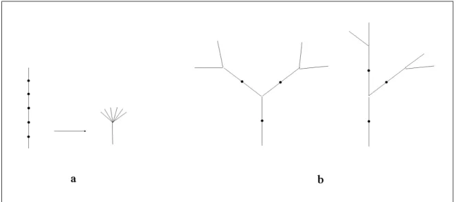
We call the axis A(r) of the root r of T the trunk of T . For any vertex v, rank(v) is the number of vertices in A(v). These definitions are illustrated in Figs. 2.a,b.
Definition 2 (Axial tree isomorphism) Let us consider two axial trees, T1 = (V1, E1, α1)
and T2 = (V2, E2, α2). A bijection φ from V1 to V2 is an axial tree isomorphism if:
• for each (x, y) ∈ E1, (φ(x), φ(y)) ∈ E2, and
• α2(φ(x), φ(y)) = α1(x, y).
Two structures T1 and T2 are thus isomorphic (denoted T1 ≡ T2) if they are identical
except for the labels of their components. We can now formalize the notion of paracladia:
Definition 3 (Paracladium) Let v be a vertex of T . T [v] is a paracladium of T if there exists a vertex w in the trunk of T such that T[v] ≡ T [w].
The notion of paracladium enables us to define a notion of self-similarity which cap-tures the main feacap-tures of nested struccap-tures discussed in the introduction.
Definition 4 (Self-similarity) An axial tree T is self-similar if all of its sub-branching systems are paracladia, i.e. ∀v ∈ V , T [v] is a paracladium of T .
In a self-similar axial tree, the trunk provides a template for the branching pattern of the entire structure. A small branching system is isomorphic to a distal part of the trunk branching system, while a large branching structure is isomorphic to a larger distal part of the trunk branching system. Figure 3 illustrates this definition using different self-similar branching structures as examples. We note that self-similar structures may have different degrees of apparent structural complexity, related to their maximum branching order.
Now, let us consider the question of deciding whether a given axial tree structure is self-similar. A naive approach based on Definition 4 would consist of checking, for each vertex v of the tree, whether there is a corresponding vertex w of the trunk such that T [v] ≡ T [w]. However, the following proposition enables us to greatly simplify this approach by making use of the recursive character of self-similar branching structures.
For any vertex v ∈ V, let us call B(v) the set of vertices x ∈ V , such that x 6∈ A(v) and parent(x) ∈ A(v). B(r), for example, is the set of root vertices of all first-order branches of the tree T [r] (Fig. 2.c).
Proposition 5 An axial tree T [r] is self-similar if and only if for every vertex v ∈ B(r), the branch T[v] is a paracladium of T [r].
The proof is given in the appendix. Its intuition is as follows. Suppose that all of the first-order branches have been proved to be paracladial. This means that any such branch B1 is isomorphic to some distal part T1 of the trunk (Figure 4.a and b). Any
second-order branch B2 of B1 is then isomorphic to a branch T2 of T1. However, a branch
of T1 is a first-order branch; hence, by hypothesis, T2 is a paracladium, and so must be
B2. By applying this argument recursively we show that any branch Bnis a paracladium,
because branch Bn of order n is isomorphic to some branch Bn−1 of order n − 1, which in
turn is isomorphic to some branch Bn−2 of order n − 2, and this chain of equalities will
Proposition 5 has two major implications. First, it shows that the isomorphism be-tween first-order branches of a tree T and distal portions of the trunk of T is a necessary and sufficient condition for the self-similarity of T . Second, is reveals that nesting of paracladial structures is an inherent feature of self-similarity as specified by Definition 4: the sub-branches of larger paracladial branches must themselves be paracladial branches. We will make use of these properties in the following sections.
2.2
Comparing Branching Systems to Assess Self-Similarity
Let us now consider the computational aspect of verifying whether two axial trees are isomorphic. For simple trees, this problem can be solved by recursively comparing the branching systems borne by the trunk, starting at the root. In general, however, each node may bear several branches, which makes deciding whether two structures are isomorphic a difficult combinatorial problem.
Fortunately, this problem turns out to have an efficient algorithmic solution. In this approach, verifying whether two branching structures are identical comes down to count-ing the minimum number of atomic operations required to transform one structure into the other. If this number turns out to be 0, then the two structures are isomorphic. The method thus relies on the computation of edit distances between tree structures.23, 24 In
this section, we sketch the basic principle underlying the definition of this distance, which will subsequently be used as the main mathematical tool for the definition of a measure of self-similarity.
The evaluation of similarity between branching structures has been studied in com-puter science and is known as the tree-to-tree comparison problem.27 The distance
be-tween two tree graphs is defined as the minimum cost of a sequence of edit operations which transforms one tree graph into the other. We consider three kinds of atomic edit operations on a tree graph T :23 substituting one vertex for another (note that this changes
de-finition of insertions and deletions1: if a node is inserted between a parent node and its
children, the new node must become the parent vertex of all the children (and not only of a subset of them); deletions are similarly constrained.
A cost function is defined for each edit operation s which assigns a non-negative real number c(s) to s as follows: c(s) = dsub(v, w) if s is a substitution of v by w; and
c(s) = dindel(v) if s is an insertion or a deletion of vertex v. We assume, for any pair of
vertices v and w, that dsub(v, w) ≤ dindel(v) + dindel(w).
In this work, we use a purely topological elementary distance,24 which captures
dif-ferences in the arrangement of plant components without taking their properties (such as type or geometry) into account. Formally, dsub(v, w) = 0 and dindel(v) = 1 for any pair
(v, w) of vertices of the tree graph. Using this elementary distance restricts the evaluation of self-similarity to the topology of plant architecture.
Let S = (s1, s2, ..., sn) be a sequence of n edit operations that transforms a tree graph
T1 into another tree graph T2. The cost C(S) of S is defined by summing up the cost
of the edit operations that compose S: C(S) = Ps∈Sc(si). The dissimilarity measure
D(T1, T2) between a tree graph T1 and a tree graph T2 is then defined as the minimum
cost of any sequence that transforms T1 into T2. If this distance is 0, then no operations
are required to transform T1 into T2; this only happens if T1 is isomorphic to T2. It can
be shown that this dissimilarity measure is actually a distance232. Due to the definition
of this distance, the larger D(T1, T2), the more different the structures T1 and T2.
The computed distance strongly depends on the size of the compared tree graphs. In order to make the comparison results size-independent, we create the normalized dissim-ilarity measure eD by dividing the distance by the total number of vertices in compared
1
Zhang and Jiang28
have shown that the computation of distance between tree graphs using un-constrained edit operations is a MAX SNP-hard problem, i.e., there is no polynomial-time solution or approximation scheme for this problem. The introduction of constraints makes it possible to find a solution in polynomial time.
2
That is, that D(T, T ) = 0; D(T, U ) > 0 if T 6≡ U ; D(T, U ) = D(U, T ); and D(T, U ) ≤ D(T, X) + D(X, U ).
tree graphs: e D(T1, T2) = D(T1, T2) |T1| + |T2| .
Since D(T1, T2) is a distance, D(T1, T2) ≤ D(T1, θ) + D(θ, T2) = |T1| + |T2|, which implies
that eD(T1, T2) is a non-negative real number less than 1. eD(T1, T2) asymptotically
ap-proaches 1 when T1 and T2 each have a large number of vertices and represent completely
different structures (see Fig. 5.a). eD(T1, T2) = 0 if and only if D(T1, T2) = 0, i.e. T1 ≡ T2.
Unlike D(T1, T2), however, the normalized dissimilarity measure does not always satisfy
the inequality eD(T, U) ≤ eD(T, X) + eD(X, U) required for it to be a distance.
2.2.1 Distance Between Axial Trees
We adapt the notion of dissimilarity measure to quantify self-similarity between axial trees by constraining edit operations so that they maintain the integrity of axes. The need for this constraint is illustrated in Fig. 5.b, which shows two structures would be isomorphic if the axial information is not taken into account, but are not isomorphic if the mapping between nodes respects the macroscopic axis structure. Formally, if v1 and
w1 are two vertices of an axial tree T1 that are transformed respectively into vertices v2
and w2 in the axial tree T2, then the transformation should be such that:
v1 ∈ A(w1) ⇔ v2 ∈ A(w2). (2)
In other words, if v1 and w1 belong to the same axis in T1, then their images v2 and w2
should also belong to the same axis in T2. An algorithm for computing distances associated
with such constrained transformations between quotiented trees3was described by Ferraro
and Godin.25 Since axial trees are special cases of quotiented trees, this approach enables
us to define a distance DA(T1, T2) between axial trees. As for the distance between simple
trees, a corresponding normalized dissimilarity measure eDA(T1, T2) between axial trees T1
3
A quotiented tree is a tree on which clusters of vertices have been defined, for which the corresponding cluster structure is also a tree.
and T2 can be defined such that:
0 ≤ eDA(T1, T2) ≤ 1, (3)
e
DA(T1, T2) = 0 ⇔ T1 ≡ T2. (4)
Here T1 ≡ T2 denotes an axial tree isomorphism, i.e. an isomorphism respecting the axis
organization in both trees. This latter property and the existence of an algorithm for computing the measure eDA(T1, T2) provides us with an algorithmic tool for addressing
the original question of verifying whether two axial trees are isomorphic.
2.2.2 Paracladial Coefficient of v
Let T be an axial tree. For any v in T , let us define ι(v), the paracladial image of v, as the vertex on the trunk such that rank(ι(v)) = rank(v).
Now, for a given vertex v of T , let us define the paracladial coefficient γ(v) as:
γ(v) = 1 − eDA(T [v], T [ι(v)]) (5)
Note that the value of γ(v) is in the interval [0, 1]: it is close to 0 if the branch structure is very different from the trunk structure, and close to 1 when the branch T [v] is similar to the trunk. In particular, γ(v) is equal to 1 when the branch T [v] is isomorphic to the distal part of the trunk branching structure; that is, when it is a paracladium. We can thus restate Proposition 5 using the notion of the paracladial coefficient:
Corollary 6 The axial tree T is self-similar if and only if γ(v) = 1 for all v ∈ B(r).
This corollary states that self-similarity can be detected in an axial tree by computing |B(r)| = l · b numbers, where l = rank(r) is the length of the trunk and b is the branching ratio on the trunk, i.e. the mean number of lateral branches per node of the trunk. Each number γ(v) can be computed in a time proportional to the square of the size
of the branching system T [v] using the algorithm described by Ferraro and Godin.25 If
m = maxv∈B(r)|T [v]|, the self-similarity of the structure T [r] can be tested in time m2· l · b
in the worst case.
2.3
Approximate Self-Similarity
As mentioned in the introduction, real plants are usually self-similar only to some degree, if at all. It is thus necessary to study how the definition of pure self-similarity introduced above can be extended to account for approximate self-similarity.
Since the measure eDA(T1, T2) reflects a structural dissimilarity between the two axial
trees T1 and T2, it also reflects how far the two structures are from being isomorphic.
More precisely, this measure defines the percentage of changes (with respect to the size of the compared tree structures) that must be made to transform one structure into the other. This property of eDA can be used to introduce a coefficient reflecting the average
self-similar quality of a tree structure.
Definition 7 (Mean self-similarity coefficient, MSC) Let T be an axial tree rooted in r. The mean self-similarity coefficient γ(r) is the mean value of the paracladial coeffi-cients γ(v), where v ranges over all the first-order branches of T [r]:
γ(r) = 1 |B(r)|
X
v∈B(r)
γ(v). (6)
For simplicity, we write γ(T ), or simply γ, when the argument T [r] is clear from the context. Note that the MSC γ(r) is equal to 1 if the tree T [r] is perfectly self-similar, and it is close to 0 if the tree is weakly self-similar (Fig. 6.c). Thus, the MSC can be used as a measure of self-similarity of plants.
Plants may have branches that vary greatly in size. For example, monopodial plants frequently have short axes at the top of the trunk and longer axes at the bottom. The probability that a branch resembles a distal part of the whole tree is higher for a short
branch than for a long branch. Consequently, short branches tend to have high paracladial coefficients, which introduces a bias in the estimation of the degree of self-similarity (MSC) of the whole tree. To compensate for this bias, we define weighted mean self-similarity, which assigns a higher weight to the longer branches.
Let L(r) be the length of all the axes borne by the trunk of T [r]:
L(r) = X
v∈B(r)
rank(v). (7)
For each branch borne by the trunk of T [r], rooted in v ∈ B(r), we define weight α(v) as
α(v) = rank(v) L(r) . (8) Obviously, X v∈B(r) α(v) = 1. (9)
We then define the weighted paracladial coefficient at node v as
γ′
(v) = α(v)γ(v). (10)
Definition 8 (Weighted mean self-similarity coefficient, WMSC) Let T be an ax-ial tree rooted in r. Theweighted mean self-similarity coefficient eγ(r) is the mean value of the weighted paracladial coefficients γ′(v), where v ranges over all the first-order branches
of T[r]: eγ(r) = X v∈B(r) γ′ (v) = X v∈B(r) α(v)γ(v). (11)
The notion of weighted mean self-similarity is consistent with Proposition 5, according to which a large, compound branch of a self-similar structure includes smaller paracladia as its parts. When evaluating the degree of self-similarity of a whole plant, the paracladial coefficients of the larger branches are thus more representative than the coefficients of the
smaller branches, and therefore should carry more weight.
The mean self-similarity coefficient MSC and the weighted mean self-similarity coef-ficient WMSC characterize the average self-similarity of an entire plant. These charac-teristics can be complemented with the values of variance of the paracladial coefficients γ(v) and their weighted counterparts γ′(v), where v spans all the first-order branches
of the plant. The resulting parameters, varv∈B(r)γ(v) and varv∈B(r)γ′(v), quantify how
homogeneous a plant’s structure is from the viewpoint of its self-similarity.
An even more detailed characterization can be obtained by listing paracladial coeffi-cients of individual branches. The need for such a characterization is illustrated in Figs. 6.a and b, which contrasts two very different structures with a similar overall values of paracladial coefficients and their variances. In the structure of Fig. 6.a, the paracladial coefficients of the distal branches are equal to 1 (the branches are parcladial), whereas the paracladial coefficients of the basal branches are close to 0. The structure of Fig. 6.b has an opposite organization: its apical branches are not paracladial while its basal branches are. To discriminate between these cases, we need to analyze not only the average values of coefficients, but also their distribution along the plant axis. In general, if a quantity q(v) is defined for all positions v along the trunk, we call the data set (rank(v), q(v)) the profile of q(v) along the trunk. For example, a profile of γ(v) may show high values of γ near the apex and low values near the bottom of the trunk in a non-homogeneous case. Applications of the numerical parameters and profiles to the analysis of plant structures are described the next section.
3
APPLICATION TO THEORETICAL SELF-SIMILAR
PLANTS
3.1
Theoretical Plants
To evaluate the usefulness of the self-similarity parameters, we computed them for three families of algorithmically generated plant-like branching structures. The use of synthetic plants allowed us to precisely control the character of each structure and verify whether its self-similarity aspects are properly discriminated by our parameters.
The plants were generated using the L-system-based modeling program cpfg,29
incor-porated into the plant modeling software L-studio and vlab.30 Structure generation begins
with a single shoot apical meristem and proceeds in a sequence of simulated developmen-tal steps. In every step, the meristem adds a growth unit to the plant axis and recreates itself. Each growth unit supports a lateral apex, which may give rise to a next-order lateral axis. This process repeats for higher-order axes, resulting in the formation of a branching structure.
Following the notion of physiological age reviewed in the Introduction, we assumed that the apical meristem of the main axis progresses through a sequence of morphological differentiation states, from germination to the flowering state. The set of states is ordered, with the next state of an apical meristem in state s greater than or equal to s. The state of the apical meristem thus gradually increases until the apex reaches the final state and becomes a terminal organ (a flower). The lateral meristems follow a similar progression of states, with the initial state of each lateral meristem equal to or greater than the state of the apical meristem that has created it. See (Godin et al. 2005) for complementary details.
We visualize the above process using differentiation graphs that show the set of states and two types of possible transitions between them (Fig. 7). Colored circles represent differentiation states. Solid arrows represent possible state changes of the apical meristem
during the apical growth of an axis. The meristem stays in the same state for the number of steps indicated by the label associated with a loop, then progresses to the next state. For example, the differentiation graph of Fig. 7.a corresponds to the axis shown in Fig. 7.b. The dashed arrows indicate state changes associated with the production of branches. The state transitions represented by these arrows relate the state s of the apical meristem with the state s′
of the lateral meristem. Differences in these transitions are the key feature distinguishing the three families of generated branching structures, M1, M2 and M3, discussed next.
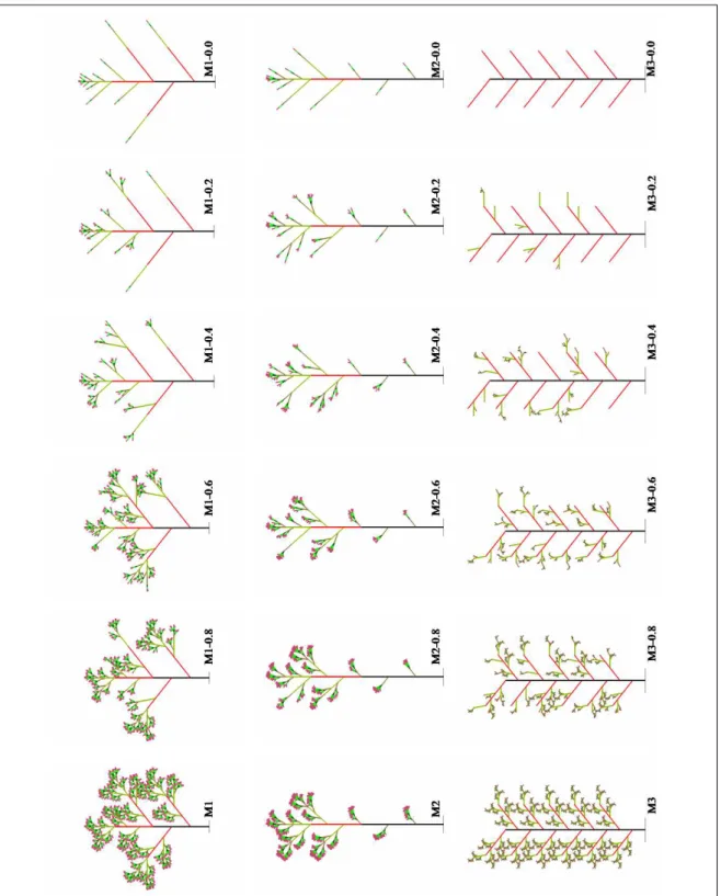
The differentiation graph of each plant has seven states, with 1 denoting the initial state and 7 denoting the terminal (flowering) state. A family Mi consists of a determin-istic model Mi and five derived models. The differentiation graphs of the determindetermin-istic models M1, M2 and M3 are shown in Fig. 7. In model M1, the lateral meristems that are generated by an apical meristem in state s have state s + 1. The state of the apical meristem remains unchanged for the given number of steps, then advances by 1 (except for the final state). Model M2 differs from M1 in that some lateral meristems produced by the apical meristem in state s may assume state s′
greater than s + 1. For example, the apical meristem in state 1 produces a lateral meristems in state 3. In model M3, a meristem in state s produces lateral meristems in state s′
= s + 1, but there is no gradual progression of states along either the main or the lateral axes. Instead, after remaining in the same state for a number of steps, an apical meristem differentiates directly into a flower.
For each deterministic plant Mi, we generated a set of five derived plants, labeled M i− 0.8, Mi − 0.6, . . . , Mi − 0.0, by randomizing the functioning of the lateral meristems. With probability p, a lateral apex of order greater than 2 gave rise to a branch; otherwise, the branch was aborted. This probability p is indicated in the plant name: p = 0.8 in M i− 0.8, p = 0.4 in Mi − 0.4, and so on. First-order branching was not affected by this probability.
the main shoot structure; thus, structures M1 and M2 are self-similar in the sense of Definition 4 (Fig. 8). The random removal of branches in these structures introduces variation that is expected to reduce their degree of self-similarity. In contrast, the lateral branches of M3 are not copies of the main structure; thus, M3 is not self-similar, and its random variations are also not expected to be self-similar. Below we show how these qualitative characterizations are captured and quantified by the self-similarity parameters.
3.2
Analyzing and Comparing Self-Similarity of Theoretical Plants
The data were analyzed using the AMAPmod module for plant architecture analysis,31
which incorporates algorithms for comparing tree graphs.24 AMAPmod is a part of the
ALEA modeling platform.32
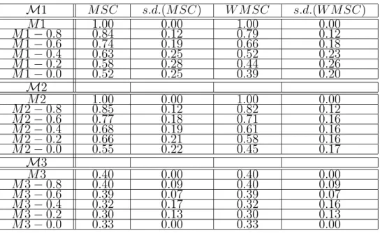
The unweighted and weighted mean self-similarity coefficients, and the variance of unweighted and weighted paracladial coefficients, were computed for each plant of the three families M1, M2 and M3. The results are given in Table 1.
We observe that the MSC (mean self-similarity coefficient) of plants M1 and M2 is equal to 1. This indicates perfect self-similarity, which is consistent with the manner in which these plants were generated. In contrast, the MSC of plant M3 is equal to 0.4, which means that for each branch borne by the trunk, an average of 60 percent of its components should be added, removed, or rearranged to achieve the self-similarity condition of Proposition 5. This low value of the MSC is again consistent with the manner in which plant M3 was generated, since its simulation algorithm explicitly prevented the lateral branches from following the structure of their parent.
Within the randomized plant families M1 and M2, the reduction of the branching probability p is followed by a reduction in the value of MSC. This is consistent with our expectation that removing branches at random from an initially self-similar structure will decrease its self-similarity. In the family M3, in contrast, the overall decrease of the MSC from 0.4 for plant M3 to 0.3 for plant M3 − 0.0 is not monotonic. This suggests that
randomly removing branches in a non-self-similar plant may either increase or decrease its self-similarity.
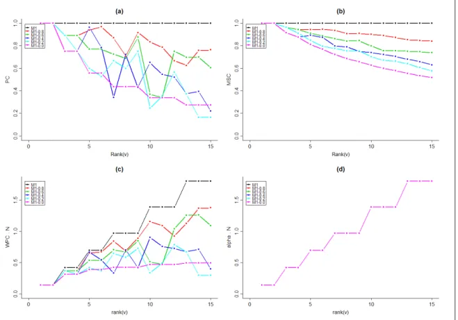
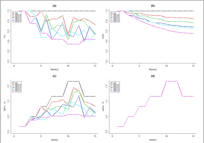
Profile curves provide an additional characterization of plant architecture. The profile of the paracladial coefficients γ(v) for the reference plant M1 (top curve in Fig. 9.a) shows that its branches are strictly paracladial: γ(v) = 1 for all positions v. This is consistent with the definition of M1 as a perfectly self-similar plant. In the randomized plants M1 − 0.8 . . . , M1 − 0.0, the edit distance between branches and the trunk tends to increase for branches positioned lower on the trunk. Although in Fig. 9.a this trend is obscured by the random variation of the paracladial coefficients γ(v), it is clearly visible in Fig. 9.b, which shows the self-similarity coefficients γ(r). The gradual decrease in the values of the paracladial coefficient and the self-similarity coefficient as rank(v) increases reflects the dependence of both coefficients on the size of branches: the lower branches in the plant family M1 are larger than the upper branches (Fig. 8, first row), and therefore more likely to depart from the trunk structure.
The weighted paracladial coefficients γ′
(v) were introduced to compensate for this apparent overemphasis of the self-similarity of small branches. The values of γ′
(v) for the plant family M1 are shown in Fig. 9.c; the lengths of branches that serve as weights are plotted in Fig. 9.d. As expected, we observe an increase in the value of γ′
(v) proportional to the size of branches in the self-similar plant M1. This increase is less pronounced in the randomized plants.
The corresponding profiles for the plant family M2 are shown in Fig. 10. We observe that the paracladial coefficient γ(v) reaches a minimum for the longest lateral branches with the rank(v) = 10, 11, 12, but the weighted paracladial coefficient γ′
(v) reaches its maximum for the same branches. The use of weights can thus qualitatively affect our assessment of the contribution of individual branches to the self-similarity of the whole plant structure.
The profiles for family M3 (Fig. 11) have a distinctly different character from the profiles of families M1 and M2, which reflects the non-self-similar character of plants in
M3.
4
APPLICATION TO REAL PLANTS
4.1
Plant Material
We considered branching structures of two plant parts with marked self-similar organiza-tion: lilac inflorescences and rice shoots.
Five Syringa vulgaris (common lilac) inflorescences were collected and measured in Calgary Canada, in the spring of 2001. In addition to the topological structure (map) of these inflorescences, the length and the diameter of each internode, and the length and diameter of each flower were measured using a digital caliper connected to a computerized data collection system.15 This made it possible to reconstruct these inflorescences with
great accuracy (Fig. 12). In the present study, we only used topological data. Since lilac inflorescences have two branches at each node, we averaged the paracladial coefficients of both branches to define a single value at each node on the paracladial coefficient profiles. The second plant was an Oryza sativa (rice) cv ‘Nippon Bare’ plant, which has more complex lateral structures (reiterated systems33) than the lilac inflorescences. The
topo-logical structure of an individual plant was completely mapped, including vegetative and floral parts.34 Figure 13 shows a picture of this individual and its corresponding schematic
representation. The structure is made of a main axis bearing a main inflorescence (pan-icle) and four lateral reiterated systems (called tillers), each composed of a vegetative part and one inflorescence. The tillers themselves bear lateral axes, some of them bearing inflorescences. This gave us the opportunity to evaluate the self-similarity of both the inflorescences and the vegetative parts.
4.2
Results
4.2.1 Lilac
Lilac inflorescences have high coefficients of self-similarity (average 0.92, Table 2). This MSC value is comparable to that of the randomized theoretical plants in families M1 and M2, though it is higher than even that of the least randomized plants M1 − 0.8 and M2 − 0.8.
For all inflorescences, the paracladial coefficients of the first-order branches up to rank 6 (from the tip) are very close to one. The coefficients then slowly decrease to 0.6 (Fig. 14.a). The mean values of these coefficients range between 0.89 and 0.94 over the five inflorescences, with a low standard deviation (close to 10% on average, Table 2). This reveals a very homogeneous self-similar nature of these inflorescences, as confirmed by the almost perfectly superimposed MSC profiles (Fig. 14.b).
The weighted paracladial coefficients relate the paracladial coefficients to the complex-ity of branches. As shown in Fig. 14.c, the values of WPC tend to increase up to rank 9, where they stabilize around a constant value. From rank 9 on, the decrease in the value of (unweighted) paracladial coefficients is thus compensated by the fact that the structures become more complex.
To visualize these results in a more intuitive manner, we colored the branches of the reconstructed lilac inflorescences according to the values of their unweighted or weighted paracladial coefficients. If the unweighted paracladial coefficients are used (Fig. 15), the most self-similar part of each inflorescence is situated near its top, where the branches are short. Weighted paracladial coefficients compensate for this bias toward the short branches, giving a different perspective of the distribution of self-similarity within the inflorescences (Fig. 16). Contribution to self-similarity is now low at the tips, while the branches that most contribute to self-similarity are located in the medial and basal parts of the inflorescences.
• The degree of self-similarity of the five lilac inflorescences is high (average 0.92).
• The self-similar nature of these inflorescences is very homogeneous.
• A stable trade-off between paracladial quality and complexity of lateral inflores-cences is reached in the basal part of these plants (after rank 9).
• The 3D representation of paracladial coefficients gives a very intuitive visual indi-cation of the contribution of each branch to the plant’s overall self-similarity.
4.2.2 Rice
The topology of rice is rather complex since it contains inflorescences (panicles), vegetative parts, and reiterated systems. This gave us the opportunity to compare the self-similarity of both inflorescences and vegetative parts.
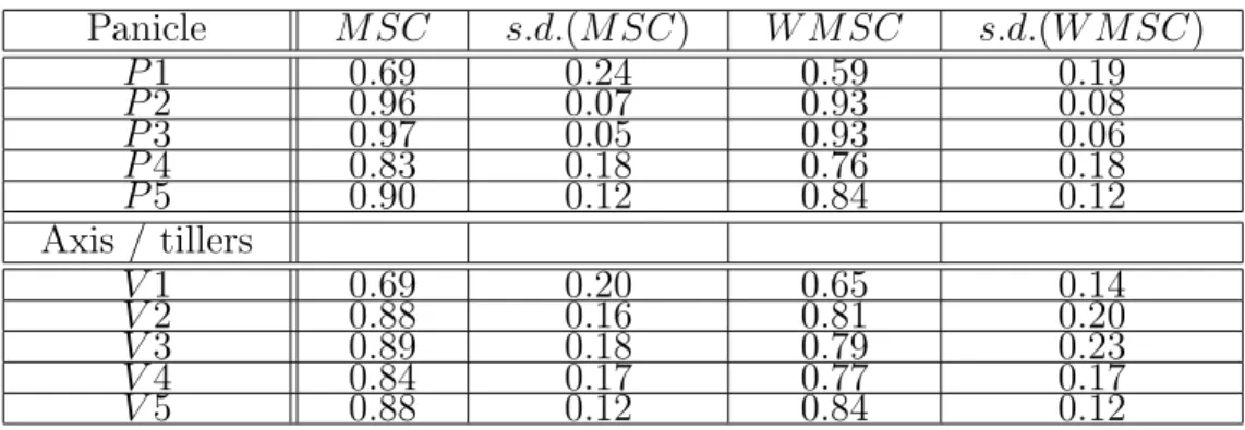
We first analyze the self-similarity of plant panicles P 1 − P 5 (Fig. 17, ranks 1-11). Their similarity coefficients show that the two basal panicles are highly self-similar (MSC equal to 0.96 and 0.97), whereas the two intermediate panicles have lower coefficients (0.90 and 0.83) (Table 3). The main stem panicle has a much lower MSC (0.69), because its axis carries long branches with relatively low paracladial coefficients, located near the tip of this panicle (Fig. 17.a).
The panicles have relatively lower paracladial coefficients in their medial parts. At the base of the panicles the paracladial coefficients of P 2, P 4 and P 5 become much higher (Fig. 17.a). The length of the lateral branches in the panicles tends, however, to vary in the opposite way: it is high in the medial part, and lower at the base (Fig. 17.d). The superposition of these trends results in high and relatively constant weighted paracladial coefficients for all branches up to rank 11 (Fig. 17.c).
Now let us take into account the vegetative parts of the plants in the evaluation of self-similarity. On Fig. 17.a, ranks 1-21, we observe that the paracladial coefficients of all axes tend to decrease in proximal positions with respect to the panicle base, except for the
main axis (V 1), for which the opposite tendency is observed. Due to the important length of tillers, this phenomenon is even more marked on the weighted paracladial coefficients (Fig. 17.c).
The tillers themselves vary in their self-similar nature. V 2, V 4, and V 5 have similar structure for their distal part (up to rank 15) (Fig. 17.c). However, unlike V 4 and V 5, V2 bears a secondary tiller, which makes it more similar to the trunk and thus greatly increases its overall weighted paracladial coefficient on the basal part, to the level of V 3. This leads V 2 and V 3 to exhibit nearly identical coefficients of self-similarity.
From this analysis, we conclude that:
• The tiller panicles are more self-similar than the apical panicle (Fig. 17.b).
• The degree of self-similarity of the tiller panicles is high (average 0.92)
• The degree of self-similarity of the whole tillers is also high (average 0.87)
• The degree of self-similarity of the entire plant is relatively lower (0.69). This is mainly due to the lack of self-similarity in the main stem panicle.
• Nevertheless, the tillers are highly similar to the main stem structure (Fig. 17.c). This supports the idea that tillers can be viewed as reiterated complexes of the plant.
5
CONCLUSION
This paper addressed the problem of quantifying the degree of self-similarity in branching plant structures. To this end, we introduced the notions of paracladial coefficient and mean self-similarity coefficient for axial trees. The paracladial coefficient characterizes the similarity between an individual branch and the main stem of the structure, whereas the mean self-similarity coefficient provides a global measure of the self-similarity of the entire structure. Weighted coefficients were also introduced to take into account the size
of branches while quantifying self-similarity. These definitions have been applied to both simulated branching structures and real plants. The simulated structures were used to illustrate main characteristics of the proposed measures. Real plants were used to show that these measures are appropriate for interpreting experimental data.
For over fifty years, botanists have postulated that describing a plant as an assembly of similar parts plays a key role in the understanding of plant structure and development. The formalization and quantification of self-similarity of plant structure may contribute to this understanding. Insights from the study of self-similarity may also assist in the construction of simulation plant models, by exposing the repetitive elements of plant architecture. Furthermore, the use of self-similarity may lead to significant simplifications of plant mapping and measurement techniques, since parts known to be similar to other parts need not be measured.
The definition of self-similarity proposed in this paper is well adapted to the analysis of monopodial plants (with a clearly defined main axis or trunk). Its extensions to sym-podial plants, and to alternative definitions of plant self-similarity15, 16 need to be further
investigated.
6
ACKNOWLEDGMENT
The authors thank Lars M¨undermann for collecting the data on lilac inflorescences, Yves Caraglio and Clo´e Paul-Victor for kindly providing us the data on rice, and Brendan Lane for insightful comments and editorial help.
References
[1] F. Hall´e, R. Oldeman, and P. Tomlinson, Tropical trees and forests. An architectural analysis, Springer Verlag, New York, 1978.
[3] J. L. Harper, Population biology of plants, Academic Press, London, 1977.
[4] D. Barth´el´emy, Acta Biotheoretica 39, 309 (1991).
[5] P. M. Room, L. Maillette, and J. Hanan, Advances in Ecological Research 25, 105 (1994).
[6] C. Godin and Y. Caraglio, Journal of Theoretical Biology 191, 1 (1998).
[7] P. de Reffye, C. Edelin, J. Fran¸con, M. Jaeger, and C. Puech, Plant models faithful to botanical structure and development, in SIGGRAPH 1988 Conference Proceedings, pages 151–158, Atlanta, GA, 1988, ACM Press, New York.
[8] P. Prusinkiewicz and A. Lindenmayer, The algorithmic beauty of plants, Springer Verlag, New York, 1990.
[9] B. B. Mandelbrot, The fractal geometry of nature, W. H. Freeman, San Francisco, 1982.
[10] A. Arber, Natural philosophy of plant form, University Press, Cambridge, 1950.
[11] W. Troll, Die Infloreszenzen, volume 1, Gustav Fisher Verlag, 1964.
[12] C. H. Schultz, Neues System der Morphologie der Pflanzen, Berlin, 1847.
[13] D. Frijters and A. Lindenmayer, Developmental descriptions of branching patterns with paracladial relationships., in Automata, languages, development, edited by A. Lindenmayer and G. Rozenberg, pages 57–73, North-Holland, Amsterdam, 1976.
[14] P. Prusinkiewicz, L. M¨undermann, R. Karwowski, and B. Lane, The use of positional information in the modeling of plants, in SIGGRAPH 2001 Conference Proceedings, pages 289–300, Los Angeles, CA, 2001, ACM Press, New York.
[16] P. Prusinkiewicz, Self-similarity in plants: Integrating mathematical and biological perspectives, in Thinking in patterns. Fractals and related phenomena in nature, edited by M. Novak, pages 103–118, World Scientific, New Jersey, 2004.
[17] A. Lindenmayer, Journal of Theoretical Biology 18, 280 (1968).
[18] G. Herman, A. Lindenmayer, and G. Rozenberg, Mathematical Systems Theory 8, 316 (1975).
[19] L. Gatsuk, O. Smirnova, L. Zaugolnova, and L. Zhukova, Journal of Ecophysiology 68, 675 (1980).
[20] R. Nozeran, Integration of organismal development, in Positional control in plant development, edited by P. W. Barlow and D. Carr, pages 375–401, Cambridge Uni-versity Press, 1984.
[21] D. Barth´el´emy, Y. Caraglio, and E. Costes, Architecture, gradients morphog´en´etiques et ˆage physiologique chez les v´eg´etaux, in Mod´elisation et simulation de l’architecture des v´eg´etaux, edited by J. Bouchon, P. de Reffye, and D. Barth´el´emy, pages 11–87, Inra ´Editions, Paris, 1997.
[22] P. de Reffye, P. Dinouard, and D. Barth´el´emy, Architecture et mod´elisation de l’orme du Japon Zelkova serrata (Thunb.) Makino (Ulmaceae): la notion d’axe de r´ef´erence, in De la forˆet cultiv´ee `a l’industrie de demain: 3e colloque Sciences et Industries du Bois, Arbora, pages 351–352, Bordeaux, France, 1991.
[23] K. Zhang, Algorithmica 15, 205 (1996).
[24] P. Ferraro and C. Godin, Annals of Forest Science 57, 445 (2000).
[25] P. Ferraro and C. Godin, Algorithmica 36, 1 (2003).
[26] A. D. Bell, Plant form, an illustrated guide to flowering morphology, Oxford Univer-sity Press, Oxford, U.K., 1991.
[27] A. Ohmori and E. Tanaka, Syntactic and Structural Pattern Recognition 45, 85 (1988).
[28] K. Zhang and T. Jiang, Information Processing Letters 49, 249 (1994).
[29] R. Mech, R. Karwowski, and B. Lane, Cpfg version 4.0 user’s manual, 2004, De-partment of Computer Science, University of Calgary, Alberta, Canada. Available at http://www.algorithmicbotany.org/lstudio/CPFGman.pdf.
[30] P. Prusinkiewicz, Acta Horticulturae 630, 15 (2004).
[31] C. Godin, Y. Gu´edon, and E. Costes, Agronomie 19, 163 (1999).
[32] C. Pradal et al., ALEA: A software for integrating analysis and simulation tools for 3D architecture and ecophysiology, in Proceedings of the 4th International Workshop on Functional-Structural Plant Models, FSPM04, edited by C. Godin et al., pages 406–407, Montpellier, France, 2004, UMR AMAP.
[33] D. Barth´el´emy, C. Edelin, and F. Hall´e, Canopy architecture, in Physiology of trees, edited by A. Raghavendra, pages 1–20, John Wiley & Sons, 1991.
[34] C. Paul-Victor, Diversit´e morphologique et architecturale de quatre vari´et´es de riz (Oryza sativa et Oryza glaberrina), Master’s thesis, University of Jussieu, Paris 6, 2004.
7
APPENDIX
Proof of Proposition 5: An axial tree T = (V, E, α) rooted in r is self-similar if and only if ∀v ∈ B(r), T [v] is a paracladium.
The “if” part of the proof. We assume that any branch B1 with the base v originating at
with some distal portion T1 of T (Fig. 4). We want to show that for every vertex w of T ,
the branch T [w] rooted in w is also isomorphic with some distal portion of T . Proof by induction on the order n of vertex w.
1. Initial step. If n = 0, the vertex w lies on the main axis of T , and the subtree T [w] is the distal portion of T rooted in w.
2. Inductive step. Assume that the proposition holds for some n ≥ 0, and consider a vertex w of order n + 1. The branch T [w] rooted in w is included in some branch T[v], where v is a vertex of order n. From the inductive assumption it follows that T[v] is isomorphic with some distal portion T1 of T . The image of T [w] under this
isomorphism is a (distal portion of) some first-order branch B1, which, according to
the assumption of the “if” part of the proof, is isomorphic with some distal portion T2 of T . By transitivity of isomorphisms, T [w] is also isomorphic with T2.
The “only if” part of the proof. We assume that any branch B rooted in some vertex w in T is isomorphic with some distal portion T1 of T . In particular, any branch B1 with
Tables
M1 M SC s.d.(MSC) W M SC s.d.(W MSC) M1 1.00 0.00 1.00 0.00 M1 − 0.8 0.84 0.12 0.79 0.12 M1 − 0.6 0.74 0.19 0.66 0.18 M1 − 0.4 0.63 0.25 0.52 0.23 M1 − 0.2 0.58 0.28 0.44 0.26 M1 − 0.0 0.52 0.25 0.39 0.20 M2 M2 1.00 0.00 1.00 0.00 M2 − 0.8 0.85 0.12 0.82 0.12 M2 − 0.6 0.77 0.18 0.71 0.16 M2 − 0.4 0.68 0.19 0.61 0.16 M2 − 0.2 0.66 0.21 0.58 0.16 M2 − 0.0 0.55 0.22 0.45 0.17 M3 M3 0.40 0.00 0.40 0.00 M3 − 0.8 0.40 0.09 0.40 0.09 M3 − 0.6 0.39 0.07 0.39 0.07 M3 − 0.4 0.32 0.17 0.32 0.16 M3 − 0.2 0.30 0.13 0.30 0.13 M3 − 0.0 0.33 0.00 0.33 0.00Table 1: Self-similarity coefficients and their standard deviation for plant families M1, M2 and M3 M SC s.d.(MSC) W M SC s.d.(W MSC) A1 0.89 0.13 0.82 0.10 A2 0.94 0.08 0.82 0.06 A3 0.89 0.12 0.83 0.09 A4 0.93 0.10 0.88 0.07 A5 0.92 0.09 0.86 0.07
Panicle M SC s.d.(MSC) W M SC s.d.(W MSC) P1 0.69 0.24 0.59 0.19 P2 0.96 0.07 0.93 0.08 P3 0.97 0.05 0.93 0.06 P4 0.83 0.18 0.76 0.18 P5 0.90 0.12 0.84 0.12 Axis / tillers V1 0.69 0.20 0.65 0.14 V2 0.88 0.16 0.81 0.20 V3 0.89 0.18 0.79 0.23 V4 0.84 0.17 0.77 0.17 V5 0.88 0.12 0.84 0.12
Table 3: Self-similarity coefficients and their standard deviation for rice panicles, the whole main axis V 1, and tillers V 2 − V 5
Figures
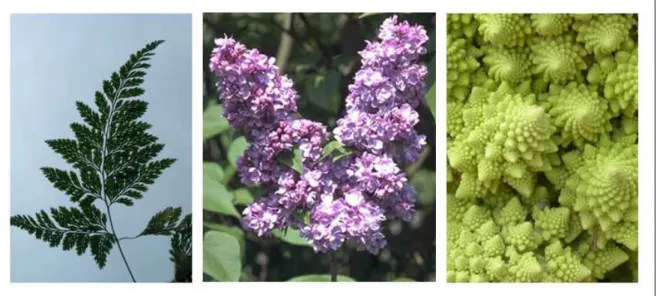
Figure 1: Examples of plants showing remarkably self-similar branching structures: a fern leaf, a compound inflorescence (lilac), and a romanesco broccoli.
Figure 2: Different sub-structures and sets in an axial tree. a) Visualization using a schematic plant representation. b) Visualization using the equivalent axial tree represen-tation. c) Definition of the set B(r) for an axial tree T [r].
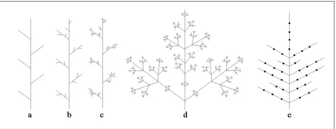
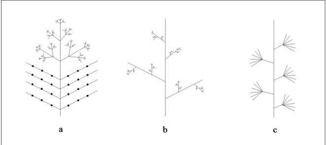
Figure 3: Perfectly self-similar branching structures with different maximum branching orders (equal to 1,2,3,4 and 1, a to e) and different apparent complexity.
Figure 4: The recursive principle of self-similarity in plants. a) A visualization using a single branching structure. b) A visualization using a general representation of branching structures.
Figure 5: a) Two tree structures of the same size with maximum topological distance. b) Two different tree structures that are isomorphic if axial information is not taken into account, but non-isomorphic otherwise.
Figure 6: Examples of non-similar structures. a) The upper part is perfectly self-similar and the basal part is not. b) The basal part is perfectly self-self-similar and the upper part is not. c) An extremely non-self-similar structure. The paracladial coefficient γ(v) of each comb-like branch is equal to 2
n+2, where n is the number of components in the
Figure 7: Differentiation graphs used for defining theoretical plants. a) The differentiation graph of non-branching growth. b) The resulting axis structure, where component colors correspond to the differentiation graph states in which these components were created. The numbers attached to each loop indicate the number of steps a meristem stays in the corresponding state. M1, M2, M3) The differentiation graphs of models M1, M2, and M3. Solid arrows correspond to possible transitions of the apical meristem states. Dashed arrows correspond to possible transitions from the apical meristem state to the axillary meristem states.
Figure 8: Theoretical plants: the M1 family (first row), the M2 family (second row), and the M3 family (third row).
Figure 9: Profiles of PC, WPC ·N, MSC and α · N for theoretical plants M1. Both WPC and α profiles have been multiplied by the number of branches in the plant, denoted by N.
Figure 12: One of the lilac inflorescences used in the analysis of self-similarity and its 3D reconstruction .14
Figure 13: a) Oryza sativa cv ‘Nippon Bare’ (rice) individual (Photo: Clo´e Paul Victor). b) Schematic representation of the individual topological structure, showing one main axis and four lateral tillers. Vegetative parts are in green and inflorescences are in red. Flowers are represented as ovoid black shapes. Leaves are not represented. Labels identify the different analyzed branching structures and are located at the base of the corresponding structures.
Figure 14: Profiles of PC, WPC ·N, MSC and α · N for lilac inflorescences.
Figure 15: False color illustrations of lilac inflorescences showing the value of the para-cladial coefficient (PC).
Figure 16: False color illustrations of lilac inflorescences showing the value of the weighted paracladial coefficient (WPC).