Characterization and analysis of highly diagonal Terahertz Quantum Cascade Lasers

(1)

Characterization and Analysis of Highly Diagonal

Terahertz Quantum Cascade Lasers

by

Chun Wang Ivan Chan

Submitted to the Department of Electrical Engineering and Computer

Science

in partial fulfillment of the requirements for the degree of

Master of Science in Electrical Engineering

at the

MASSACHUSETTS INSTITUTE OF TECHNOLOGY

September 2010

c

° Massachusetts Institute of Technology 2010. All rights reserved.

Author . . . .

Department of Electrical Engineering and Computer Science

August 25, 2010

Certified by . . . .

Qing Hu

Professor

Thesis Supervisor

Accepted by . . . .

Terry P. Orlando

Chairman, Department Committee on Graduate Theses

(2)

(3)

Characterization and Analysis of Highly Diagonal Terahertz

Quantum Cascade Lasers

by

Chun Wang Ivan Chan

Submitted to the Department of Electrical Engineering and Computer Science on August 25, 2010, in partial fulfillment of the

requirements for the degree of Master of Science in Electrical Engineering

Abstract

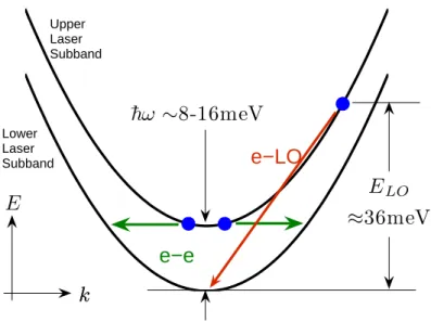
The as yet unattained milestone of room-temperature operation is essential for es-tablishing Terahertz Quantum Cascade Lasers (THz QCLs) as practical sources of THz radiation. Temperature performance is hypothesized to be limited by upper laser level lifetime reduction due to non-radiative scattering, particularly by longi-tudinal optical phonons. To address this issue, this work studies highly “diagonal” QCLs, where the upper and lower laser level wavefunctions are spatially separated to preserve upper laser level lifetime, as well as several other issues relevant to high temperature performance.

The highly diagonal devices of this work performed poorly, but the analysis herein nevertheless suggest that diagonality as a design strategy cannot yet be ruled out. Other causes of poor performance in the lasers are identified, and suggestions for future designs are made.

Thesis Supervisor: Qing Hu Title: Professor

(4)

(5)

Acknowledgments

Many are those whom I must thank. I thank my supervisor Professor Qing Hu for his guidance and support over the last two years. I thank Dr. Sushil Kumar for this invaluable tutelage; I aspire to his patience, should the day come when I am called to teach as well. I also thank my lab mates Dr. Alan Lee, Qi Qin, Wilt Kao, and David Burghoff for being an excellent gang of friends, ever ready to share in jokes and ideas. I am both humbled and honored to share in the company of so much good will and talent. Additionally, I thank Dr. John Reno at Sandia National Laboratories for the MBE growth crucial to this work.

Outside of academia, I am indebted to my family for a quarter-century of unwaver-ing love and support. In particular, if I have succeeded at all in life, I owe everythunwaver-ing to my grandmother, Sik-Je Lam, who unfortunately passed away February of this year; I will never forget her.

Finally, I gratefully acknowledge funding from NASA, the primary sponsor of this research, and the National Science and Engineering Research Council of Canada, who provided me with my first year scholarship.

(6)

(7)

List of Figures

1-1 The “terahertz gap” in the electromagnetic spectrum . . . 15

1-2 Subband transitions in a heterostructure. . . 17

1-3 Schematic of QCL operation. . . 17

2-1 Schematic of miniband conduction . . . 25

2-2 Schematic of Wannier-Stark hopping conduction . . . 26

2-3 Extended versus localized bases for heterostructures. . . 30

2-4 Schematic of a pseudospectral differentiation matrix for the spectral element method. . . 43

3-1 Sample band diagrams of CSL and BTC designs. . . 63

3-2 Sample band diagram of an FL family device . . . 65

3-3 Sample band diagram of an OWI family device . . . 66

3-4 Sample band diagram of an DSL family device . . . 68

3-5 Non-radiative scattering mechanisms between upper and lower laser subbands. . . 69

3-6 Injector-collector resonance (lower level parasitic). . . 73

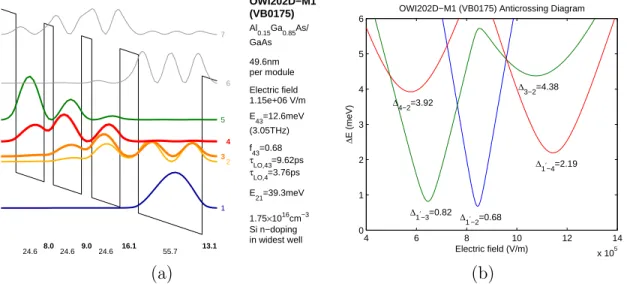
4-1 Design parameters for OWI202D-M1 . . . 86

4-2 Experimental results for OWI202D-M1 . . . 87

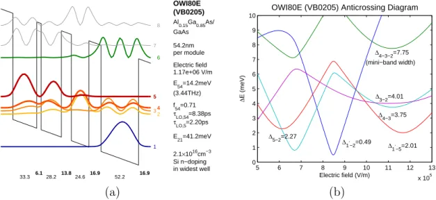
4-3 Design parameters for OWI180E . . . 88

4-4 Experimental results for OWI180E . . . 89 4-5 Design parameters for OWI185E-M1 (resonant tunneling injection) . 91

(10)

4-6 Proposed 7-4 versus 5-4 scattering assisted injection mechanisms in

OWI185E-M1 . . . 92

4-7 7-4 versus 5-4 scattering assisted injection rates in OWI185E-M1 . . . 93

4-8 Experimental results for OWI185E-M1 . . . 94

4-9 Design parameters for 3-well design of Luo et al., APL 2007 . . . 95

4-10 Design parameters for OWI222G . . . 95

4-11 Experimental results for OWI222G . . . 96

4-12 Experimental results for OWI222G . . . 97

4-13 Figure-of-merit comparison between OWI222G and Luo APL 2007 3-well design . . . 98

4-14 Design parameters for TW246 . . . 99

4-15 Experimental results for TW246 . . . 100

4-16 Figure-of-merit comparison between TW246 and OWI222G . . . 101

4-17 Hot phonon absorption in TW246. . . 103

4-18 Design parameters for OWI190E-M2 . . . 105

4-19 Experimental results for OWI190E-M2, VB0288 . . . 106

4-20 Experimental results for OWI190E-M2, VB0287 . . . 107

4-21 Scattering assisted injection mechanisms in OWI185E-M1 . . . 109

4-22 Scattering assisted injection rates in OWI190E-M2 . . . 110

4-23 Design parameters for OWI222G-M1 . . . 110

4-24 Experimental results for OWI222G-M1 . . . 111

4-29 Comparison of OWI235G-M3 and OWI222G non-lasing IV s . . . 117

4-30 Design parameters for TW260-M1 . . . 118

4-31 Experimental results for TW260-M1 . . . 119

4-32 Design parameters for TP3W200 . . . 121

(11)

4-34 Design parameters for TP4W160 . . . 123

4-35 Experimental results for TP4W160 . . . 124

4-36 Design parameters for FL190S-M2 . . . 125

4-37 Experimental results for FL190S-M2 . . . 126

4-42 Design parameters for OWI210H . . . 134

4-43 Experimental results for OWI210H, VB0373 . . . 135

4-44 Experimental results for OWI210H, VB0364 . . . 137

4-45 Design parameters for OWI209H-M1 . . . 138

4-46 Experimental results for OWI209H-M1 . . . 139

4-47 Design parameters for OWI208H-M2, VB0393 . . . 140

4-48 Experimental results for OWI208H-M2, VB0393 . . . 141

4-49 Design parameters for OWI208H-M2, VB0385 . . . 142

4-50 Experimental results for OWI208H-M2, VB0385 . . . 143

4-51 Design parameters for SDIP2W . . . 144

4-52 Experimental results for SDIP2W . . . 145

4-53 Design parameters for SDRP4W . . . 146

4-54 Experimental results for SDRP4W . . . 147

4-55 Design parameters for SDRP5W . . . 149

(12)

(13)

List of Tables

2.1 Performance of custom spectral element code vs. SEQUAL 2.1 (finite difference code) . . . 45

(14)

(15)

Chapter 1 Introduction

The two major sources of coherent radiation in modern technologies are electronic os-cillators and conventional lasers. The need for explicit charge transfer limits electronic oscillators via RC time constants to approximately <300GHz. Conversely, naturally occurring bandgaps tend not to fall below ∼60meV (eg. in lead-salt lasers [1]), lim-iting conventional lasers to approximately >15THz. The source-poor region of the spectrum lying in ∼0.3THz–10THz is therefore known as the terahertz gap (see figure 1-1). Diverse applications ranging from chemical sensing and spectroscopy to security and astronomical imaging have been proposed for the THz spectrum (see, for exam-ple, [2–6]), thus it remains desirable to find compact sources of continuous-wave, high power, coherent THz radiation.

Figure 1-1: The “terahertz gap” in the electromagnetic spectrum. Few natural sources of radiation exist in this range.

(16)

oscillators and Schottky-diode frequency multipliers provide output powers only of order ∼10µW [7, 8]. Solid-state lasers based on strained p-type germanium with crossed electric and magnetic fields or optically pumped impurity state transitions in silicon require liquid helium operating temperatures and permit only pulsed operation due to large energy consumption and poor efficiency [9]. Optically pumped molecular gas lasers based on vibrational/rotational molecular state transitions are bulky and energy inefficient, and moreover yield only a limited number of frequencies (although they have seen some practical use [10]). Free electron lasers offer high power and broad tuning, but are even more unwieldy; they remain impractical outside of research due to large cost, size, and infrastructure requirements.

The topic of this thesis is the Quantum Cascade Laser (QCL), arguably the most promising THz source currently under development.

1.1 Quantum Cascade Lasers

At heart, a QCL is a superlattice. First proposed by Esaki and Tsu in 1970 [11], a superlattice is a periodic stack of semiconductor films of varying thicknesses that is typically grown by molecular beam epitaxy (MBE). At the heterojunctions boundaries between different semiconductor layers, the abrupt change in lattice potential creates discontinuities in the conduction band-edge energies, leading to quantum confinement in the growth direction. This splits the material conduction band states into subbands, between which optical transitions can occur (see figure 1-2).

Kazarinov and Suris first proposed the basic idea of a QCL in 1971 [12]: through careful selection of layer widths, a biased superlattice can achieve optical gain through population inversion between subband states. Referring to figure 1-3, a single elec-tron can “cascade” in energy down the superlattice while emitting a photon in each superlattice period, ingeniously enabling effective quantum efficiencies much higher than unity (in principle).

The first QCL was demonstrated in 1994, lasing in the mid-infrared (mid-IR) [13]. Mid-IR QCLs have since advanced rapidly in power, efficiency, and maximum lasing

(17)

Figure 1-2: Electronic transitions in a heterostructure. The abrupt material discon-tinuity leads to both conduction and valence band energy level discretizations in the well region. ~ω1 is an intersubband transition, on which QCLs are based, and ~ω2 is

an interband transition, on which traditional semiconductor lasers are based.

Figure 1-3: Schematic of QCL operation. In principle, each electron emits one photon in each superlattice period before moving into the next period.

(18)

temperature [14], establishing themselves in diverse applications such as spectroscopy and optical communications [15]. K¨ohler et al. demonstrated the first operational THz QCL in 2002 [16]. THz QCLs now cover the spectral range from 5THz down to 1.2THz (or even lower with magnetic field assistance [17, 18]), and can emit up to hundreds of milliwatts of power.

1.2 THz QCL Temperature Performance

Unfortunately, THz QCLs have in general lagged behind their mid-IR counterparts in progress; perhaps the eight year gap between the first mid-IR QCL and the first THz QCL attests to the difficulty of working in the THz regime. The foremost barrier to application is that THz QCLs require cryogenic operation. Whereas mid-IR QCLs have long ago attained continuous-wave room temperature operation [19], no THz QCL to date operates above 186K (see design OWI222G in section 4.2.5, and also [20]). This thesis details theoretical and experimental investigations into the limits to temperature performance and progress made towards achieving higher temperature operation.

The postulated limit to high temperature performance is degradation of popula-tion inversion due to non-radiative scattering. With increasing temperature, scat-tering mechanisms (most notably interactions with LO phonons) cause upper laser subband electrons to transit to the lower laser subband without photon emission. Section 3.2.1 later in this thesis elaborates further on this topic.

Solutions such as magnetic confinement [18, 21], zero-dimensional heterostruc-tures [22], and new material systems (in particular, GaAsN [23]) have been proposed in the literature to quench non-radiative scattering mechanisms. In particular, mag-netic confinement has already proven capable of raising operating temperatures to 225K, but the equipment needed to generate the requisite ∼10-16T magnetic fields is even less practical than cryogenic cooling equipment. Adequate zero-dimensional het-erostructures have yet to be fabricated, and epitaxial growth in GaAsN is notoriously difficult [24].

(19)

As an alternative, the MIT THz QCL group of Professor Qing Hu is pursuing the less radical strategy of increasing the spatial separation between upper and lower laser level wavefunctions, or the so-called “ diagonality” of the laser design. While high diagonality carries its own disadvantages, calculated scattering rates indicate that diagonality ensures the survival of population inversion up to room temperatures. The thesis explores the effects of diagonality on THz QCL design, particularly on observed experimental transport properties.

1.3 Thesis Overview

The remainder of this thesis is organized as follows.

• Chapter 2 expands upon the qualitative introduction given in this chapter,

explaining the physical models of QCL transport.

• Chapter 3 draws upon the theoretical foundation formed in chapter 2 to discuss

QCL design.

• Chapter 4 presents the analysis and experimental data for the devices studied,

(20)

(21)

Chapter 2 The Theory of Quantum Cascade

Laser Operation

Although conceptually easy to understand, QCL operation is challenging to model quantitatively. This is because electrical transport in a QCL is neither fully ballistic nor fully scattering-assisted, so traditional approaches such as Landauer-Buttiker transmission and the drift-diffusion equations do not apply. This chapter details the semiclassical/quantum phenomenological methods that have been adapted for QCL analysis. One must bear in mind that these methods, although useful, are highly approximate.

In recent years, much effort has been devoted to the development of fully quantum mechanical theories of transport in the formalism of Nonequilibrium Green’s

Func-tions (NEGF; see for example [25, 26]). This field of research is promising, but the

tremendous computational burden of NEGF prevents its regular use in design, and even the best implementations presently available do not make consistently accurate predictions.

There are two crucial transport processes which must be considered in detail: carrier scattering and resonant tunneling.

(22)

2.1 The Envelope Function Approximation (EFA)

for Superlattices

Quantum cascade lasers are typically analyzed using effective-mass theory in the envelope function approximation. There is extant work on QCL modeling using more accurate microscopic approaches, such as the tight-binding approximation [27], but the envelope function approximation remains invaluable for its simplicity and ability to give rapid results.

The governing equation is the effective mass envelope function equation that de-termines the wavefunction envelope F (r),

−∇ ~

2

2m∗_(r)∇F (r) + V (r) F (r) = EF (r) (2.1)

where m∗_{(r) is a spatially varying effective mass encoding the effects of the}

semicon-ductor crystal lattice on electron motion, and V (r) is the combination of potentials due to conduction band-offsets of the superlattice and any externally applied electrical potential. More generally, 1/m∗ _{can be a matrix for anisotropic bands, but this thesis}

considers only the conduction band of AlxGa1−xAs, which is isotropic. Except for the

spatially varying effective mass, one notes that equation (2.1) is formally identical to Schr¨odinger’s equation, so most quantum mechanical techniques apply directly. Nevertheless, one should remember that F (r) is not the wavefunction per se; that is given by Ψ(r) ≈ F (r)u_k=0(r) where u_k=0(r) is the zone-center Bloch amplitude.

Let the epitaxial growth direction of the QCL superlattice be denoted as ˆz. For a

QCL, one typically assumes that x − y plane is homogeneous and practically infinite. This is justified by the large in-plane dimensions of real devices compared to the quantum well dimensions along ˆz. Therefore, m∗_{(r) = m}∗_{(z) and V (r) = V (z), and}

one may assume plane wave solutions in-plane, namely

F (r) = F (z)e

ik·ρ

√

(23)

where ρ = xˆx + yˆy, and k is the in-plane (not bulk) wavevector. Substituting this

into equation (2.1) yields · −~ 2 2 d dz 1 m∗_(z) d dz + V (z) + ~2_k2 2m∗_(z) ¸ Fn(z) = En ¡ k¢Fn(z) (2.3)

where the subscript n has been introduced to denote different eigensolutions. The spatially varying effective mass in the kinetic energy term couples the z and x − y solutions. This is a severe complication, so some average effective mass m∗ _(typically

the well effective mass) is used in that term instead. One may rewrite equation (2.3) as · −~2 2 d dz 1 m∗_(z) d dz + V (z) + ~2_k2 2m∗ µ m∗ m∗_(z)− 1 ¶¸ Fn(z) = µ En ¡ k¢−~2k2 2m∗ ¶ Fn(z) (2.4) If the well and barrier effective masses are similar, or if the kinetic energy is modest (typically true since QCLs tend to operate at low temperature), then the third term on the LHS is negligible. Under this simplification, equation (2.3) becomes

· −~ 2 2 d dz 1 m∗_(z) d dz + V (z) ¸ Fn(z) = EnFn(z) (2.5) where En = En ¡

k¢ − ~2_k2_/2m∗ _{is the quantization energy associated with the ˆ}_z

direction. Equation (2.5) reduces the QCL analysis to an essentially 1D problem, greatly easing analysis.

The final ingredient to completing the theoretical picture is the inclusion of bound-ary conditions. At the junction between two semiconductor layers 1 and 2, the enve-lope functions must satisfy

F1 = F2 µ 1 m∗ dF dz ¶ 1 = µ 1 m∗ dF dz ¶ 2 (2.6)

As the effective masses in a superlattice are discontinuous, this manifest as a “kink” in the envelope function at layer boundaries.

(24)

2.2 Approaches to Transport: on the Choice of

Basis

There are several formalisms for QCL transport using the envelope function theory of section 2.1. A detailed discussion of all of them is beyond the scope of this thesis, but the reader is the referred to the excellent review article by Wacker [28] for more information.

2.2.1 Miniband conduction

Except for the spatially varying effective mass, the form of superlattice envelope function equation (2.5) is exactly analogous to Schr¨odinger’s equation for an electron in a periodic 1D potential. As such, one obvious approach to superlattice transport is to simply elevate all the standard techniques of solid-state physics to the level of the envelope functions. Although this picture is generally not used for QCL analysis, it is important from a conceptual viewpoint.

In this approach, one diagonalizes the Hamiltonian of the unbiased superlattice, assuming Bloch periodicity of the envelope function between superlattice periods. This results in a superlattice miniband dispersion, with the resulting Wannier-Bloch eigenstates analogous to the Bloch functions of a 1D atomic lattice (see figure 1-3). The applied electric field is treated as a perturbation inducing an electron in a given band to traverse the miniband Brillouin zone. Scattering processes induce changes between different kz states and minibands.

Because the superlattice period is many hundreds of monolayers in length, the miniband Brillouin zone is much smaller than the microscopic Brillouin zone of bulk crystals. As such, it is much easier for an electron to fully traverse the miniband Brillouin zone. One proposal for original Esaki-Tsu superlattice was to exploit these

Bloch oscillations for generating coherent THz radiation, and indeed, Bloch gain has

(25)

Figure 2-1: Schematic of miniband conduction. Only the superlattice potential is included in the Hamiltonian to be diagonalized, resulting in miniband continua of states indexed by a “supermomenta” kz. Scattering happens between different

mini-bands and kz states, and an electric field induces evolution in kz (motion in the

super-Brillouin zone of envelope functions).

2.2.2 Wannier-Stark hopping: the semiclassical rate

equa-tions

This formalism chooses the eigenstates of the biased superlattice, the so-called

Wannier-Stark states, as the basis. Assuming periodicity of the QCL potential, these states

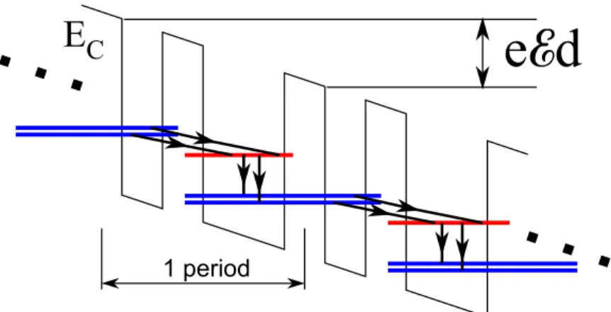
are periodic in energy and space: for any given eigenstate ψ(z) with energy E, there will be a whole set of corresponding states with eigenfunctions ψ(z −nd), and energies

E − eEnd, where E is is the applied electric field, d is the superlattice period, and n

is an integer. This is known as the Wannier-Stark ladder (see figure 2-2), and is the usual basis for QCL calculations. Transport occurs through scattering between these eigenstates, in the manner of the classical Boltzmann transport equation. The scat-tering rates themselves, however, are calculated quantum mechanically using Fermi’s golden rule (hence this approach is “semiclassical”).

There are, however, some theoretical difficulties with the Wannier-Stark states; al-though not so relevant to practical design, they are worth mentioning. The application of an electric field yields (up to some additive constant) the potential eΦ(z) = −eEz. A QCL superlattice is typically hundreds of periods long, making it effectively

(26)

infi-Figure 2-2: Schematic of Wannier-Stark Hopping conduction. Both the superlat-tice potential and the electric field are diagonalized, and transport occurs entirely through scattering between eigenstates. Equivalent WS states in adjacent periods are separated in energy by eEd.

nite in length. This results in a potential that extends essentially from −∞ to ∞ in energy, and consequently there are no bound states in the superlattice. In fact, the spectrum of the biased superlattice is mathematically proven to be continuous [30], even for arbitrarily small biases. On the other hand, the spectrum of an unbiased superlattice clearly has bound states, the experimental gain spectra of QCLs clearly shows discrete structure, and experimental absorption studies in other superlattice structures also support the existence of the Wannier-Stark ladder.

The resolution to this apparent paradox is that lasing in QCLs occurs between

resonant eigenstates that possess a discrete spectrum embedded inside a continuous

spectrum. One way to think about these resonant Wannier-Stark states is that they are the bound states of the unbiased superlattice, but the applied field induces them to possess a finite lifetime. This reflects that in the presence of a field, electrons possess a finite probability of leaking out of the quantum wells over time. As the field approaches zero, the escape rate approaches zero, or equivalently, the lifetime goes to infinity.

But the wavefunctions of the Wannier-Stark states are proven to have exponen-tially divergent tails at infinity, and hence are not unnormalizable in the usual sense (hψ|ψi = 1). This reflects that in the absence of scattering, electrons in a resonant state will eventually leak out, and then accelerate indefinitely [31]. Fermi’s golden

(27)

rule cannot be used with such pathological wavefunctions. Here, QCL design takes a refreshingly straightforward approach: for want of a better solution, the issue of unbounded wavefunctions is simply ignored. One or two modules of the superlattice are modeled as a closed system with Dirichlet boundary conditions (F (z) = 0 at simulation boundaries), and the resulting wavefunctions are normalized over the one or two module lengths. The resulting wavefunctions are well behaved, and Fermi’s golden rule applies.

There is no mathematically rigorous justification for this artificial approach to boundary conditions. Physically, however, the heavy scattering in semiconductor systems would prevent the indefinite acceleration corresponding to the unnormaliz-able tail of the Wannier-Stark states. The states of interest are quite often located energetically far below adjacent quantum barriers, such that one would expect the resonant lifetime to be long in comparison to scattering induced lifetimes. In this situation, the expectation that the electrons should be localized to within one or two modules is reasonable. However, the resonant lifetimes grow shorter at high applied fields, and the lifetime associated with “over-barrier” escaping electrons may possibly become significant even in comparison to scattering mechanisms.

Perhaps the strongest endorsement of this method, however, is purely empirical: practically all QCLs are designed using this approach, and the success of all these devices attest to the validity of this method, even though its theoretical foundations may not be solid.

Analytical QCL rate equation model

As an example of a rate equation approach, QCLs are often described by a restricted rate equation model examining only the upper and lower laser subbands coupled to the optical field in the device. Although this model attains reasonable quantitative agreement with mid-IR devices, it is insufficient for THz devices. Nevertheless, it deserves a brief overview here on account of its ubiquity in the literature, and also because it has some utility in the qualitative description of THz QCLs.

(28)

whose modes have uniform photon density (unachievable in practice of course, but consideration of the detailed modal information garners no additional insight). Let the upper and lower laser subband populations in the total device volume be denoted as n3 and n2 respectively (the designation “1” is normally reserved for the injector

subband; see chapter 3). Let there be a single lasing mode of negligible spectral width, modal volume Vph and total photon number nph. Then the rate equations for

n3, n2 and nph are dn3 dt = ηINm e − n3 τsp − n3− n2 τ0 sp µ nph Vph · V Nm ¶ − n3 τ3 dn2 dt = (1 − η)INm e + n3 τsp +n3 − n2 τ0 sp µ nph Vph · V Nm ¶ + n3 τ32 − n2 τ2 dnph dt = n3 τ0 sp + n3− n2 τ0 sp µ nph Vph · V Nm ¶ −nph τph (2.7)

The other symbols above are defined as follows:

• I is the device current. It is taken to be a model parameter.

• 0 < η < 1 is the injection efficiency into the upper level. It is taken to be a

model parameter.

• τsp is the total spontaneous emission rate, and τsp0 is the spontaneous emission

rate into the lasing mode.

• τ32 is the scattering lifetime of non-radiative processes from the upper to lower

subband.

• τ3 is the scattering lifetime of other upper level non-radiative processes.

• τ2 is the scattering lifetime of lower level non-radiative processes.

• τph is the photon lifetime in the optical cavity.

The term ³ nph Vph · V Nm ´

reflects that stimulated emission is proportional to the number of photons in each module, rather than the total number of photons. One may

(29)

abbreviate V /Vph as Γ, the confinement factor, which measures the fraction of the

optical mode overlapping with the active region.

In steady state, one sets all time derivatives in equations (2.7) to zero, and solves for the electron and photon populations. Above threshold, one must be careful to solve the equations with the amount of population inversion n3−n2 held constant. Of

particular interest is the degree of subthreshold population inversion, as this deter-mines whether there will be positive gain for lasing. Subthreshold radiative lifetimes are typically orders of magnitude higher than non-radiative lifetimes, so one may neglect all radiative terms. The result is that

∆n = n3− n2 = INm e · ητ3 µ 1 − τ2 τ32 ¶ − (1 − η)τ2 ¸ (2.8)

Let η ∼ 1 (this is not necessarily—or even likely to be— true, but is done for simplicity due to the difficulty of determining η from experiment or calculation). One finds that

∆n ∝ τ3 µ 1 − τ2 τ32 ¶ (2.9)

This simple rate equation model can be developed much further; the reader is referred to [32] for more elaborate treatments. However, due to the model’s limited applicability to THz devices, this section stops here.

2.2.3 Density matrix transport: the Kazarinov-Suris model

As a Boltzmann transport equation-like model, the Wannier-Stark hopping model de-scribed in section 2.2.2 admits a simple physical description and appeals to intuition. Current conduction occurs between the Wannier-Stark eigenstates having different average positions, enabling an electron to hop down the superlattice. However, fur-ther examination reveals a number of contradictions.

From a conceptual viewpoint, whereas Wannier-Stark hopping describes current as being driven by scattering, the miniband conduction model describes current as caused by coherence. In the miniband conduction model of transport, scattering in-duces transitions to different kz states, possibly in different minibands, but does not

(30)

change the average position of the electrons. Instead, the field-induced coherent evo-lution of the Wannier-Bloch states carries the current, and scattering is only relevant insofar as it interrupts the evolution.

From a empirical viewpoint, Callebaut has shown that the Wannier-Stark hopping model predicts unphysical behavior for current densities [33]. This is best explained by an example. Figure 2-3a depicts a two-well superlattice biased such that two single well states align in energy as indicated. When this resonance1 _or

anticross-ing occurs, diagonalization to calculate the Wannier-Stark states yields a delocalized

bonding/anti-bonding pair separated by an anticrossing gap, ∆. In the Wannier-Stark hopping model, transport occurs through scattering from this pair into subsequent modules. Although increasing the barrier thickness decreases the size of the anti-crossing gap, the wavefunctions are nearly unchanged, resulting in a current density essentially independent of barrier width. Experimentally, increasing the barrier thick-ness does decrease current density, a result consistent with physical intuition.

(a) (b)

Figure 2-3: (a) Extended wavefunctions used in Wannier-Stark hopping. (b) Localized wavefunctions coupled through a barrier used in the Kazarinov-Suris model. The gap between the extended states is ∆ = EA− ES ≈ 2U

The unphysical behavior of the Wannier-Stark hopping model is due to the neglect of coherent transport. To account for coherent effects, Kazarinov and Suris proposed a phenomenological density matrix model based on localized states (such as single well states2_{). Consider the same two-well superlattice in figure 2-3b. This time, the}

1_{Not to be confused with the “resonant eigenstates” discussed in section 2.2.2; those are}

eigen-states with finite lifetime even in the absence of scattering.

(31)

two states in resonance are modeled as a dissipative two-level system coupled through an interaction potential U. In matrix form, the Hamiltonian is

H =   E1 −U −U E2   _(2.10)

Diagonalizing H yields bonding and anti-bonding Wannier-Stark levels as before, with the coupling U responsible for the anticrossing gap at resonance (E1 = E2). The

density matrix evolves according to

i~d

dtρ = [H, ρ] + i~Γ(ρ) (2.11)

where the commutator [H, ρ] describes coherent evolution and Γ is the dissipation super-operator describing coupling to the environment (in this case, other superlattice states). Γ is approximated using a phenomenological relaxation time expression of the form Γ(ρ) =   ρ22 τ − ρ12 τ|| −ρ21 τ|| − ρ22 τ   _(2.12)

In this picture, transport occurs via two mechanisms. A particle initially localized in state 1 in the left well will resonantly tunnel into state 2, and back again, much like the Rabi oscillations of an optical two-level system; these oscillations are interrupted (damped) by the scattering of electrons from state 2 into state 1 of a subsequent superlattice period, with some time constant τ . In addition, there may be processes that do not change populations (the diagonal elements ρ11 and ρ22), but nonetheless

scramble the coherence of the tunneling process; the overall phase-breaking time τ||

combines the effects of these “pure” dephasing processes with the phase-breaking due to population changing scattering. Let the total electron population be N, such that

ρ11+ ρ22 = N. Solving equation (2.11) for steady state yields the Kazarinov-Suris

discussion ignores. A more appropriate choice might be, say, the Wannier function basis. The crucial point is that the basis is localized.

(32)

expression for the current through the barrier, J = eNρ22 τ = eN 2Ω2_τ || 4Ω2_{τ τ} ||+ ω212 τ||2+ 1 (2.13)

where Ω = U/~ and ω21 = (E2− E1)/~.

Consider the case of resonance (ω21 = 0). For strongly interacting states (thin

barrier), |Ω| À 1/√τ τ||. Electrons in this regime oscillate freely between states 1 and

2 with only light damping due to scattering effects (oscillations are underdamped). This case yields

J ≈ eN

2τ (2.14)

This expression is indeed independent of the interaction Ω between the two states and the phase-breaking time τ||. Transport is determined essentially by the scattering

time in this regime, so one expects the Wannier-Stark hopping model to be valid. In contrast, for weakly interacting states (thick barrier), |Ω| ¿ 1/√τ τ||. Electrons in

this regime scatter rapidly but tunnel slowly (oscillations are overdamped). This case yields

J ≈ 2eNΩ2_τ

|| (2.15)

Here one finds that current density is strongly dependent on the interaction between the two states and is sensitive to phase-breaking processes. This recovers the exper-imental result that current density does depend on the barrier width, as the barrier width factors into both Ω and τ||.

Note that the relaxation time approximation for Γ does not recover sensible results if the delocalized Wannier-Stark states are used as the basis. Although physical results should in principle be independent of the quantum basis, equation (2.12) for Γ is approximate, and our choice of basis affects the quality of the approximation. This can be illustrated by an example. At resonance (E1 = E2), diagonalizing equation

(2.10) yields

(33)

where HD =   E − U 0 0 E + U   =   ES 0 0 EA   , S = √1 2   1 1 1 −1   _(2.17)

The density matrix equation of motion (2.11) can be changed to the eigenbasis by multiplying both sides from the left by S† _{and from the right by S (in this particular}

example S = S†_{). The result is}

i~d dtρD = [HD, ρD] + i~ΓD(ρD) (2.18) where ρD = S†ρS =   ρSS ρSA ρAS ρAA   =   12(ρ11+ ρ12+ ρ21+ ρ22) 12(ρ11− ρ12+ ρ21− ρ22) 1 2(ρ11+ ρ12− ρ21− ρ22) 1 2(ρ11− ρ12− ρ21+ ρ22)   _(2.19) ρ = SρDS†=   ρ11 ρ12 ρ21 ρ22   =   12(ρSS+ ρAS + ρSA+ ρAA) 12(ρSS − ρAS + ρSA− ρAA) 1 2(ρSS+ ρAS− ρSA− ρAA) 1 2(ρSS − ρAS − ρSA+ ρAA)   _(2.20) and ΓD = S†ΓS (2.21) =   −2τ1||(ρ21+ ρ12) ρ22 τ − 2τ1||(ρ21− ρ12) ρ22 τ + 1 2τ||(ρ21− ρ12) 1 2τ|| (ρ21+ ρ12)   =         − 1 2τ||(ρSS − ρAA) 1 2τ (ρSS− ρAS − ρSA+ ρAA) − 1 2τ||(ρAS − ρSA) 1 2τ (ρSS− ρAS − ρSA+ ρAA) + 1 2τ||(ρAS − ρSA) 1 2τ||(ρSS − ρAA)        

(34)

The on-diagonal scattering has the expected form of a rate equation involving the populations, but the off-diagonals do not evolve through a simple relaxation of the form −ρAS/τD||.

Use of the Wannier-Stark basis leads to the erroneous conclusion that coherence plays no role in QCL transport. Unfortunately, Iotti and Rossi in their 2001 paper [34] introducing the use of ensemble Monte Carlo methods for QCL transport appears to have done exactly this: they employed a density matrix model in the Wannier-Stark basis with a scattering superoperator analogous in form to equation (2.12), with rates calculated using Fermi’s golden rule. Perhaps this is the reason why they came to the conclusion that a QCL’s transport is essentially incoherent. Callebaut modified the Monte Carlo density matrix technique to employ a tight-binding basis [35], and in doing so recovered the importance of coherence to transport. Weber et al. have also studied QCLs using a first principles density matrix formalism in the Wannier-Stark basis, concluding that coherence is crucial to transport [36]. The importance of coherence in QCL transport has also been affirmed in studies using the methods of NEGF [26, 37].

Quantitative application of the Kazarinov-Suris model is difficult because of large uncertainty in τ and τ||, and because often more than two states are of interest.

However, it highlights the key role of the anticrossing gap ∆ of delocalized Wannier-Stark states. This is because the interaction between the corresponding localized states can be estimated by U ≈ ∆/2, and hence ∆ is a key metric of resonant tunneling through thick barriers, where Wannier-Stark hopping is invalid. Chapter 3 considers in detail the injection anticrossing and the collection anticrossing.

2.3 Numerical Determination of Eigenfunctions

Equation (2.5) admits tractable analytical solutions only for a few simple potentials, such as the prototypical unbiased, single quantum well. In general, a numerical solution is faster and more fruitful. This section covers two common methods, and a useful, but lesser known third.

(35)

2.3.1 Finite difference method

The finite difference method approximates the differential equation to be solved by its values on a mesh of uniformly spaced points. Let the computational domain be of length L, meshed with N points spaced by δz = L/(N − 1), and assume Dirichlet boundary conditions. A 2nd order finite difference approximation of the envelope function derivative is

d

dzF (z) ≈

F (z + δz) − F (z − δz)

2δz (2.22)

Interestingly, if F is a vector whose entries are the values of the envelope function at the grid points (F [i] = F (i × δz)), then equation (2.22) defines a linear matrix algebra transformation for F . That is, if G is the vector representing the derivative of F (z), then F and G are related by

G = D₁F (2.23)

where D₁ is the infinite, tridiagonal matrix

D₁ = 1 2δz            . .. ... . .. 0 1 −1 0 1 −1 0 . .. . .. ...            (2.24)

Similarly, multiplication by a scalar function, such as the potential V (z), can be represented as multiplication of F by a diagonal matrix.

V =            . .. V [0] V [1] V [2] . ..            (2.25)

(36)

where, like the definition for F , V [i] = V (i × δz). Therefore, one may write down by inspection the finite difference approximation of equation (2.5) as a matrix eigenvalue problem. · −~ 2 2 D1M −1_D 1+ V ¸ F = EF (2.26)

where M−1 is the inverse effective mass matrix, which is diagonal like V . Finally, enforcing Dirichlet boundary conditions means F [0] = 0 and F [N] = 0; this enables truncation of the infinite dimensional matrix value problem of equation (2.26) into a (N − 2) × (N − 2) matrix value problem, which can be solved by any eigenvalue method of numerical linear algebra.

2.3.2 Shooting method

The finite difference methods above returns N −2 eigenstates, but one is normally only interested in a few of the lowest energy eigenstates. The numerical approximation worsens as the characteristic oscillations of the envelope function approaches the finite difference step size, so beyond some point in energy, the computed eigenstates degenerate into numerical garbage. This motivates the use of the shooting method, which directly computes the lowest energy eigenstates one at a time.

The shooting method for eigenfunction determination solves a 1D boundary value problem using the numerical methods of time-dependent ordinary differential equa-tions. A typical time-dependent problem starts at an initial condition at some time

t, and uses some approximation of the differential equation to determine the solution

at a later time t0 _{= t + δt. In this manner, the solution can be traced in time by steps}

of δt.3 _{In the shooting method, the same procedure is applied to a spatial coordinate.}

The solution at some boundary z1 is integrated forward by steps of δz until a second

boundary z2 is reached. However, in the shooting method, some of the boundary

con-3_{Although the section assumes constant δt, this is not necessary in general. Clever shooting}

method implementations may adjust δt in response to how quickly they perceive the solution to be changing at a given current point in time, optimizing the trade-off between resolution and solution speed.

(37)

ditions at z1 and the eigenvalues are left as adjustable parameters to fit the boundary

conditions at z2. This motivates the name “shooting method”: one targets (“shoots

at”) a boundary condition on the opposite side of the computational domain.

An example is helpful for clarification; the following shooting method is presented by Harrison for the solution of equation (2.5) [38]. One starts by deriving the following finite difference approximation of equation 2.5:

· −~2 2 d dz 1 m∗_(z) d dz + V (z) ¸ F (z) = EF (z) ⇒ −~ 2 2δz " 1 m∗_{(z + δz/2)} dF dz ¯ ¯ ¯ ¯ z+δz/2 − 1 m∗_{(z − δz/2)} dF dz ¯ ¯ ¯ ¯ z−δz/2 # + V (z) = EnFn(z) ⇒ −~ 2 2δz · 1 m∗_{(z + δz/2)} F (z + δz) − F (z) δz − 1 m∗_{(z − δz/2)} F (z) − F (z − δz) δz ¸ +V (z) = EnFn(z) ⇒ −~ 2 2(δz)2 · F (z + δz) − F (z) m∗_{(z + δz/2)} − F (z) − F (z − δz) m∗_{(z − δz/2)} ¸ + V (z) = EF (z) (2.27)

In the above, Harrison takes m∗_{(z ± δz/2) to be the average effective mass between}

two points, but another possible choice is to instead calculate the average inverse effective mass between two points; the difference is small unless the heterostructure has extremely mismatched effective masses. One may rewrite equation (2.27) to yield the solution for a subsequent point as function of the previous two points. This reads

F (z + δz) m∗_{(z + δz/2)} = · 2(δz)2 ~2 (V (z) − E) + 1 m∗_{(z + δz/2)} + 1 m∗_{(z − δz/2)} ¸ F (z) − F (z − δz) m∗_{(z − δz/2)} (2.28)

Using Dirichlet boundary conditions, the initial conditions at the left-hand side of the simulation boundary are that F (z = 0) = 0 and F (z = δz) is any non-zero value. The arbitrariness of F (z = δz) is because eigenfunctions are unique only up to a multiplicative constant, said constant being determined by wavefunction normalization requirements and itself determined only up to a complex phase factor.

(38)

Integrating over to z = L, one treats F (z = L) as a function of E, and scans E through some range of energies to find solutions satisfying F (z = L) = 0. A root-finding algorithm (for example, the secant method or Newton-Ralphson method) is used to refine the value of E when close to an eigenvalue.

Paul and Fouckhardt introduced a superior shooting method in [39]. In this alternate method, one defines

G(z) = 1 m∗_(z)

d

dzF (z) (2.29)

and specifies different, but coupled, shooting equations for F and G. This yields

G(z + δz) = G(z) + 2δz

~2 (V (z) − E)F (z)

F (z + δz) = F (z) + δz m∗_(z)G(z) _(2.30)

These equations are simpler to compute than equation (2.28), and reference [39] also shows them to be more numerically stable.

2.3.3 Spectral element method

Before discussing the spectral element method, one must first understand the more specific technique of spectral methods. This thesis could not possibly do justice to this rich subject area, so the introduction here is necessarily qualitative. The interested reader is referred to Boyd’s excellent textbook [40].

Spectral methods take a philosophically different approach to numerical solution from the finite difference approximation on which both the finite difference method and the shooting method is based. Spectral methods pick some basis of orthogonal functions, and assume that the solution of a problem can be expanded in this basis. One then attempts to find the expansion coefficients of the series. Whereas accuracy of a solution is determined by the step size δz in the finite difference approximation, it is determined by the number of terms retained in the expansion in spectral methods. Qualitatively, one could say that finite difference method finds exact solutions to

(39)

an approximation of the problem, whereas spectral methods try to find approximate

solutions to the exact problem. A well-chosen basis results in exponentially fast

convergence. Since finite difference methods converge only algebraically, spectral element methods practically always achieve better accuracy for a given number of points—sometimes dramatically so.

Like in quantum mechanics, the choice of basis depends somewhat on the problem at hand, but is also largely a matter of taste. Surprisingly, there exist a class of orthogonal functions whose expansion coefficients are equal to the value of the solution at certain points (nodes), the Lagrange interpolation polynomials. It turns out that if these points are chosen to be zeros or extrema of another basis set (usually the Chebyshev polynomials of the first kind), the Lagrange interpolation polynomials will inherit the same convergence properties. Ironically, the practical implication of using the Lagrange interpolation polynomials as a spectral basis is that the spectral method is merely solving for the values of the solution on a non-uniform grid. Phrased as such, this pseudospectral method does not sound so different from the finite difference method, despite the philosophical differences explained previously.

A major difficulty with spectral methods, however, is that they lose their excel-lent convergence properties in the vicinity of discontinuities. A well-known example of this is Gibb’s phenomena seen in the Fourier expansion of piecewise continuous func-tions. Unfortunately, the envelope function problem for a heterostructure is riddled with discontinuities, both in the effective mass and in the potential. The solution, as first advocated by Patera [41], is to divide the computational domain into smooth sub-domains, or elements, each possessing its own series expansion, and then enforce boundary conditions between elements. A superlattice lends itself well to this ap-proach, as one can treat each layer as a separate element. This essentially combines spectral methods with the finite element method, resulting in the spectral element

method.

Unfortunately, the mathematics of the spectral element method are significantly more complicated to derive. The pseudospectral variant used in this thesis is based on the method reported in [42]. It uses the Gauss-Legendre-Lobatto (GLL) nodes, and

(40)

possesses the convergence properties of a direct expansion in Legendre polynomials. On the normalized interval [-1,1], the N GLL nodes are the extrema of the (N − 2)th Legendre polynomial and the two end-points ±1. Denoting these as ζn, they can be

remapped as necessary onto any other linear interval [a, b] through the transformation.

zn =

b + a

2 + ζn

b − a

2 (2.31)

Let the Lagrange interpolation polynomials be denoted bn(z). The derivation starts

by considering just a single element. First, the inner produce (integral) of both sides of equation (2.5) is taken against an arbitrary bm(z) (readers familiar with finite

element methods will recognize this as Galerkin’s method). This yields

−~ 2 2 Z C dz bm d dz 1 m∗ d dzF + Z C dzbmV F = E Z C dzbmF (2.32)

where C is the length of the element under consideration, and the argument depen-dences of the functions have been suppressed for clarity (eg. F really should be F (z)). The first term is expanded using integration by parts

Z C dz bm d dz 1 m∗ d dzF = · bm m∗ dF dz ¸ ∂C − Z C dz dbm dz 1 m∗ dF dz = δm0 · 1 m∗ dF dz ¸ z=z0 − δmN · 1 m∗ dF dz ¸ z=zN − Z C dz dbm dz 1 m∗ dF dz (2.33)

The last step above uses a property of the Lagrange interpolation polynomials that

bm(zn) = δmn, where zn is the nth GLL node. Next, the series expansion

F (z) =

N

X

n=1

(41)

where Fn = F (zn), is inserted into equations (2.32) and (2.33), yielding −δm0 · ~2 2m∗ dF dz ¸ z=z0 + δmN · ~2 2m∗ dF dz ¸ z=zN +~ 2 2 N X n=1 ·Z C dz dbm dz 1 m∗ dbn dz ¸ Fn + N X n=1 ·Z C dz V bmbn ¸ Fn= E N X n=1 ·Z C dzbmbn ¸ Fn (2.35)

In principle, the integrals above can be integrated analytically, but numerical integra-tion in this case is much simpler. Conveniently, the GLL nodes are the same nodes at which a function needs to be evaluated in order to perform Gaussian quadrature. Gaussian quadrature of order N approximates a normalized integral in [-1,1] as

Z ₁ −1 f (ζ)dζ ≈ N X p=1 wpf (ζp) (2.36)

and for an arbitrary interval [a, b], Z _b a f (z)dz ≈ N X n=1 (b − a)wp 2 f (zp) = N X p=1 Wpfp. (2.37)

(The integration weights wp are given in [40]). Applying Gaussian quadrature and

after doing some algebra, equation (2.35) becomes

−δm0 · ~2 2m∗ dF dz ¸ z=z0 + δmN · ~2 2m∗ dF dz ¸ z=zN +~ 2 2 N X n=1 " N X p=1 dbm(zp) dz Wp m∗ p dbn(zp) dz # Fn +VmWmFm = EWmFm (2.38)

Equation (2.38) defines a set of N equations in the element of consideration; essen-tially, it leaves one with a mini-matrix problem for each element, and it remains to combine them. Consider now two adjacent regions A and B, with NA and NB

points respectively. At the boundary between A and B, boundary conditions (2.6) imply that FA(zN,A) = FB(z0,B), motivating one to add together the last equation

of A and the first equation of B. But the boundary terms h ~2 2m∗dF_dzA i z=zN,A=z0,B and

(42)

h

~2

2m∗dF_dzB

i

z=zN,A=z0,B

are equal, and so cancel. The essential point is that all the in-ternal boundary terms between elements cancel out when the sets of equations for different elements are combined. Furthermore, Dirichlet boundary conditions enables one to discard the external boundary terms at the edges of the computational domain. Ultimately, one finds that equation (2.5) can be approximated by the generalized, lin-ear, matrix eigenvalue problem

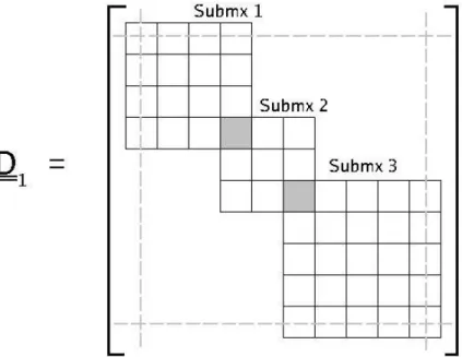
· ~2 2D T 1M −1_{W D} 1+ V W ¸ F = A F = EW F (2.39) It is difficult to discuss the structure of the matrices without a specific example, so consider a computational domain partitioned into 3 elements with 4, 3 and 5 nodes, respectively. Consider D₁: each element will contribute an elemental sub-matrix and these will be assembled into D₁ by “overlapping and adding together at the corners.” For example, the elemental sub-matrix of the first element has elements defined by

h D(1) 1 i mn = db(1)n (zm) dz (2.40)

where b(1)n are the Legendre interpolation polynomials for region 1 (formulae for the

pseudospectral differentiation matrices are given in [40, 43]). D₁ is schematically shown in 2-4. The inverse effective mass matrix M−1 _{and the matrix of Gaussian}

quadrature weights W are similarly assembled from the inverse masses and quadrature weights evaluated at the nodes in each element. (Conveniently, these last two matrices are diagonal.)

The problem specification is complete at this point, but Cheng et al. [42] introduce a final numerical method to turn generalized eigenvalue problem (2.39) into a regular eigenvalue problem by manipulating equation (2.39) into

A F = EW F ⇒ W−1/2A ³ W−1/2W1/2 ´ F = EW1/2 F ⇒ A0F0 = EF0 (2.41)

(43)

Figure 2-4: Schematic of pseudospectral differentiation matrix for the spectral element method, for a hypothetical computational domain partitioned into three elements having 4, 3, and 5 nodes, respectively. The differentiation matrices for each region are assembled into D₁ by overlapping and adding together boundary entries (indicated in grey). Dirichlet boundary conditions enable one to strike out the first and last rows and columns (dotted lines).

Where A0 = W−1/2A W−1/2 and F0 = W1/2F . As with the finite difference method,

this eigenvalue problem can now be solved using any eigensolver.

2.3.4 Comparison of methods

Both the finite difference method and spectral element method require linear algebra eigensolvers; the most basic and reliable of these is the QR method, and its cousin for generalized eigenvalue problems, the QZ method [40]. Unfortunately, the QR/QZ methods can be numerically expensive, with costs scaling as O(N3_{) where N is the}

matrix size or number of nodes (these being approximately equal). In contrast, as-suming some average number of root-finding iterations for each eigenfunction, the shooting method scales as O(NM ), where M is the number of points to scan in energy (assuming linear scan). M will depend on the number of eigenfunctions re-quested and the nature of the particular potential. For example, one might expect that M would scale as the square of the number of requested eigenfunctions in an

(44)

infinite quantum well. But in general, M will be modest compared to N2_{. This}

favor-able scaling makes the shooting method potentially the fastest of the three methods, achieving finite difference accuracy at a fraction of the cost of eigensolver routines when N becomes large.

Unfortunately, the shooting method’s speed comes at the cost of stability. From quantum mechanics, Schr¨odinger’s equation in regions where the potential energy surpasses the particle energy leads to exponentially growing or decaying waves with imaginary wavevector. The exponentially divergent solutions frequently lead to nu-merical overflow when one integrates from a well into a thick barrier, causing the shooting method to crash (for this reason it is also necessary to shoot in the direction of decreasing electric potential energy). Although the shooting method usually does converges, it is the author’s experience that there is no easy way of predicting when it does not, nor of salvaging broken problems. In contrast, both the finite difference method and spectral element method are very robust.

The advantage of spectral elements over finite differences is that the exponential accuracy of the former enables one to use far fewer solution nodes. This greatly speeds up the QR algorithm. As numerical methods are not the focus of this thesis, this section makes no attempt at a controlled study comparing finite differences and spectral elements (see [42] for such a study), but nevertheless, a semi-quantitative example is illuminating.

This thesis uses a custom spectral element code developed in MATLAB 7.0. The tool of choice for the last three generations of graduate students working on the THz QCL project at MIT is the SEQUAL 2.1 finite difference code developed in the 1980s at Purdue University [44] (the order of the finite difference approximation is unknown). The spectral element code of this thesis normally uses 1 node every 2 monolayers, whereas the SEQUAL 2.1 convention is to use 2 nodes per monolayer. Ignoring prefactors to the computational costs, the QR algorithm scaling suggests a 64-fold reduction in computation time. To test this, table 2.1 compares the perfor-mance of this thesis’s code and SEQUAL 2.1 in computing the two-module eigenstates of QCL design OWI185E-M1 (see section 4.2.3). It is difficult to get both programs to

(45)

SEM SEQUAL 2.1 0.5pts 1.0pts Rel. err 2.0pts 4.0pts Rel.err

Eij /ML /ML (%) /ML /ML (%)

(meV) (meV) (meV) (meV)

E32 37.80 37.80 0.466e-4 37.90 37.94 -0.0933 E43 5.138 5.138 5.765e-4 5.127 5.129 -0.0544 E54 5.137 5.137 -2.628e-4 5.162 5.164 -0.0341 E65 13.75 13.75 -0.327e-4 13.95 13.98 -0.2419 E76 3.212 3.212 11.65e-4 3.182 3.176 0.2009 E87 35.57 35.57 -1.435e-4 35.72 35.76 -0.1157 E98 4.809 4.809 5.868e-4 4.802 4.8 0.03521 E10,9 2.737 2.737 -15.10e-4 2.257 2.238 0.8526 E11,10 2.621 2.621 13.48e-4 3.133 3.16 -0.8472 E12,11 9.425 9.425 -3.812e-4 9.138 9.095 0.4791 E13,12 7.192 7.192 13.23e-4 7.627 7.685 -0.7600 E14,13 23.78 23.78 -4.075e-4 23.33 23.28 0.1980 E15,14 13.72 13.72 0.010e-04 13.81 13.83 -0.1357 Time(s) 0.083 0.600 2.75 23.0

Table 2.1: Performance comparison of custom spectral element method (SEM) im-plemented in MATLAB 7.0 versus SEQUAL 2.1. Reported are the energy differences between adjacent eigenstates at different resolutions. The relative error is specified relative to the higher resolution calculation for both methods.

agree on exactly the same eigenvalues (due to slight differences in parameters, round-ing, etc.), so table 2.1 compares relative accuracy for each program: for each method, the eigenvalue problem is solved, and then the calculation is repeated with twice the resolution. The results from the differing resolutions are compared to see how well converged the solution is. Although the results of table 2.1 are not well controlled (for example, SEQUAL must spend spend additional time writing results to hard drive, making the contest stacked against it), the spectral element method clearly outper-forms SEQUAL 2.1 in both speed and relative accuracy. The actual speed increases are ∼33 between the two low resolution computations, and ∼38 between the two high resolution calculations. The reasons for the factor of ∼2 discrepancy from 64 are not known.

A few minor points in closing: there is also a risk of the shooting method acciden-tally skipping over closely spaced eigenvalues, but it is the author’s experience that the aforementioned stability problems are a more severe issue. On the other hand,

(46)

the shooting method can account for non-parabolicity using a energy-dependent effec-tive mass at no additional cost. In contrast, equation 2.5 with an energy dependent effective mass cannot be cast into a linear eigenvalue problem, so the finite difference method and spectral element method both require iterative solutions where none were necessary before. However, non-parabolicity is generally not considered in this thesis. Finally, the spectral element method’s non-uniform grid accommodates layers of ar-bitrary thickness, not just multiples of the step-size δz as in the finite difference and shooting methods.

2.4 Non-radiative Scattering Mechanisms

Having established the eigenstates of the biased superlattice, this section considers the scattering mechanisms which drive transport. All scattering rates here are calculated using Fermi’s golden rule.4 _{The treatment here is standard. The derivations below are}

also covered in Smet [45], Callebaut [33], Harrison [38], and other excellent sources. The eigenstates of the superlattice are uniquely identified by a subband number and an in-plane momentum.5 _{In this context, Fermi’s golden rule for scattering}

from a state i, ki (subband i with momentum ki, energy Ei(ki) = Ei + ~ 2_k2

i

2m∗, and

envelope function Fi(z)eiki·r√_A ) to a state f, kf (subband f with momentum kf, energy

Ef(kf) = Ef+ ~2_k2 f 2m∗, envelope function Ff(z)e ikf ·r √

A ) due to a time-harmonic perturbing

potential H0_{(t) = H}0_e±i∆E/~t _reads

W¡i, ki → f, kf ¢ = 2π ~ ¯ ¯_{f, k}_f _{| H}0 _{| i, k} i ®¯_¯2 δ¡Ef(kf) − Ei(ki) ± ∆E ¢ (2.42)

where ∆E is the energy absorbed from or released to an intermediate entity such as a phonon or photon, and δ represents the Dirac delta function; its presence reflects that energy must be conserved over long time scales.

A note on the calculation of matrix elements in Fermi’s Golden Rule: given two

4_{First formulated by Dirac, Fermi being its titular spokesman notwithstanding.}

5_{Spin is ignored here because spin-up and spin-down are degenerate in the absence of an applied}

(47)

perturbations H0

1 and H20, one normally proceeds to calculate

¯ ¯_{f, k}_f _{| H}0 1 | i, ki ®¯_¯₂ and ¯ ¯_{f, k}_f _{| H}0 2 | i, ki ®¯_¯2 instead of ¯¯f, kf | H10 + H20 | i, ki ®¯_¯2

. While the latter matrix element seems more mathematically well motivated, the cross-terms between H0

1 and

H0

2 complicates analysis. The standard approach is much more convenient because,

by neglecting these cross-terms (correlations), scattering rates for each mechanism can be calculated independently and directly added together. The neglect of cross-terms is physically equivalent to assuming uncorrelated scattering mechanisms, which is an assumption somewhat justifiable given that Fermi’s golden rule is accurate only in reflecting mean behavior of weak scattering over long time scales. But ultimately, the real motivation is probably mathematical convenience: given that any golden rule analysis is only approximate anyway, the extra rigor likely nets little advantage over the simpler approach.

2.4.1 Scattering by longitudinal optical phonons

Scattering by longitudinal optical (LO) phonons is the most important scattering mechanism in QCL transport, since it yields sub-picosecond scattering times in polar semiconductors such as GaAs/AlGaAs. This is a two-edged sword. The phonon depopulation QCL designs studied in this thesis (see chapter 3) use this ultrafast LO phonon scattering for depopulating the lower laser subband to create population inversion, but it is also hypothesized to be a major source of non-radiative scattering of electrons from the upper laser subband (recall section 1.1).

The section treats scattering of subband electrons from a thermalized gas of dis-persionless, bulk GaAs LO phonon. This treatment is approximate, since the differing mechanical properties of quantum wells and quantum barriers will induce quantiza-tion in the phonon spectrum as well. However, studies by Williams [46] and Gao [47] suggest that calculations based on detailed phonon spectra make little difference to overall scattering rates. Because QCLs are mostly GaAs (the barriers are typically only 15%-30% aluminum), even in more detailed calculations scattering tends to be dominated by GaAs-like phonon modes [46]. Moreover, screening and renormalization

Characterization and analysis of highly diagonal Terahertz Quantum Cascade Lasers

Characterization and Analysis of Highly Diagonal

Terahertz Quantum Cascade Lasers

by

Chun Wang Ivan Chan

Submitted to the Department of Electrical Engineering and Computer

Science

in partial fulfillment of the requirements for the degree of

Master of Science in Electrical Engineering

at the

MASSACHUSETTS INSTITUTE OF TECHNOLOGY

September 2010

c

° Massachusetts Institute of Technology 2010. All rights reserved.

Author . . . .

Department of Electrical Engineering and Computer Science

August 25, 2010

Certified by . . . .

Qing Hu

Professor

Thesis Supervisor

Accepted by . . . .

Terry P. Orlando

Chairman, Department Committee on Graduate Theses

Characterization and Analysis of Highly Diagonal Terahertz

Quantum Cascade Lasers

by

Chun Wang Ivan Chan

Abstract

Acknowledgments

Contents

List of Figures

List of Tables

Chapter 1

Introduction

1.1

Quantum Cascade Lasers

1.2

THz QCL Temperature Performance

1.3

Thesis Overview

Chapter 2

The Theory of Quantum Cascade

Laser Operation

2.1

The Envelope Function Approximation (EFA)

for Superlattices

2.2

Approaches to Transport: on the Choice of

Basis

2.2.1

Miniband conduction

2.2.2

Wannier-Stark hopping: the semiclassical rate

equa-tions

2.2.3

Density matrix transport: the Kazarinov-Suris model

2.3

Numerical Determination of Eigenfunctions

2.3.1

Finite difference method

2.3.2

Shooting method

2.3.3

Spectral element method

2.3.4

Comparison of methods

2.4

Non-radiative Scattering Mechanisms

2.4.1

Scattering by longitudinal optical phonons