FROM SATELLITE OBSERVATIONS by
AFFONSO DA SILVEIRA MASCARENHAS, JR.
B.S. Universidade de Sao Paulo (Brasil) (1967)
M.Sc. Instituto de Pesquisas Espacias (Brasil) (1975)
SUBMITTED IN PARTIAL FULFILLMENT OF THE REQUIREMENTS FOR THE
DEGREE OF MASTER OF SCIENCE
at the
MASSACHUSETTS INSTITUTE OF TECHNOLOGY
February, 1979
Affonso da Silveira Mascarenhas, Jr.. 1979
Signature of Author... ...
Department of Meteorology, February, 1979 Certified by...
Thesis Supervisor Accepted by...g.... ...
Chairman, Depargi ntal Committee on Graduate Students
MT
L1S
ACKNOWLEDGEMENTS. - . . . . . .. . . . - - - -. 1. INTRODUCTION. . .. -. * -1.1 The Scope of the Problem. . . . . . . . .. - . . .. . -. 1.2 Basic Equations and Assumptions. . . . . .. . . -. .. .. .
1.2.1 The Boussinesq Approximations. .. . . . . - -. .. . . 1.2.2 The Brunt-Vaisala Frequency. . . . . . . - - -. . .. . 1.2.3 The Equation for Internal Waves. . . . . . . . . . . .. 2. THE MODELS, THEIR SOLUTIONS AND DISCUSSION. . . . .. . .. . . 2.1 The Two-Layer Model . . .. . . - - - .. -2.2 The Three-Layer Model. . .. . - - - -. .. - - - - -. -. . 3. DATA AND MEASUREMENTS . . .. . - -. - - - -. 3.1 What the Internal Gravity Waves on the Continental Shelf
Look Like . .. . . - . . - - - -. 3.2 The Images, Climatological and Ground Truth Data - .. . -. . 3.3 Preliminary Analyses of the Measurements . . . - - - -. . 4. THE MIXED LAYER DEPTH IN THE OCEANS . . . . . . - - - -. . . . 4.1 The Establishing Factors of the Depth of Mixed-Layer . .. .. 4.2 Estimation of the Mixed-Layer Depth. . .. . - - - . . 4.2.1 From Two-Layer Model. . . . . . - - - -. 4.2.2 Comparison with Ground Truth Data - .. - - - -. . . . 5. THE AMOUNT OF HEAT STORED IN THE UPPER LAYER. . . .. . . . . 5.1 The Role of the Stored Heat. . . . . . -. - - - -. 5.2 Heat Stored Calculations from In-Situ Measurements . . .. . . 5.3 Heat Stored Calculations from Satellite Images . . . . - -. . 5.3.1 Based on Two-Layer Models . . . . . - - - -. 6. RESULTS . . . . . . . ..-.-.-.-.-.-.-.-.--.-.-.-.-.-. *.-.-. 6.1 The Accuracy and Dispersion of Q and
h..-.-.-.-.-.-.-.-.-.-.-6.2 Discussion of the Results for a Two-Layer Model. . . .. -. . 6.2.1 Mixed Layer Depth . . . - - - . - - - -. 6.2.2 Amount of Heat Stored . . . -. -. .. . - - - - -. 6.3 Additional Comments . . -7. CONCLUSIONS AND RECOMMENDATIONS . . . . . - - - -. REFERENCES. . . . . . - . - - - -. '
-CHARACTERISTICS OF UPPER HEATED OCEANIC LAYER FROM SATELLITE OBSERVATIONS
by
AFFONSO DA SILVEIRA MASCARENHAS, JR.
Submitted to the Department of Meteorology, February, 1979, in partial fulfillment of the requirements for the degree of Master of Science.
ABSTRACT
Velocity of propagation of internal wave packets over the New England American Continental shelf were computed from Landsat A/B
images taken in July and August of 1972, 1973, and 1974. A simple two-layer ocean model was used to compute from the velocity of propagation and climatological values of bottom density, the depth of the mixed layer and the amount of heat stored in the upper layer of the ocean. The comparison with in-situ observations showed a
good agreement for the amount of heat. Due to the internal wave noise in the hydrographic observations the calculated values for mixed layer depth differ from those computed from satellite data.
Charts of distribution of mixed layer depth and amount of heat stored based on 78 observations for the months of July and August are shown. In the Gulf of Maine heat stored values larger for July than August were found. A possible explanation for this anomaly is suggested in terms of air-sea interaction processes.
Thesis Supervisor: Erik Mollo-Christensen Title: Professor of Oceanography
I wish to thank Professor Erik Mollo-Christensen for the suggestion of the topic, his enormous amount of patience and faith in the author's abilities, and his guidance in all stages of the thesis.
Thanks are also extended to Dr. V. Worthington of Woods Hole Oceanographic Institution for furnishing most of the data, to Dr. G. Heimerdinger of NOAA for furnishing the new available data, to
Diana Spiegel for permitting me to use hours of computer time, to
Carlos Cardelino for the help with the programming problem, to Dr. Inez Fung for her valuable suggestions and help, to fellow classmates for the helpful discussions, to Virginia Mills for her excellent job of typing the manuscript and editing the Brazilian English, and finally, to the good friends on the 17th floor for their cherished friendship and incentive.
Special thanks are extended to my wife Terumi, my daughter Teozinha, and my son Jorge for their patience and understanding.
Financial support was provided by the Conselho Nacional de Desenvolvimento Cientifico e Technologico (CNPq) (Brazil) and by Universidade de Sao Paulo (Brazil).
1. INTRODUCTION
1.1 The Scope of the Problem
If one chooses not to classify aerial photography as Remote Sensing, the first attempt to extract information about the surface of the oceans
sensing remotely came about 25 years ago. The first occasion was when Stommel and Parson (1955), using an Airborne Radiation Thermometer, surveyed the Gulf Stream from an airplane. Broad and synoptic coverage are one of the advantages of this new technique and at the present state of the art we cannot classify Remote Sensing as an independent tool of research, but we have to admit that it is a powerful auxiliary tool.
One hears the argument that only surface observations can be made from airplanes or satellites, while the oceanographers are interested in vertical information as well. This work represents an attempt to correlate information available from satellites and oceanographic plat-forms as well as trying to infer a three-dimensional picture of oceanic phenomena. One prominent oceanographic feature that plays an important role in the dynamics of the continental shelf waters is the presence of internal wave packets.
As a subsurface feature the internal waves cannot be detected
directly by Remote Sensing, but their effects on the surface are visible. Apel and Charnell (1974) explain the internal waves sources and sinks admitting these waves as "daughter" waves generated for a few hours during the peak current velocity by the long-wavelength baroclinic tide occurring at the edges of the continental shelves and island arcs.
They then propagate with very low phase speeds, of ofder 0.25 to 0.5 m/sec, to be absorbed near the bottom where the wave breaks on the shelf.
explanations for why internal wave fields affect the surface of the ocean. The first one suggests that the velocity field of internal waves sweeps together surface oils and materials to formia slick in regions of surface water convergence, increasing the reflectivity of the surface
(Ewing, 1950, Shand, 1953). The second explanation is that capillary wave energy is focused in the convergence zones, enhancing the small-scale roughness and decreasing the surface reflectivity (Gargett and Hughes, 1972, Thompson and West, 1972). In either case, quasi-periodic
surface features will be produced under light wind conditions, and such effects are very often seen at sea. Under favorable conditions these features can be seen in satellite images as wave packets on the continen-tal shelf areas. The packets are apparently emitted once per tidal
period at the shelf edge (Apel et al., 1975). This assumption is sup-ported by the fact that the M2 component of the internal tide is found
to be dominant (Halpern, 1971, Barbee, 1975, Ratray, 1960). Figure 1-1 shows an schematic diagram of the internal wave propagation over the continental shelf and the associated surface slicks.
The eastern coast of the United States (from Cape Hatteras to Nova Scotia) provides favorable conditions for detection of internal wave packets on their continental shelves. The prevalence of internal wave signatures in that area during summer was recognized, and their dependence on the well-defined and relatively shallow thermocline was deduced from their-absence during winter months (Apel et al., 1974).
BREAKING
MIXED LAYER
30-60m
NINTERNAL
WAVES
-
-
-
--
--
..
THERMOCLINE
CONTINENTAL
-
-INCOMING
TIDE
SCHEMATIC DIAGRAM OF INTERNAL
WAVE PROPAGATION
Figure 1.1 - Schematic diagram of
over the continental
the internal wave propagation shelf (after, Apel 1974). SHErLF
internal gravity waves from which we know the velocity of propagation taken from the images. This information is enough to compute the depth of the mixed layer and the heat stored in the seasonal upper warm
layer of the ocean.
The heat stored in the upper ocean affects weather, both climatolo-gically and synoptically, and the mixing processes in the layer, driven by wind and thermal effects, also transport oxygen, nutrients and biota.
All these processes show therefore the importance of the knowledge of
the seasonal upper layer.
An extension for a three layer ocean, with the upper and lower
ones homogeneous and the middle layer with a linear variation thermocline is also made, and the results of the computation are discussed.
1.2 Basic Equations and Assumptions
The basic set of equations is: conservation of momentum, mass, and equation of state for sea water. The conservation of momentum can be written (see, for instance, Phillips, 1966)
N
xir=
-..
J
Vp. ~
(1.2.1)
where Vxv(9,+) denotes the velocity of the fluid at prescribed points in space-time as in an Eulerian description. The velocity compo-nents following x, y and z are respectively u, v, and w. -At is the rotation vector, or twice the earth's angular velocity. Its magnitude is
v4b
, is the gravitational potential, which contains the gravita-tional term (9 representing the apparent gravitational acceleration, or the true (central) gravitational acceleration modified by the small (centrifugal) contribution normal to the axis of the earth'srotation. The term VP represents the pressure gradient forces, and p is the density of sea water given as
/
/0
(-TSP)
(1.2.2)
The conservation of mass is expressed by
_ +V*(/-a) =c (1.2.3)
As in the Eulerian formulation, the total time derivative (derivative following the motion) is the sum of the time rate of change at a fixed point and a convective rate of change
(:Ppa
B~)=
0(1-2.1.1)
oZ
and if we subtract this equation from (1.2.1) we get
2 X 0 (1.2.1.2)
J t
where
j
Pis
In the ocean the difference between the actual state and the refer-ence state is the result primarily of surface heating or cooling, whose influence is distributed by the process of convection and mixing.
Surface water in regions of low salinity and high temperature has a 3
density as low as 1.02 gm/cm3. Water in the deepest trenches is subjected 3
to the highest pressures and has a density as high as 1.07 gm/cm So the maximum range is only about 5%!
Boussinesq in 1877 introduced an important approximation, namely; "The variations in the fluid density are neglected in so far as they influence the inertia terms, variations in the weight (or buoyancy) of the fluid may not be negligible."
So in (1.2.1.2) it is possible to approximate P by P.
But taking into account the fact that in the ocean the scale of vertical movements is much less than the scale height, an even greater
simplifi-cation can be done, also since the reference density Ps varies little from the constant mean value PO . So we can rewrite (1.2.1.2)
..
zto
)
(1.2.1.3)Using the fact that the mean value the buoyancy and pressure terms in
S
x\V
=-
P
P
0 is hydrostatic, we can modify(1.2.1.3) to get finally
P-t) (1.2.1.4)
where P now represents the difference between the actual and the hydrostatic pressure in an ocean at rest with constant density PO
Let us see now the effect of Boussinesq approximation in the conser-vation of mass equation (1.2.3). If P
=
PO we will not havestrati-fication at all. Since we want Boussinesq approximation as well as stratification, we say that our density is not constant, but varies a little around the mean value P0 . This statement can be written analytically as
0 W/P + ,F + 0 (1.2.1.5)
where-
p
)
is the added stratification and P is the variation in the density field due to internal waves. The expression (1.2.1.5)is called quasi-Boussinesq approximation. The new conservation of mass equation is
(1.2.1.6)
4.
The conditions for validity of Boussinesq approximation are:
a) The actual density distribution differs only slightly from the reference state;
b) The vertical scale of motion is small compared with the scale
height;
6C-
O (2oo km
) >>
H
-
0 ( 4 k
)
c) The Mach number of the flow is very small; for water at 15*C, c = 1470 m/sec, u = 5 cm/sec, M = 0.34x10~4,
so for the ocean all the requirements are fulfilled.
Expanding (1.2.2) about the basic state density /00 and neglecting the second order terms we get
p'= yi (-x T' kP'+ VS') (1.2.1.7)
where
(coefficient of thermal expansion) ;
(coefficient of isothermal compressibility);
(fractional increase in density per unit increase in salinity keeping T and P constant)
7
j0
A
If we substitute (1.2.1.7) in the right-hand side of (1.2.1.4), the vertical component of (1.2.1.4) has on the right-hand side the terms
For oceanic motions the vertical scale of variation H is of order 105 cm, so that the first term has magnitude Ip'I /H. The isothermal compressi-bility k has a magnitude of 4.5x10~1 in cgs units, so that the term gkp' has a magnitude I p
ll/Hs,
where Hs = 1/gk is the scale height for sea water. Its value is 2x10 cm, i.e. substantially larger than the verticalscale H. So the pressure fluctuation term in the equation of state is dynamically insignificant (Veronis, 1973). To be fair we need to compare the other terms; in the second one, (52 4 *( < 335) x 10-6 for
S = 35 /00 , so will be of order I T'l x 10-5 , and the last one is also of the order of IS'|x 10-5 , so we can approximate the equation of state to
Phillips (1966) showed that, since the entropy of a given fluid element varies only as a result of molecular diffusion and (very near the free surface) of radiative transfer,
V*
'V
=0
(1.2.1.9)
is a good approximation for internal waves.
1.2.2 The Brunt-VaisslE frequency
At a fixed oceanographic station in the sea, continuous measurements of temperature, or any other physical or chemical property of sea water, shows variations of these properties at a fixed depth. This variability is frequently found particularly near the highly stratified thermocline. Quoting Turner (1973):
A body of homogeneous, inviscid incompressible fluid at rest is in a state of neutral equilibrium. At every point the weight of a fluid element is then exactly balanced by the pressure exerted on it by neighboring
fluid, and this continues to hold true if the elements are displaced to another position of rest. When p varies the hydrostatic equation
-
fP
dz
(1.2.2.1)shows that the fluid (in the absence of diffusion) is in equilibrium only when the density as well as the pressure
is constant in every horizontal plane. This equilibrium stratification is stable when the heavier fluid lies below, since tilding of a density surface will produce a restoring force. The resulting motion can overshoot the
equilibrium position and oscillate about it, thus giving rise to internal waves.
To find an analytic expression for this natural frequency of oscil-lation that stems from differences in density we take the z component of the momentum equation for an inviscid stratified fluid
dw
49P {N
-- (1.2.2.2)
where ' is the vertical displacement of a fluid element from its position of equilibrium. Using the relation
and assuming no pressure variation during the displacement, we get the ordinary differential equation
which has as solution an oscillation with frequency N, where
(1.2.2.3)
N is called Brunt-Vaisala frequency or stability frequency, and is the
frequency at which a fluid element at rest will oscillate if displaced ... 2 0P
of F ,and also P - - d- . These changes would give
*
dE
us a different Brunt-Vaisall frequency, namely,
=
--- - (1.2.2.4)The former one is better when applied to exponential extratification, because it will give a constant N; meanwhile the last one is good for linear stratification, for the same reason. Typical values of N are
at pycnocline ~Zcycles per hour at abyssal water ~ .5 cycles per hour
When we are dealing with deep water an extra term arises in the definition to take into account the compressibility. For shallow water we just need to use P ST,0 values, i.e. density at described values of
temperature and salinity and at zero pressure (assumed to be the surface). So we can compute Ot from T and S and find p from the relation
S.
PS7.0
-1)-
10
(1.2.2.5)
1.2.3 The Equation for Internal Waves
The basic set of equations the comprises the so-called Boussinesq approximation are equations (1.2.1.4), (1.2.1.6) amd (1.2.1.9), given
below in component form 4- 0- - Z1 (W- , * N li +
;u.
- (i* 7)u
-(1.2.3.1) (1.2.3.2) (1.2.3.3)021V +
d- 4;7/
where 07 (/ / . .- a S_.......
(we7
0 (1.2.3.5) /0 a +0, + ,, (1.2.3.6)After some manipulation with the above equations we get the equation
V04r.) +
0.
f N , 2 72
07
IV?
(1.2.3.7)
where stands for the non linear terms and
Equation (1.2.3.7) is the equation of the internal waves in an ocean with arbitrary Brunt-Vais'lsa distribution N(z). For infinitesimal
er
d
gV27 )? 4- (1.2.3.8)
If we have stated instead of (1.2.3.6) the following;
we would get an extra term in equation (1.2.3.7), namely,
For a time harmonic variation like
6j
=W(Z
)
ep
[i
( Ikog
- <t
)
where
The vertical
' (1.2.3.9)
k.. I
is the horizontal wave number and
fX
. is the horizontal coordinatesubstitution of (1.2.3.9) in (1.2.3.8) gives the equation for the movements of the field
where 2 122+ .
The boundary condition at the bottom is
H
A
+
4
f
dh
or for a flat bottom
W = 0
z
a-
(,Y
(1,2.3.11)
(1.2.3.12)
In the surface neglecting the atmospheric pressure input to internal waves, and non linear terms we have
...---- + + y
v
w = Z' 0 (1.2.3.13)correct only to the first order. The internal waves in the ocean produce only very small vertical displacements of the free surface, so the free surface boundary condition can be taken as
S t (1.2.3.14)
Since the condition,
2 2
.
(o)c)
<<
(1.2.3.15)
is usually satisfied strongly. Here Gs stands for internal wave frequency, 0<s. for surface wave number and NC3 for Brunt-Vaisala frequency very near the surface.
2. THE MODELS, THEIR SOLUTION AND APPLICATIONS. 2.1 The Two Layer Model
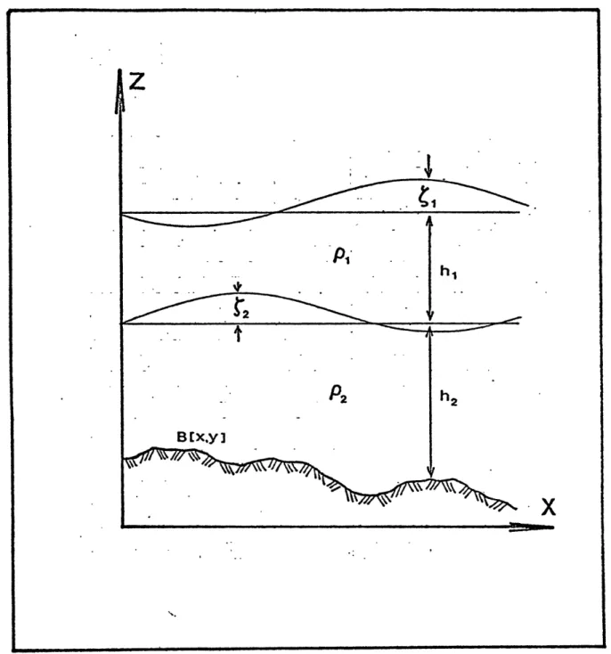
Frequently the ocean can be approximated by a two layer model. This occurs either when the upper layer of the ocean has been well-mixed
as a result of a storm or by the action of the trade winds or when it is heated during the summer months. In each case the thermocline is fairly abrupt and separates water masses above and below, each of which is almost homogeneous (see Fig. 2.1).
Let there be two layers of inviscid, incompressible homogeneous fluid, the lower one with density J2 and the upper one with density
, the bottom being described by the function b(x,y). The h's are the equilibrium thickness of each layer and the ' 's are the devia-tion of the surfaces from its equilibrium posidevia-tion. The equadevia-tion for the upper layer will be
(2.1.1)
-.-
.
.
1
...
(2.1.2)
dx
d(
(2.1.3)
-- d - _ _
=
~ 1 (2.1.4)- ' 22 1 5
...
--
---
(
2
.1
.6
)
This kind of problem was first investigated by Stokes (1847), (see for instance, Lamb, 1932, article 231). He solved for a wave propagating along the x axis with the upper surface of the upper fluid
free. For the special case where the depth of the lower fluid is great compared with the wavelength and the upper layer depth is much less than the wavelength he found
Cc
(2.1.7)The same solution was worked out in a very elegant fashion by Phillips (1966), solving the internal wave equation (1.2.3.10) with f=0 and
using a delta function for the Brunt-Vaisal'a function.
In view of the application of (2.1.7) to internal waves with semi-diurnal period over the continental shelf let us see the implication of the assumptions on this practical application. The continental shelf in
the region between Nova Scotia and Cape Hateras has a mean depth of 100 m. Very few internal waves were detected over the continental slope where
from 400 to 2200 m. This means, assuming h2 = 7xl 3cm, 1.01 > kh2 > 0.2 or that 5.07 coth kh2 > 1.25! So the assumption that coth kh2 = 1 is only approximately true for waves with smaller wavelengths, and if applied to larger wavelengths will give errors.
The other assumption was that the upper layer is much less than
3
-2-the wavelength or kh« (( 1, for hl = 3x10 cm. We have 8.57x10 Z kh1< 4.71x10~ , that can be considered a fair approximation. Now remains the question, can we neglect the Coriolis parameter f in the equations? What would be the consequences if we take it into account?
If we write down equation (1.2.3.10) again
g - N
=(2.1.8)
and the patching conditions,
r(-a*
a
)
=-(2.1.9)
and
where d + e is the depth of the discontinuity in density, so N(z) is zero outside this region. The solution of equation (2.1.8) and the conditions (2.1.9) and (2.1.10) lead to the dispersion relation:
2 *2
OC Pc'hO(~
)1R
where iM2 = q2 a2 2 2 and H is the depth of the flat bottom.
In this section, and when needed, we are going to choose our coordinates system such that our horizontal wave number a
=k
, can be thought of as in the x direction.Since one of our aims is to compute the depth of the mixed layer we need to work out the expression (2.1.11). The other aim is to compute
the amount of heat stored in the upper layer and as we shall see later on, only the velocity of propagation c is enough.
Under the assumption
Cofh
}-0
()
, consequentlyCo
h /4d
+ coft h
4( H-4 )
ca
+
-We can rewrite (2.1.11) as
and the expression for the mixed layer depth will be
C -1 C 0 L .
(c-
F 2- '2 fCI_______It is clear that if we make f=O and
ad
((
1 the expression (2.1.12) will reduce to (2.1.7). In Chapter 6 the results of computation of d using (2.1.12) and (2.1.7) will be discussed, but we aan anticipate that the inclusion of f does not change the results at all, of course for practical purposes.2.2 The Three-Layer Models
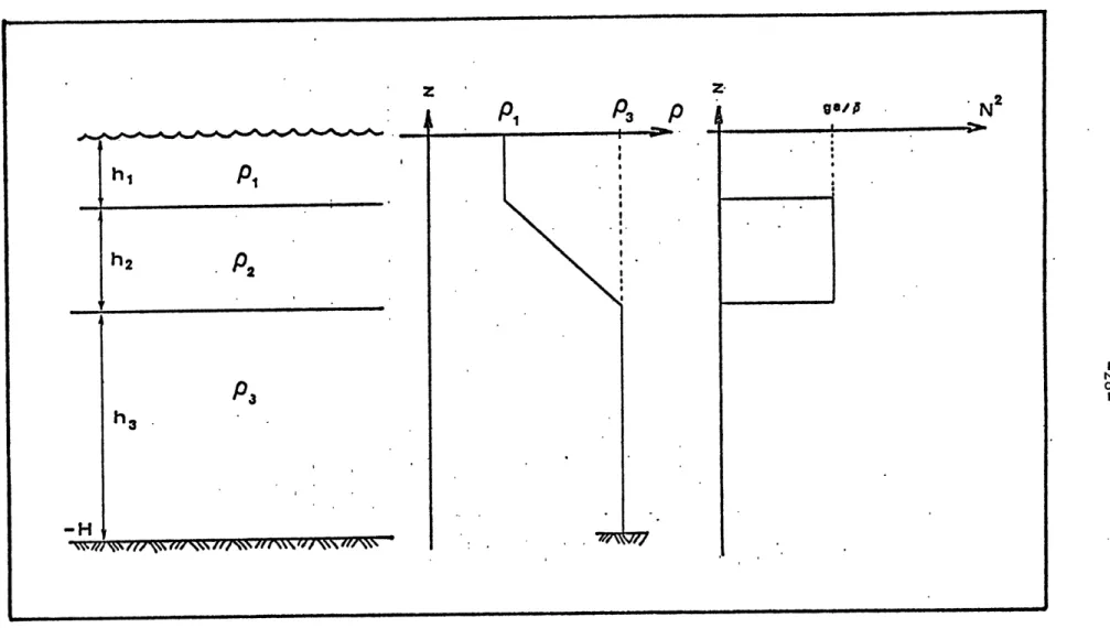
A more realistic model is a three-layer model with a density
pro-file and a Brunt-Vaisala frequency as shown in Figure 2.2. In the m6del the upper layer has a constant density pl, the bottom layer has a con-stant density p3, and in the middle we have a linearly varying density
profile like
(4, > 2
>
h+ h,
)
+ a (2.2.1) where 47/-/
/7,?The Brunt-Vaisala frequency in this layer is
= - .
2 3 + 0 h2
(2.2.2)
where g' = gAp/p is the reduced gravity for a two layer p1 and p3, and
where we have used a mean value (p 1 +P3)/2. Recalling the equation for vertical motions of internal waves (1.2.3.10)
h
2 .2
h
3.
-H
Figure 2.2 - The three-layer model, density distribution and
with the boundary conditions
Th solut=i '
=
o,-
'The solutions of (2.2.3) and (2.2.4) are:
W,
B,
si'A
2I
I
h3=
A
2 S z 13 t sinlJ-
A,
5 z <.
010
-h
2-
1<
f
< -6j
- H~ < h 2.
where the indices 1, 2 and 3 hold for the upper, middle and bottom layers and
I?
(14 2 z ?...
(rz Fa
To solve the problem completely we need four more conditions, that is, the conditions in the interface between the layers. The first one is that w must be continuous across the interface, i.e.,
[W]1-Z
'gt
2r., 41(2.2.9)
The second one is obtained by integration of (2.2.3) across the (2.2.4) (2.2.5) (2.2.6) (2.2.7) (2.2.8) -h,-A2 "
d
1
:0
(2.2.10)The application of these conditions to the solutions (2.2.5-7) gives rise to a set of homogeneous equations that admit a solution different from the trivial one, only if
Cos
S
0/A coshA
ki
CCos
0 (h
-sin Asin
S(h'
4.
- cos C; hcoS
J(h+ba
)
where h3 = H-h 1-h2. The above determinant
of the wave, -namely
is the dispersion relation
(
efoh2
(,ot/5h2 Y4 u 3i _. . f dnh - (2.2.11)where from (2.2.8)
N-a
(2.2. 12)
If we neglect the Coriolis parameter f the dispersion relation (2.2.11) can be rewritten as 0 0
-
coshj
b3
0
.ri7
(h,+
h
)
aDt ZZ=- h, ,-2-Y 21
4nhOk
)
0 (2.2.13)where now
S
=NZ
z ) ,=
and a is the wave number here considered only in the x direction for the sake of simplicity.According to Roberts (1975), care must be taken in making the Boussinesq approximation when this model of density distribution is used, particularly when a finite depth is assumed (Benjamin, 1967). It seems that the Boussinesq approximation is not valid for waves which are sufficiently long compared to the thermocline thickness h2
(Thorpe, 1968).~ Here we have solved separately for each layer so it is still valid to approximate
tanha hi a h1 tanh a h3 a h3
since a h1, a h3<< 1. But we cannot approximate the Cotan SA2 iln
(2.2.11), so
~2
2"
A
34
Yoe ('h.+b, )cofton
S=
2
(2.2.14)
factor the above dispersion relation and expanding small terms
1
((,+h
3)
?
(
.
C
=
(
N-
T)
b
3 (2.2.16)We see that even a first approximation of the dispersion relation for the three-layer model is useless for our purposes because it intro-duces variables that we cannot measure.
The first approximation for the group velocity will be
Ce = C ( i - *(2he 'A )
(2.2.15
3. DATA AND MEASUREMENTS
3.1 What the Internal Gravity Waves on the Continental Shelf Look Like
Surface manifestations of oceanic internal waves have been observed by many investigators, and their dependence upon wave-associated surface
currents has been recognized for at least a generation (Ewing, 1950). The surface signatures are most evident on a relatively calm sea and take the form of a quasi-periodic, long-length modulation of the capil-lary-ultragravity wave spectrum; the scale of the modulation is usually of the order of hundreds of meters (Gargett and Hughes, 1972). Visible manifestations on the ocean surface are theorized as being due to at least two mechanisms, either of which modulates the short surface wave structure rather than a change in optical reflectivity or absorptivity at depth. The first theory suggests that the high velocity of surface waves arising from the large internal wave amplitude sweeps together surface oils and debris to form a slick in regions of surface water convergence, thus increasing the specular reflection and decreasing the diffuse scattering over the convergence region.
On the other hand, Gargett and Hughes (1972) have suggested another mechanism based on the observation that surface waves seem to change
their direction of propagation over the crests of internal waves. They therefore investigated the interaction between surface waves and a periodic mean current induced by an internal wave. They found that if cgs(cos D )
>
c, over an internal wave crest, (cgs - surface wave group speed, c - internal wave phase speed, (D - angle betweenover an internal wave crest, i.e., if the surface wave groups are over-taken by the internal wave, the direction of the surface waves is turned away and their amplitudes decrease. Over troughs, the opposite effects occur. So for a given internal wave field, the system will have singu-larities for certain surface waves. Therefore, there will be regions where none of these surface waves can exist, and these regions will appear as surface slicks.
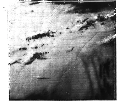
Periodic features observed in the United States eastern coast in certain ERTS A/B images have been identified as surface slicks, so associated with internal waves. These features are only present during northern hemisphere summer months, This suggests that these internal waves are present when summer solar heating stratifies the water suf-ficiently well to support such oscillations. When fall and winter wind action mixes the shelf water down to the bottom, the waves no longer appear. Figure 3.la and 3.1b show enlargements of ERTS images where internal wave manifestations can be seen.
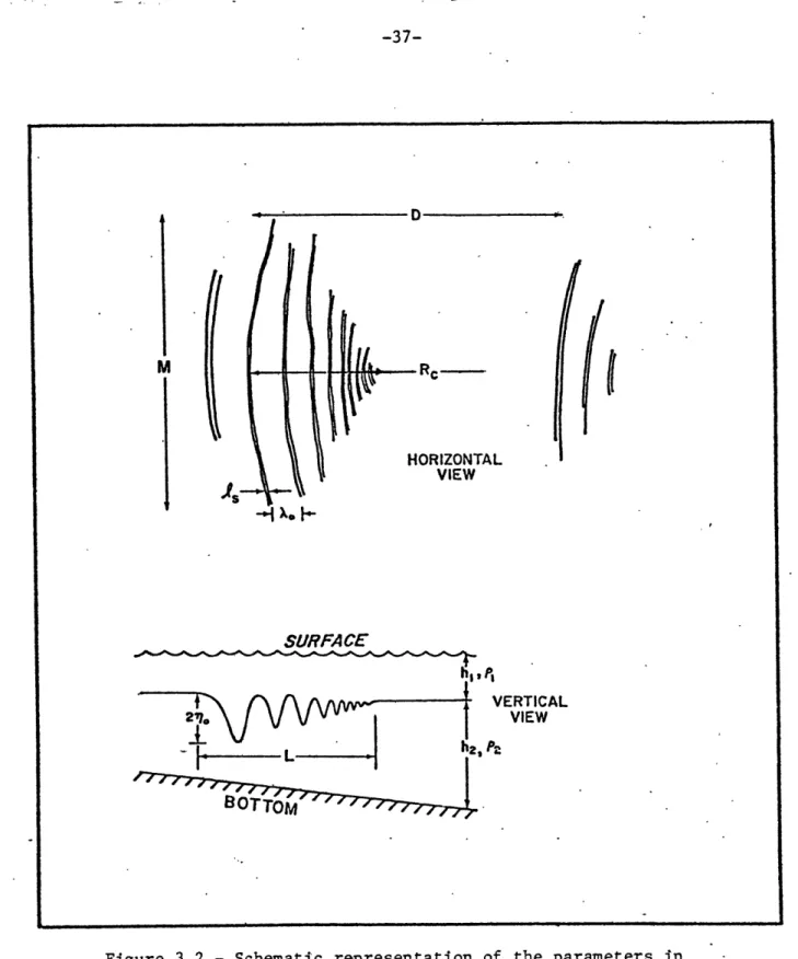
The common properties of these waves as they appear in these figures can be summarized as follows (Apel et al., 1974, 1975, 1976).
a) the waves occur in groups or packets of width L = 3 to 5 km, usually landward of the continental slope and separated by distances D, which range from 4 to 40 km;
b) the crests are nearly always oriented parallel to the local
bottom topography or can be loosely associated with some topographic feature seaward of their observed position, or both;
Figure 3.la - Enlargement of Landsat image 1364-14550 taken on 23 july 1973.We can see two wave packets north of Cape Ann; the waves propagate shoreward.
Figure 3.lb - Enlargement of Landsat image 1365-15013 taken on 23 july 1973.We can see two wave packets propagating towards the upper
decrease in wavelength, varying from ), at the front to X
<
)% at the back of the group;d) the lengths of the crests, M, fall between 5 to 100 km, with
a decrease in crest length occurring from front to back of the group; e) the widths of the slicks, ls, are often small compared to the lead wavelength Xo;
f) the crests are curved in a horizontal plane with their convex
sides pointed in the direction of propagation; the radii of curvature Rc, range from essentially infinity to a few kilometers;
g) as the packet progresses up on the shelf, there is some evidence
of a continued increase in the wavelengths throughout; this may be
accounted for by a combination of linear dispersion and nonlinear effects akin to solitary wave behavior.
All the parameters of the internal wave packets are shown in a
schematic way in Fig. 3.2.
Although there is no doubt about the identification of the above discussed features as internal waves, some non-users of satellite data can argue about the identification of the same. Here are some justi-fications (Apel and Charnel, 1976):
i) They exhibit the correct properties and behavior of internal waves.
ii) If they were surface waves, the average wavelength of 1000 m would imply a swell with the extremely long period of 24 sec and a
Figure 3.2 - Schematic representation of the parameters in an internal wave packet (After Apel et al. 1976).
the wind force must be 12 in Beaufort scale, Defant, Vol II, pg. 62), thereby eliminating surface waves possibility;
iii) Atmospheric internal waves as defined by clouds are certainly visible on ERTS-A/B Images. For these, the widths of the striations due to individual clouds are of the order 1/2 of wavelength while the
the pressured ocean striations have widths generally a small fraction of X . Furthermore, the latter are most visible when the atmosphere
is most cloud-free.
iv) Film or instrument artifacts have been eliminated by NASA/GSFC personnel (Apel and Charnel, 1974).
There is also the positive side of the question, that is also listed in the above referenced paper.
As to the sources and sinks for these internal waves, there is no doubt that they are "daughter" waves generated for a few hours during the peak current velocity by the long-wavelength baroclinic tide
occurring at the edges of the continental shelves. They then propagate with very low phase speeds, of order 0.2 to 0.5 m/sec to be absorbed
3.2 The Images, Climatological and Ground Truth Data
The primary source of data for the present work was the atlas of Sawyer and Apel (1976), which contains mozaics of images of LANDSAT satellite showing internal waves in the eastern coast of the United States. The images are second generation prints of ERTS images on photographic film. The scenes showing surface slicks to best advantage are usually those of channel 6 (600-700 nm) and occasionally channel 7
(700-800 nm). These scenes were enlarged to a scale 1:1,000,000 on high-contrast emulsion that enhanced the visibility of the slicks
(Apel and Sawyer, 1976). The wave packets are also plotted on a nauti-cal chart in the same snauti-cale as the satellite images.
A total of 78 measurements of the distance between two successive
wave trains were performed. The images exhibiting this phenomenum were taken during summer months, June, July and August of 1972, 1973 and 1974.
Figs. 3.la and 3.1b show enlargements of ERTS images where internal wave packets can be seen. These packets usually appear on the
continen-tal shelf, often in long lines parallel to the slope, leaving no doubt about their generation.
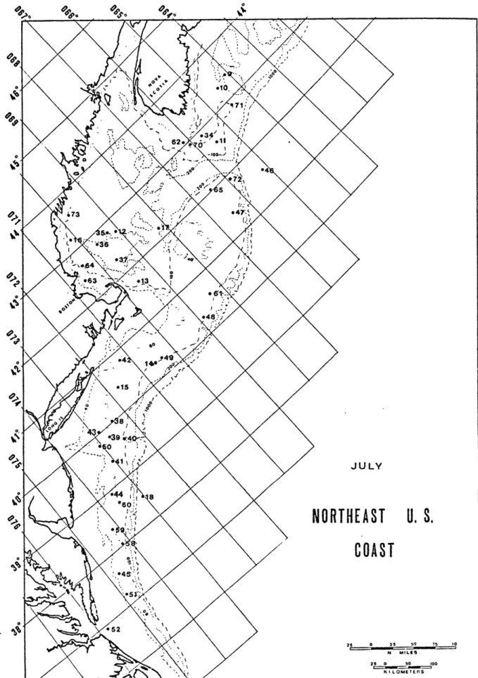
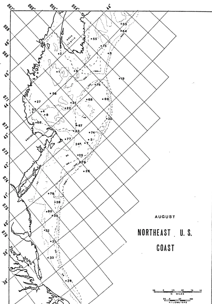
Since the interest is aimed at possible short-term variations, the data were divided according to the month of the event. The month of June had only very few measurements in the last days of the month, so there we added to the July set of data. For each event a point was selected such that it was located between the wave trains and at the middle of the distance D, defined in the previous section. These points are shown in Figs. 3.3 and 3.4 All data are summarized in Table I.
Figure 3.3 - Geographical distribution of internal waves observations for the month of July (1972, 1973 and 1974).
Figure 3.4 - Geographical distribution of internal waves observations
S at ".W a % --O we&A I. -4 4A WN-C "'' 40 W6400O6 644. 44' 4 Ota %4 0. 4W Om %a w0 0 ' 40 0N -4 -1400 0 -J "4- m 4.4 4 am0as -414 '-4 14 4 -1 4 -4 '1J 4-8 14 **I 4 4 -4 0-0 0 O00 0600 0M 0M00 0M00 -4 -4 4 -4 -4 4 -4 p40 olM00 00 o aa OaOmO NO N- 'O am paI.- 000001- # ' OOO aOtI-4t04wa4-N k4 a' 04-OO Wa414j N A,-. W I .I-4 TO 000 cc o-jo.4 00w 06 4 4004V009 1 R 664.4. N -0004 0 %00 4 4 .4~4 *.NIJO . 4 4 .4 ...--44 -4 .4 w N O 4.0o- 0 4644- '4 '4 '4 & %
~4-
.... . W4W8-W. . . . .WcaW . . . . . 44 W.. .e . -&-a- -. . ... W . .i . .64 W 4WW .. . . . . . . . 0 .4 .. p... . . . .4.. . . ... 64 l 100N 641 8 4-0 40 P04 . 4 0 -. 000 W.4 W Av 40. 0 At S-4 00 W 0, W 9p' W 0P 440 04 0' 4 W W . W 4W4W 0 W 4 0 N 4.4 -0' W.6 PN S. V' 04 S' !4 "1 F 00!, !4!4O D ON !* ON 4.4.4!.4 09 !,o.orO N0po p r 0 I? 44ae V N !4. N 404 NON N N r ?N r0 !4 v r p! N ON 6 40 :c4 Wa a g0 4A ba GO cr O w %a gy 00 Wke 01 O> 1a S-JP N a, w@ t a%>t mN w w wow -04wwo mwaGBP @@ta 4F.-" sor "cw w" .N -.O . .O6.0 .0 .O . O . . . 0.eL. . W w 1 . .P .In 4 . W W . . .0.e , Ne.0 . . .. NO N. O N ON. .. NN L4u aows 4 ^a % up w a t tA i. a, p- a 4 %ostamee -sm o w a 6 4 6%a4O 6 s t IF- 6, t Zeo 6%:41 o : a Z,.;- '4 '&A 'N1ON4 o ? W W, WN NW MN 4 N N N' N' N o.6 6% W W W W64 tN t4 0 a r acea m Q C0 0 6cNPNaPa a?, Ca% M N a Cor 47,0 wN . . .C % CN A r a or0% m 0P040 040 o N...e... QQQQQ Q . 4 0 % -04 &30 4 4 0.0 OW wwWW 0440064o4V-C &ow 4V- 4a4.NN0oN0N646" 400 646460 4. 4 4 . -0. 0 1 t4A 0% 40N a Lt0..M4. 4.NNNI'4 t N NNN 64 N NN N N N NN t*NN or -N 'I N 4 64 6e4 N 6- NN N 4.N 40 w NO-4um6w644404e me 4.600446 N-N 404400.N000'4N40OO4NO8-004 NN4'ONN4.04 mma0 P464000. 0 .10 !A !A 64 64A . .. .4 .4 .% .4 ib M L" W %A 'aU r a 4o 0 Da 4aa V .0 t O er L et ot 4s &O r ata -4 W 0 w -4 Da Q 01 01 -P- O 1a 00 W W 0-a Ma W O W Wo -4 W H ON P.- 01%,S Om t-Aa a, .. WThe other set of data used was climatological oceanographic data, which comprises mean monthly values of salinity and temperature at standard depths computed for each square of l* latitude by 10 longitude over the continental shelf from Cape Hatteras to Nova Scotia. Those squares with large number of data were subdivided into four
sub-squares
of 0.5* latitude by 0.5* longitude. Most of the data was kindly offered by V. Worthington of the Woods Hole Oceanographic Institution.Missing values at standard depths were replaced by those obtained by graphical interpolation. In few squares we have no values and these
were obtained from recent cruises in the months of July and August, through the National Oceanographic Data Center. Among these data is found what can be called ground truth data, i.e. hydrographic data taken at almost the same time as the satellite pass. Two of these are five days apart and the other two are fifteen days apart from the satellite pass. These were the best we could get.
3.3 Preliminary Analysis of the Measurements
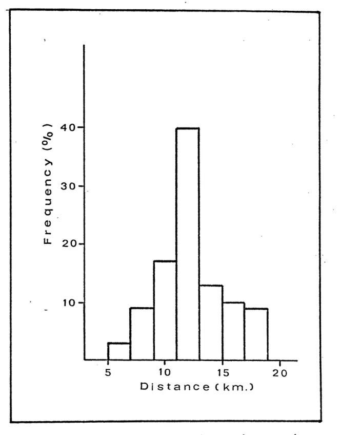
The measurements of the distance between successive wave packets taken from the satellite images is plotted in Fig. 3.5 as a histogram with 2 km interval. The distribution obtained suggests at least three dominant spacing multiples of a minimum spacing around 12 km.
The computations of the depth of the mixed layer (h) and of the heat stored (Q) based in the above measurements gave unrealistic results
for large spacings, just because h and
Q
vary as C We could ask -what is going wrong? But remembering that internal wave groups are only visible in surface images in the presence of capillary waves or shortFigure 3.5 - Histogram of the original distances between the successive wave packets (78 observations).
gravity waves, which only occur when there is wind, (Gargett and Hughes, 1972), the distribution can be interpreted to mean that there is only
one wave packet spacing in a given location during the period of the observations. This procedure assumes that the observation of multiple
of the minimal group spacing simply means that one has missed some groups since they are not visible because of an absence of surface ripples which can be modified by the internal wave velocity field. On this hypothesis, we assumed that there is a single wave packet spacing, and obtained
the histogram shown in Fig. 3.6 including all the wave packets measured. This interpretation may give an overly provable results, since it supresses variations from the mean longer than the mean, and since such values are modified by the stubraction of a multiple of the mean.
Over the continental shelf typical values for reduced gravity is g ~ (1)g cm-l For mixed layer depth it is h ~0(103)cm. This yields a typical velocity of propagation c ~ 0(30)cm sec~1 and a typical spacing
D - 0(14)km.
Another support for the Gausian type of distribution is wave trains found in overlapped satellite images. The ERTS overlapped images are taken 24 hours apart in time. A wave train identified in overlapping images are supposed to be 24 hours apart if there are no topographic features able to generate internal waves in the region. Waves satisfying these requirements were found and the distances between the packets
were at least 24 km, corroborating the hypothesis. The values of the depth of the mixed layer and the amount of heat stored were recalculated after. this procedure and the new values were quite reasonable.
40-0
C 30
-0 I-LL 2 0-
10-~. ~ S - 6 1Distance
(
km.)
Figure 3.6 - Histogram of the distance between the wave packets corrected by the multiples of the fundamemtal minimum distance (78 observations).
n
4. THE MIXED LAYER DEPTH IN THE OCEANS
4.1 The Stablishing Factors of the Depth of Mixed Layer
In the open ocean there is generally an isothermal surface layer which extends downward from the sea surface. The thickness of this
layer is the mixed-layer depth. In a region away from oceanographic boundaries and in the absence of turbulent mixing by strong currents, this depth is assumed to be influenced by two surface-induced processes -wind mixing (forced convection) and convective mixing (free convection). Wind mixing includes all the vertical turbulent mixing processes
resulting initially from the transfer of momentum from the wind to the sea. These are the mechanical mixings due to wave action (Laevastu, 1960), turbulent mixing due to the shear of drift currents (Ekman,
1905; Rossby and Montgomery, 1935; Munk and Anderson, 1948), and helical
vortices (Langmuir, 1938). Convective mixing occurs as a result of instability created at the surface by surface cooling and by evaporation of fresh water from the sea.
Another surface induced process, if we neglect the effect of diffu-sion, is the entrainment responsible for the exchange with the water below. The entrainment flow can only be directed towards the more tur-bulent fluid region, that is, upwards in the present case, cooling and
increasing the density of the upper layer. In the absence of entrainment, all the turbulent fluxes become zero at the boundary. This means phy-sically that there is just not enough turbulence energy available to overcome the stable stratification at the base of the layer to produce any mixing with the lower water.
Although it is generally accepted that both forced and free con-vection are important factors influencing the upper mixed layer, wind mixing can be considered to be the main factor in the considered region
and time of the year; convective mixing is assumed to be the secondary. Tabata et.al. (1965) showed that there is a linear relation between the mean wind speed averaged 12 hours in advance of the bathythermo-graph observation and the depth of the summer isothermal surface layer at ocean station P.
In the region considered here the currents over the continental shelf are mainly driven by the meteorological conditions and the drift velocities range from 5 to 25 cm sec (Bumpus and Lauzier, 1965), and can be considered weak. We can say that the transport of surface
waters have little effect on the properties of the water, but horizontal and vertical mixing are dominant (Ketchum and Corwin, 1964). Thus we
can assume the interaction between the sea and the atmosphere to be the dominant factor affecting the upper layers of the ocean in the studied region.
4.2 Estimation of the Mixed Layer Depth 4.2.1 From 2-Layer Model
An application of the results derived in sections 2.1 and 2.2 will be discussed here. The velocity of propagation of the interfacial wave
is
2llo
c',
- j-t.1
h,
(4.2.1.1)
From this relation it is seen that if we know the velocity of propagation c, the density difference Ap, and the density of the lower layer p2' it will be possible to compute the depth of the interface hl that we will call mixed layer depth.
The velocity c can be estimated from the distance between two consecutive trains of waves in the satellite images, and assuming they are 12.4 h apart in time (semi-diurnal period), the difference in density Ap and p2 can be obtained from climatological data. The acceleration
of gravity can be assumed to be 980.665 cm sec -2. Table I shows the result of the computation of hl using the relation
(see also Table I,)
hc
(3.2.1.3)
The values computed using the above equation differ only slightly from those computed from (4.2.1.2), and for practical purposes they can be considered equal. So it is perfectly right to neglect f in the dynamical equations.
Computed values of the depth of the mixed layer were plotted over a chart of the New England continental shelf for the month of July
and August and are shown in Figs 4.1 and 4.2.
4.2.2 Comparison with Ground Truth Data.
A comparison between the depth of the mixed layer computed using
the expression (4.2.1.1) and the ground truth observations was made. The closest hydrographic observations performed to the satellite pass are shown in Figure 4.3. From this figure we can estimate the depth of the mixed layer. We took as mixed layer depth the depth just before the pycnocline. Table II shows the results of the comparison.
We must have in mind that the standard depth for sampling in hydro'graphy are 0 m, 10 m, 25 m, ... when using Nansem bottles.
Figure 4.1 - Mixed layer depth computed from satellite observations of internal waves for the month of July (1972, 1973
Figure 4.2 - Mixed layer depth computed from satellite observations of internal waves for the month of August (1972, 1973 and 1974).
Figure 4.3 - Density profiles taken from hydrographic observations used as ground truth.
HYDRO COST IN SPACE AND TIME.
Date Latitude Longitude
h (m)
Q
(k cal cm)-2 sat obs #65 07-19-73 42.01*N 066.30*W 23 6.23 hydro obs B-4 07-14-73 42026 N 066013 W 30 9.98 sat obs #70 06-27-74 42.57*N 066.03*W 36 3.51 hydro obs C-7 07-11-74 43003 N 066053 W 26 5.04 sat obs #62 07-19-73 43.02*N 066.06*W 10 1.56 hydro obs B-5 07-14-73 42042 N 066.40 W 9 3.56 sat obs #76 08-02-74 42.50*N 066.40*W 24 6.24 hydro obs C-4 07-13-74 42031 N 066011 W 20 9.30Consequently if we have a sharp pycnocline between 0 and 10 meters we can not recognize it by plotting the standard depth values. This means that a lower value of mixed depth layer, computed by (4.2.1.1),
An extremely important component of the earth's heat balance is the storage of heat in the summer hemisphere and its release in the winter hemisphere. Except in certain land areas where a considerable
seasonal fluctuation in soil moisture takes place, heat storage is severely limited by the comparatively slow rate of heat conduction in the solid earth. The relatively low heat capacity of air restricts seasonal heat storage by the atmosphere. The hydrosphere, on the other hand, is partly transparent to short-wave radiation, has a great heat capacity, and is in nearly constant turbulent motion. It is
able, therefore, to play a dominant role in seasonal heat storage. The heat stored in the seasonal upper warm layer of the oceans comes from solar radiative input and is in part balanced by losses to the atmosphere in the form of radiation and diffusion of sensible heat and latent heat of evaporation, as well as turbulent exchanges with deeper layers of the ocean. These processes, balanced by
hori-zontal advection, determine the temperature, depth and the salinity of the upper layer, the time of layer formation in the spring, and the overturning and disappearance of the layer in late fall.
The heat stored in the upper ocean affects, both climatologically and synoptically, the weather development and the mixing processes in the layer driven by wind and thermal effects also transport oxygen, nutrients and biota. Observations indicate that seasonal heat storage
takes place in the upper one hundred to one hundred and fifty meters of the ocean.
5.2 Heat Stored Calculations from In-Situ Measurements
The heat flux from the atmosphere through the sea surface ends up in different ways:
a) it may raise the temperature of the ocean column, b) it may be carried away by horizontal advection, or
c) it may be exchanged with deep colder layer.
The above processes actually occur simultaneously in the ocean.
The annual heating cycle of the water column over the continental shelf is well known, and as examples we have Figures 5.la, 5.lb and 5.lc. These figures show the variation of the mean monthly values of temperature of the upper water column from the early spring to late summer for three representative regions of the eastern continental
shelf. These regions cover three squares where we have some internal wave observations. Figure 5.la shows the temperature profiles for the
square (42-43)*N x (065-066)*W, covering the entrance and the north part of the Northeast Channel, Gulf of Maine. Figure 5.1b shows the profiles for the equare (40-41)*N x (068-069)*W, covering the region of the continental shelf and continental slope east of Cape Cod. Figure 5.lc shows profiles of the equare (37-38)*N x (074-075)*W
covering the continental shelf and slope off Delaware and Maryland. From these figures we notice that the water is heated from a minimum temperature profile To(z) (March), to a maximum profile that
could be August or September. As already pointed out in Chapter 5 we can neglect the advected heat, and here we are also going to neglect
Figure 5.la - The annual heating cycle of the upper ocean from the region (42-43)*N and (065-066)*W.
TEMPERATURE (*C) 4 6 8 10 12 14 16 w
0
O -150 200 250 18 20Figure 5.1b - The annual heating cycle of the upper ocean for the regions (40-41)*N and (068-069)*W.
MAR A 50 01 100-C I 2.5150 100-' 8 io 1 18) 20d 22 2 APRA
i7
i/ a. - U-I
I!
250-Figure 5.1.c -The annual heating cycle of the upper ocean for the region (37-38)* and (074-075)*W.
heat contained in the upper layer of the ocean as the heat accumulated from the minimum temperature profile To(z) to a given profile T(z) in absence of advection and exchange with water below as
f oz) p ,.(z , [ ci;(5.2.1) -h
where p is the density of the sea water, c is the specific heat at constant pressure and h is the depth of the thermocline. When using this definition we must be aware that we are overestimating its value. To overcome this overestimation instead of using To(z) for the month of March, we have chosen the minimum profile two months latter.
5.3 Heat Storage Calculations from Satellite Images
5.3.1 Based on Two-Layer Model
The most important application of the internal wave images from satellites is without doubt the fact that we can actually compute the amount of heat stored in the upper layer using only the velocity of propagation of the packets. Let us see how this can be done. Start with the amount of heat stored defined as
since we are dealing with a two-layer ocean,
/Sf-
(S .o<T-(5.3.2)
The above assumption is critical because in estuaries, for example, the density is controlled mainly by the salinity gradient.
Figure 5.2 is a plot of values of -aAT against SAS, for the regions shown in the chart inside the figure. Besides the point drawn as an open circle, the other points indeed support the assumption that SAS is not so important as -oaT in account for density changes.
The anomalous point describes the density changes for the coastal region east of Delaware, being under the influence of the Chesapeake Bay waters. Since we did not plot points for all regions we can expect
the same behavior for coastal regions in the vicinity of large river mouths. Fortunately there are very few internal wave observations under such conditions. After all, these regions are no problem because we can overcome this fact by taking into account the salinity dependence
by determining a function g=g(T,S) through a T,S relationship for these
regions and still keep a linear dependence on temperature. This proce-dure would also improve the determination of the density in other
regions. From (2.1.7)
.C.
-oA
'D
G
B
L.
K.
-3.0
-2.11
J
.-
1.a
__________________IPAS
-2.0
-1.0
1.0
Figure 5.2 - Values values in theof -aAT and SAS from mean monthly of T and S for the regions shown
AP
&( T
(5.3.4) 2
Combining the relations (5.3.4), (5.3.3) and (5.3.1) and also assuming p1 ~. p2, which numerically will not make any computational difference, we get
P,
:PC (5.3.5)
The expression (5.3.5) gives us in cal cm -2, if we use cgs units, the amount of heat stored in the upper layer, under the above assumptions.
2
Assuming c , g and a constants, the only variables are c , that is measurable from satellite images, and p2 that can be inferred from
climatological data.
The motivation to use p2 instead of p1 is that, although both are
of order 1, the former one is less subject to small term variations than the last one.
The comparison with the scarce ground truth data available is shown in Figure 5.3. The values of heat stored inferred from satellite observations are less than the one computed from in-situ data and this will be discussed later. Charts of the heat stored in the upper layer over the New England continental shelf for the month of July and August are shown in Figures 5.4 and 5.5.
10
8
E
6-o--0
.
2
4
6
8
Qsat.( kcal /cm
2)
Figure 5.3 - Comparison of stored heat computed from satellite observations (Q .sat.) of internal waves and those computed from in-situ data (Q ).ins
Figure 5.5 - Amount of heat stored computed from satellite observations of internal waves for the month


![[PDF] Cours Microsoft Word 2007 comment ça marche | Cours informatique](data:image/gif;base64,R0lGODlhAQABAIAAAP///wAAACH5BAEAAAAALAAAAAABAAEAAAICRAEAOw==)