HAL Id: hal-02946371
https://hal.archives-ouvertes.fr/hal-02946371
Submitted on 23 Sep 2020
HAL is a multi-disciplinary open access
archive for the deposit and dissemination of
sci-entific research documents, whether they are
pub-lished or not. The documents may come from
teaching and research institutions in France or
abroad, or from public or private research centers.
L’archive ouverte pluridisciplinaire HAL, est
destinée au dépôt et à la diffusion de documents
scientifiques de niveau recherche, publiés ou non,
émanant des établissements d’enseignement et de
recherche français ou étrangers, des laboratoires
publics ou privés.
Diffusion MRI fiber orientation distribution function
estimation using voxel-wise spherical U-net
Sara Sedlar, Théodore Papadopoulo, Rachid Deriche, Samuel
Deslauriers-Gauthier
To cite this version:
Sara Sedlar, Théodore Papadopoulo, Rachid Deriche, Samuel Deslauriers-Gauthier. Diffusion MRI
fiber orientation distribution function estimation using voxel-wise spherical U-net. International
MIC-CAI Workshop 2020 - Computational Diffusion MRI, Oct 2020, Lima, Peru. �hal-02946371�
function estimation using voxel-wise spherical
U-net
Sara Sedlar, Th´eodore Papadopoulo, Rachid Deriche, and Samuel Deslauriers-Gauthier
Inria Sophia Antipolis-M´editerran´ee, Universit´e Cˆote d’Azur, FR Athena Project-Team
Abstract. Diffusion Magnetic Resonance Imaging (dMRI) is an imag-ing technique which enables analysis of the brain tissue at a microscopic scale, particularly the analysis of white matter. Given a high enough an-gular resolution, a common way to explain the measured signal is via fiber orientation distribution function (fODF). This function describes the orientation and volume fraction of axon bundles within each voxel and is an essential ingredient of tractography. In this work, we have in-vestigated a deep learning approach for the fODF estimation. U-nets enable fast and high resolution inference by combining multi-scale fea-tures from contracting and expanding parts of the network. As dMRI signals are most commonly acquired on spheres, we propose a spherical U-net which is adjusted to the properties of the dMRI data, namely its real nature, antipodal symmetry, uniform sampling and axial symmetry of the signals corresponding to individual fibers. We compared our model with another deep learning approach based on a 3D convolutional neural network and a state-of-the-art approach - multi-shell multi-tissue con-strained spherical deconvolution, on real data from Human Connectome Project and synthetic data generated using ball and stick model. The methods are compared in terms of mean square error and mean angular error for dMRI signals of different angular resolutions. Provided quan-titative analyses show improved performance with our approach even with significantly reduced number of parameters and results obtained on synthetic data indicate its robustness with respect to noise. Qualitative results illustrating the performance of the methods are also presented. Keywords: diffusion MRI · fiber orientation distribution function · spher-ical U-net
1
Introduction
Diffusion MRI is an imaging modality tailored to capture interactions of diffus-ing water molecules with surrounddiffus-ing micro-structures within examined tissue. As such, it has shown importance in neuroimaging, particularly in the analysis of white matter micro-structures . It opened the possibility to examine proper-ties of axon bundles such as orientation, volume fraction, dispersion, etc. Models
proposed to explain the dMRI signals have evolved with the improvement of the acquisition process. Initially, in Diffusion Tensor Imaging [1], axon bundles were described via diffusion tensors [2]. With the increase of dMRI angular resolution, more informative models have been proposed, specifically in voxels containing crossing or kissing fibers, fiber fanning or bending. A number of these mod-els include estimation of probability density functions (PDF) such as Ensemble Average Propagator (EAP) [3,4] describing average relative spin displacements, diffusion Orientation Distribution Function (dODF) [5,6] and fiber Orientation Distribution Function (fODF) [7,8,9]. These voxel-wise quantities opened the possibility of tracking white matter pathways - tractography [10], a process of a great potential in the analysis of brain structural connectivity [11].
The fODF is a spherical PDF that reveals orientations and volumes of the un-derlying axon bundles. Traditional methods include estimation of a single fiber response function that is deconvolved from the dMRI signal in order to obtain the fODF [7,8,9].
Recently, a 3D convolutional neural network (3DCNN) directly applied on spher-ical harmonic (SH) coefficients has been proposed for the fast estimation of fODFs [12]. In [13], for the same problem, residual CNN (ResCNN) and dense neural network (ResDNN) have been investigated. In both works, potential of the models has been demonstrated for significantly downsampled acquisition sampling schemes, what is often a requirement in clinical applications.
U-nets have shown potential in high resolution inference from planar data by combining multi-scale features from contracting and expanding parts of the net-work [14]. As sampling of dMRI signals is most commonly performed on spheres, all building blocks of U-net need to be adjusted to the properties of spherical signals. Recently, in [15], a spherical U-net has been proposed for the cortical surface parcellation and prediction of attribute maps, with convolutions, pooling and transposed convolutions adjusted to the spherical space. A neural network model, similar to the planar CNN, for the analysis of spherical data - spherical CNN (S2CN N ) has been introduced in [16], where, contrary to [15], in order
to avoid computationally expensive interpolations, convolutions of signals and kernels are performed in spectral domain. Similar approach has been developed in [17], where a significant speed up of convolutions has been achieved with zonal kernels.
In this work, we have addressed the problem of the fODF estimation from dMRI data acquired with significantly downsampled acquisition schemes. Exploiting the properties of the U-net and S2CN N , we propose a voxel-wise spherical
U-net, that is tailored to the properties of dMRI signals acquired on spheres, namely real nature, uniform distribution of samples, antipodal and axial symmetry of the signals generated by individual fibers.
2
Background and method
The main operations in U-nets are convolutions, pooling, and transposed con-volutions. While the convolution of equidistantly discretized planar signals with
kernels is well defined, convolution between S2 signals and kernels faces two
challenges. First of all, the operation analogue to the translation in Euclidean space during convolution is not a rotation in S2 space, but in the SO(3)
man-ifold. Secondly, the discretization of signals in Euclidean space is usually done in an equidistant manner, what cannot be achieved in S2domain. An
interpola-tion must therefore be performed for each step of convoluinterpola-tion. These problems are addressed in the work presented in [16] where the spherical CNN - S2CN N
has been introduced. In this framework, to avoid the computationally expensive interpolations, convolutions of S2and SO(3) signals and kernels are performed in spectral domain, and as in standard CNNs, activation function is applied in signal domain. Furthermore, to achieve the same effect as pooling, in each new layer, the bandwidth of the input signal is reduced and the support of the kernel is spread. In [17], additional speed up has been achieved by constraining kernels to be zonal. As a consequence, the convolution can be more efficiently performed in S2. In this work, we propose a spherical U-net with convolutional building
blocks from [16,17] adjusted to the properties of dMRI data.
Given the antipodal symmetry of the dMRI signals, we use only the SH basis of even degree for their representation. A signal s : (θ, φ) → R can be written as
s(θ, φ) = Lmax X l=0 m=l X m=−l ˆ sml Ylm(θ, φ), for l ∈ {0, 2, ..., Lmax} (1)
where θ and φ are inclination and azimuth angles, Ym
l (θ, φ) are SH basis of
order m and degree l, and ˆsm
l are the corresponding SH coefficients. Lmax is the
signal’s bandwidth determined as
N ≥ (Lmax+ 1)(Lmax+ 2)/2 (2)
where N is the number of sampling points. In addition, as dMRI signals are real, we reduce computational complexity by using the real SH basis
Ylm= √ 2(−1)mIm[Yl|m|] if m < 0 Y0 l if m = 0 √ 2(−1)mRe[Ylm] if m > 0 . (3)
Consequently, spherical kernels are also real and antipodally symmetric. Another important property of dMRI signals is the axial symmetry of the signals coming from individual axon bundles. This motivated us to use kernels that are axially symmetric around z axis - zonal kernels and in this way promote an axon bundle-wise feature extraction. Zonal kernels have been introduced in [17] in order to decrease the computational complexity imposed by performing convolutions of SO(3) signals and kernels as in [16]. Given this, kernel h : (θ) → R can be represented as a linear combination of zonal harmonics (ZH) as
h(θ) = Lmax X l=0 ˆ hlYl0(θ, 0), for l ∈ {0, 2, ..., Lmax}. (4)
This significantly simplifies convolution between signals and kernels, as the re-sulting signal is no longer in SO(3) manifold, but in S2 space. In addition,
since the number of ZHs necessary to represent such kernels is rather small -Lmax/2 + 1, we used directly ZH coefficients as trainable parameters as it was
initially introduced in [17]. Convolution between a signal s : (θ, φ) → R and an axially symmetric kernel h : (θ) → R, represented with ZH coefficients ˆhlcan be
written as c(θ, φ) = Lmax X l=0 ˆ hl m=l X m=−l ˆ sml Ylm(θ, φ), for l ∈ {0, 2, ..., Lmax}. (5)
As we are dealing with discrete signals, Eq. 1 can be simply written as matrix-vector product as s = Y ˆs, where Y contains SH basis Ylm(θk, φk) in columns,
sampled at the angles (θk, φk), ˆs are corresponding SH coefficients and s is a
discrete spherical signal. Although the discretization of the band-limited planar signals without information loss is well defined with Nyquist-Shannon sampling theorem and their transformation to spectral domain is trivial, discretization of the spherical signals and calculation/estimation of SH coefficients is a challenging task. Sampling theorem for band-limited spherical signals has been introduced in the work of Driscoll and Healy [18], where they have defined an equiangular sampling grid that guarantees information preservation and calculation of SH coefficients. The total number of required samples is N = 4(Lmax+ 1)2. Given a
signal sampled on Driscoll-Heally grid, s : (θk, φk) → R and SH basis discretized
in the same way in a matrix Y , calculation of SH coefficients can be simply writ-ten as ˆs = W YHs, where H refers to conjugate transpose and W are quadrature weights necessary to account for the basis orthogonality loss due to discretiza-tion. This sampling is quite excessive and given a real world situation where a signal is not completely band-limited and is affected by noise, signal segments around poles that are oversampled would be more accurately represented. Due to this, sampling on a sphere is, in general, application dependent and dMRI signals are usually sampled uniformly over multiple shells in a way that an opti-mal angular coverage is achieved [28]. As a consequence, some information can be lost and several methods for the estimation of SH coefficients have been pro-posed [19,20,21]. In this work, we have used Gram-Schmidt orthonormalization process to estimate the basis Y0for the transformation of S2signals into spectral
domain, similarly as introduced by Yeo [19]. This is performed in an iterative manner, if yi and y0i correspond to i − th columns of Y and Y0, respectively, y0i
are determined as follows:
yi0 = yi− i−1 X j=0 hyi, y0ji hy0 j, yj0i yj0, y0i= y 0 i ||y0 i||2 . (6)
where y00= y0. In this iterative process, as we start from basis that correspond
to lower frequencies, more importance is given to them. This is convenient as we know that aliasing affects higher frequencies. In order to avoid bias due to ordering of the basis, Gram-Schmidt process is repeated multiple times, each
time randomly shuffling the order of the basis of the same degree, which are at the end averaged. SH coefficients are simply estimated as ˆs = Y0Ts.
Voxel-wise spherical U-net Figure 1 depicts an illustration of the proposed spherical U-net. Input to the U-net is composed of n3·n
shellsdiscrete S2channels,
where n is the size of neighbourhood and nshells is the number of dMRI shells.
Output corresponds to the SH coefficients of the estimated fODF. We refer to the results of (transposed) convolution of input S2 signals and zonal kernels,
followed by activation function, as feature maps, which are sampled at uniformly distributed points on sphere, generated using Q-sampling tool [28]. The network is composed of contracting and expanding parts. Each layer of the contracting part extracts feature maps that are of the same bandwidth as its input (that is used as a part of the input to the parallel layer in the expanding part, black horizontal arrows in Figure 1) and corresponding feature maps with decreased bandwidth that serve as the input to the following layer of the contracting part (pink arrows oriented down in Figure 1). The decrease in bandwidth imitates pooling of the planar CNNs. Feature maps of the same bandwidth are computed as convolution of signals/feature maps transformed into spectral domain and kernels, represented with ZH coefficients, as in Eq. 5, followed by Rectified Linear Unit (ReLU) activation function. These feature maps are further transformed into spectral domain with decreased bandwidth and serves as the input to the following layer of the contracting part. Each layer of the expanding part learns up-sampling of the feature maps which serve as the input to the following layer in the expanding chain or as the final inference. In general, as input, it receives the feature maps from the parallel layer of the contracting part, if such layer exists (black horizontal arrows in Figure 1) and the feature maps estimated by the previous layer of the expanding part (turquoise arrows oriented up in Figure 1). Transposed convolution in planar CNN simply corresponds to the insertion of zeros between points and convolution with kernels. We have implemented the transposed convolution as follows
– Let Ni be the number of sampling points of the input feature maps of layer
i with bandwidth Limaxdetermined according to inequality 2.
– To up-sample the feature maps from layer i to layer i − 1 to have bandwidth
L(i−1)max, we first generate Ni−1 sampling points using Q-space sampling tool
[28] and compute the corresponding basis Y0 as in Eq. 6.
– Since Q-space sampling points are generated incrementally, positions of the points of the layer i correspond to the first Nipoints of the sampling scheme
of the layer i − 1, so inserted zeros correspond to the last Ni−1− Ni points.
– Up-sampled SH coefficients are computed as ˆsi−1= Y:,1:N0T isi, where :, 1 : Ni refers to the cropping of the matrix Y0T to N
i columns.
– Convolution of the up-sampled signals and kernels is performed as in Eq. 5 followed by an activation function.
Conv (eq. 5 ) +ReLU
Upsampling + FT + conv (eq. 5) + ReLU + FT + FT concatenation fODF LmaxfODF Lmax1 nfm 1( c) +nfm 1 ( e) nfm 0 nfm 1( c) Lmax1 nfm2( c)+nfm2( e) Lmax 2 nch 1 Lmax3 nfm3( c)+nfm3 (e) nfm 4 ( e) Lmax 4 nfm 4 ( c) Lmax 4 Lmax 2 nfm2( c) Lmax3 nfm3( c) ⋰ dMRI signals 3 shells n×n×n 1 2 nch=n 3 ⋅nshells Fourier transform (FT)
Lowpass + Conv (eq. 5 ) +ReLU
nchnumber of input channels nfmi( c)/nfmi(e)number of feature maps in i
th layer of contracting and expanding parts Lmax
i
signal/feature map bandwidth in ith layer nshellsnumber of dMRI shells
input neighborhood size n×n×n
Fig. 1. Illustration of a spherical U-net architecture with corresponding convolutional operations in contracting and expanding parts
3
Dataset
We used in our experiments two types of datasets, real data from Human Con-nectome Project (HCP) [22] (referred to as Real dataset ) and synthetic data gen-erated from the same real HCP scans using multi-fiber ball and stick biophysical model [23] following the procedure described in [24]. Real data was acquired on Siemens 3T Skyra system with 100 mT /m gradient, over three shells with b-values of 1000, 2000 and 3000 s/mm2, each with 90 gradient directions and
18 b = 0 images at resolution 1.25x1.25x1.25 mm3. To generate synthetic data,
first, up to three fiber orientations and corresponding volume fractions were estimated per voxel using the bedpostx tool from the FSL library [25]. These parameters were then used to generate synthetic data using the multi-fiber ball and stick model as in [24] for each shell independently. In the generation process, the free diffusivity coefficients are set to {0.68, 0.96, 2.25} · 10−3s/mm2 for the white matter, gray matter and cerebrospinal fluid, respectively [24]. Single-fiber tensor’s eigenvalues are set to {λ1, λ2, λ3} = {1.7, 0.17, 0.17} · 10−3s/mm2 [24].
To simulate more realistic dMRI data, Rician noise with SNR=18 was added to the synthesized data. In addition, in order to investigate the robustness of the compared methods, one synthetic dataset is generated with the constant diffu-sion single-fiber tensor eigenvalues (Synthetic dataset 1 ) as in [24] and another one with the eigenvalues taken from the uniform distribution around these val-ues (valval-ues taken from the range of ±10%) (Synthetic dataset 2 ). Experiments are conducted on Real dataset, Synthetic dataset 1 and Synthetic dataset 2 with downsampled acquisition schemes. To select relevant white matter voxels, we used brain tissue segmentation computed from T1w images using the FAST
al-gorithm [26] implemented in the mrtrix library [27]. Gold standard fODFs, of SH degree 8, were estimated using the multi-shell multi-color constrained spherical deconvolution (MSMT-CSD) approach [9], on signals acquired on full sampling scheme, using mrtrix library [27]. In the case of synthetic data, fODFs were es-timated on the noise-less data. We used 50 subjects in total, 30 for training, 10 for validation and 10 for testing.
4
Experiments and implementation details
In order to evaluate our method on data similar to those used in clinical prac-tice, experiments are performed on data with significantly reduced number of sampling points Np (20, 30, 40, 60, 90 and 120 in total for the three shells). We
compared our method with another deep learning approach - 3DCNN [12] and with MSMT-CSD [9]. To investigate importance of neighbourhood information, our model is trained with single voxel multi-shell (S2U -net1×1×1) signals and
with 3 × 3 × 3 neighbourhood multi-shell input (S2U -net3×3×3), what is also
the case with the 3DCNN model. In addition, to investigate potential of our approach, we trained one model with significantly lower number of trainable pa-rameters - S2U -net3×3×3
s . Sizes of the deep learning networks are given in Table
1. Both deep learning approaches are implemented using the tensorflow library
Table 1. Sizes of 3DCN N s and S2U -nets (MB) for Np sampling points.
Model / Np 20 30 40 60 90 120
3DCN N 18.12 18.12 18.12 18.96 20.18 20.18 S2U -net1×1×115.65 15.65 15.65 19.30 20.52 20.52
S2U -net3×3×3s 3.99 3.99 3.99 4.89 5.17 5.17
S2U -net3×3×315.80 15.80 15.80 19.42 20.60 20.60
[29]. Models are trained over 100 epochs. In each epoch, 3 dMRI samples are randomly selected from 30 training samples. For both models loss function is de-fined as mean square error (MSE) between estimated and gold standard fODFs represented in spectral domain. Initial learning rate is 0.001 and after 50 epochs it is reduced to 0.0001. Model weights updates are computed using the Adam optimization algorithm [30].
5
Results and conclusions
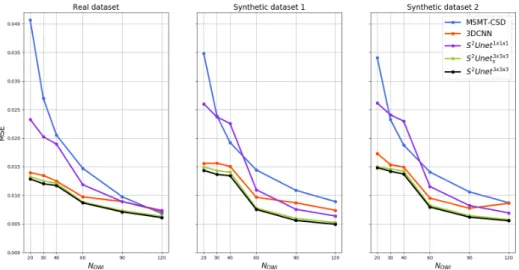
Results are compared quantitatively in terms of MSE and mean angular er-ror (MAE) for single fiber voxels and voxels containing two crossing fibers. To compute peaks of the estimated and gold standard fODFs we used the mrtrix library [27] and the threshold of 0.1 of the highest peak is used to eliminate spurious fibers. In Figure 2 we can see that our models S2U -net3×3×3 achieve
significantly lower MSE compared to the models that do not use neighbouring information and slightly, but consistently lower MSE compared to 3DCN N . In addition, almost equal performance can be achieved with a more compact model - S2U -net3×3×3
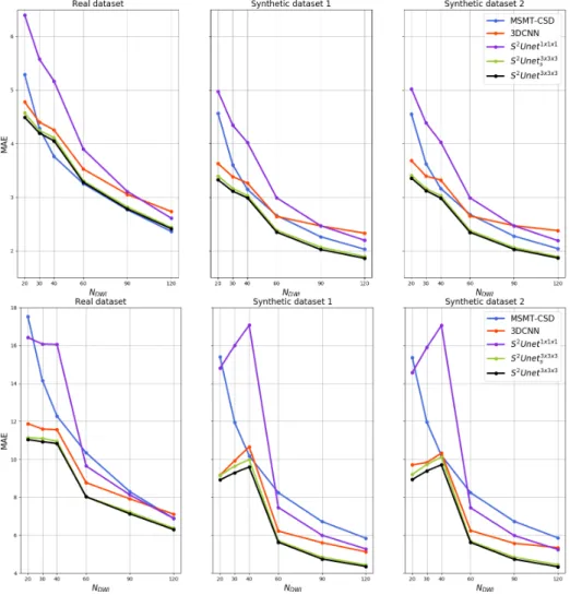
s . In Figure 3 we can notice that for single fiber voxels and real
dataset, MAE is almost equal to the one achieved with MSMT-CSD, however the results obtained on synthetic data indicate that our approach is more ro-bust to noise. As depicted in Figure 3, S2U -net3×3×3and S2U -net3×3×3
s achieve
lower MAE in voxels with crossing fibers. Qualitative comparison of MSMT-CSD, 3DCNN and S2U -net3×3×3is provided in Figure 4 for 60 sampling points. We can notice that MSMT-CSD compared to the 3DCNN and S2U -net3×3×3is more prone to produce spurious fibers, while these deep learning approaches are more likely to omit some.
Fig. 2. Comparison of MSE averaged over 10 testing subjects for real HCP dataset, Synthetic dataset 1 and Synthetic dataset 2 for different number of sampling points.
In this work we have proposed a deep learning method that is adjusted to the properties of dMRI signals, namely real and spherical nature of the signals, antipodal symmetry, random distribution of the sampling points and axial sym-metry of signals coming from individual fibers. We have demonstrated that the proposed method is suitable for high resolution inference such as the estimation of the fODFs and can successfully incorporate neighbouring information to boost its performance. Compared with the 3DCNN, the method is capable to produce better fODF estimates even with a significantly reduced number of parameters. Results obtained on synthetic data indicate a better robustness with respect to noise.
Fig. 3. Comparison of MAE averaged over 10 testing subjects for real HCP dataset, Synthetic dataset 1 and Synthetic dataset 2 for different number of sampling points for voxels containing single fibers (upper three sub-figures) and voxels containing two crossing fibers (lower three sub-figures)
Fig. 4. Illustration of fODF gold standard and estimates obtained using MSMT-CSD, 3DCNN and S2U -net3×3×3with angular resolution decreased to 60 points in total for
the three shells. Sub-figures a), e) and i) correspond to the gold standard fODFs for real HCP dataset, Synthetic dataset 1 and Synthetic dataset 2, respectively. Sub-figures b), f) and j) correspond to the fODF estimates obtained using MSMT-CSD; sub-figures c), g) and k) using 3DCNN and sub-figures d), h) and l) correspond to the fODF estimation with S2U -net3×3×3
6
Acknowledgment
This work was supported by the ERC under the European Union’s Horizon 2020 research and innovation program (ERC Advanced Grant agreement No 694665:CoBCoM : Computational Brain Connectivity Mapping).
This work has been partly supported by the French government, through the 3IA Cˆote d’Azur Investments in the Future project managed by the National Research Agency (ANR) with the reference number ANR-19-P3IA-0002. Data were provided [in part] by the Human Connectome Project, WU-Minn Con-sortium (Principal Investigators: David Van Essen and Kamil Ugurbil; 1U54MH091657) funded by the 16 NIH Institutes and Centers that support the NIH Blueprint for Neuroscience Research; and by the McDonnell Center for Systems Neuroscience at Washington University.
The authors are grateful to Inria Sophia Antipolis - M´editerran´ee ”Nef” compu-tation cluster for providing resources and support.
References
1. Le Bihan, Denis, et al. ”Diffusion tensor imaging: concepts and applications.” Jour-nal of Magnetic Resonance Imaging: An Official JourJour-nal of the InternatioJour-nal Society for Magnetic Resonance in Medicine 13.4 (2001): 534-546.
2. Basser, Peter J., James Mattiello, and Denis LeBihan. ”MR diffusion tensor spec-troscopy and imaging.” Biophysical journal 66.1 (1994): 259-267.
3. Wedeen, Van J., et al. ”Mapping complex tissue architecture with diffusion spectrum magnetic resonance imaging.” Magnetic resonance in medicine 54.6 (2005): 1377-1386.
4. Merlet, Sylvain L., and Rachid Deriche. ”Continuous diffusion signal, EAP and ODF estimation via compressive sensing in diffusion MRI.” Medical image analysis 17.5 (2013): 556-572.
5. Tuch, David S. ”Q-ball imaging.” Magnetic Resonance in Medicine: An Official Journal of the International Society for Magnetic Resonance in Medicine 52.6 (2004): 1358-1372.
6. Descoteaux, Maxime, et al. ”Regularized, fast, and robust analytical Q-ball imag-ing.” Magnetic Resonance in Medicine: An Official Journal of the International Society for Magnetic Resonance in Medicine 58.3 (2007): 497-510.
7. Tournier, J-Donald, et al. ”Direct estimation of the fiber orientation density function from diffusion-weighted MRI data using spherical deconvolution.” Neuroimage 23.3 (2004): 1176-1185.
8. Tournier, J-Donald, Fernando Calamante, and Alan Connelly. ”Robust determina-tion of the fibre orientadetermina-tion distribudetermina-tion in diffusion MRI: non-negativity constrained super-resolved spherical deconvolution.” Neuroimage 35.4 (2007): 1459-1472. 9. Jeurissen, Ben, et al. ”Multi-tissue constrained spherical deconvolution for improved
analysis of multi-shell diffusion MRI data.” NeuroImage 103 (2014): 411-426. 10. Basser, Peter J., et al. ”In vivo fiber tractography using DT-MRI data.” Magnetic
resonance in medicine 44.4 (2000): 625-632.
11. Jbabdi, Saad, et al. ”Measuring macroscopic brain connections in vivo.” Nature neuroscience 18.11 (2015): 1546.
12. Lin, Zhichao, et al. ”Fast learning of fiber orientation distribution function for MR tractography using convolutional neural network.” Medical physics 46.7 (2019): 3101-3116.
13. Nath, Vishwesh, et al. ”Deep Learning Estimation of Multi-Tissue Constrained Spherical Deconvolution with Limited Single Shell DW-MRI.” arXiv preprint arXiv:2002.08820 (2020).
14. Ronneberger, Olaf, Philipp Fischer, and Thomas Brox. ”U-net: Convolutional net-works for biomedical image segmentation.” International Conference on Medical image computing and computer-assisted intervention. Springer, Cham, 2015. 15. Zhao, Fenqiang, et al. ”Spherical U-Net on cortical surfaces: methods and
appli-cations.” International Conference on Information Processing in Medical Imaging. Springer, Cham, 2019.
16. Cohen, Taco S., et al. ”Spherical cnns.” arXiv preprint arXiv:1801.10130 (2018). 17. Esteves, Carlos, et al. ”Learning so (3) equivariant representations with spherical
cnns.” Proceedings of the European Conference on Computer Vision (ECCV). 2018. 18. Driscoll, James R., and Dennis M. Healy. ”Computing Fourier transforms and convolutions on the 2-sphere.” Advances in applied mathematics 15.2 (1994): 202-250.
19. Yeo, Boon Thye Thomas. ”Computing spherical transform and convolution on the 2-sphere.” Manuscript, MIT (2005).
20. Descoteaux, Maxime, et al. ”Regularized, fast, and robust analytical Q-ball imag-ing.” Magnetic Resonance in Medicine: An Official Journal of the International Society for Magnetic Resonance in Medicine 58.3 (2007): 497-510.
21. H. Rauhut, R. Ward, Sparse recovery for spherical harmonic expansions, arXiv preprint arXiv:1102.4097 (2011).
22. Van Essen, David C., et al. ”The WU-Minn human connectome project: an overview.” Neuroimage 80 (2013): 62-79.
23. Behrens, Timothy EJ, et al. ”Probabilistic diffusion tractography with multiple fibre orientations: What can we gain?.” Neuroimage 34.1 (2007): 144-155.
24. Wilkins, Bryce, et al. ”Fiber estimation and tractography in diffusion MRI: devel-opment of simulated brain images and comparison of multi-fiber analysis methods at clinical b-values.” Neuroimage 109 (2015): 341-356.
25. Smith, Stephen M., et al. ”Advances in functional and structural MR image anal-ysis and implementation as FSL.” Neuroimage 23 (2004): S208-S219.
26. Zhang, Y. and Brady, M. and Smith, S. Segmentation of brain MR images through a hidden Markov random field model and the expectation-maximization algorithm. IEEE Trans Med Imag, 20(1):45-57, 2001.
27. J.-D. Tournier, R. E. Smith, D. Raffelt, R. Tabbara, T. Dhollander, M. Pietsch, D. Christiaens, B. Jeurissen, C.-H. Yeh, and A. Connelly. MRtrix3: A fast, flexi-ble and open software framework for medical image processing and visualisation. NeuroImage, 202 (2019), pp. 116–37.
28. Emmanuel Caruyer, Christophe Lenglet, Guillermo Sapiro, Rachid Deriche. Design of multishell sampling schemes with uniform coverage in diffusion MRI. Magnetic Resonance in Medicine, Wiley, 2013, 69 (6), pp. 1534-1540. ¡http://dx.doi.org/10.1002/mrm.24736¿
29. Abadi, Mart´ın, et al. ”Tensorflow: A system for large-scale machine learning.” 12th USENIX symposium on operating systems design and implementation (OSDI 16). 2016.
30. Kingma, Diederik P., and Jimmy Ba. ”Adam: A method for stochastic optimiza-tion.” arXiv preprint arXiv:1412.6980 (2014).