Land allocation under consideration of weather-induced crop yield variations: Decision support by a crop yield simulation and risk analysis model (ERM)

induced crop yield variations: Decision support by

a crop yield simulation and risk analysis model

(ERM)*

Swiss Federal Institute of Technology, Zurich

(Received April 1991, final version received July 1992)

Summary

This paper presents a PC-based crop yield simulation and risk analysis model for a single farm, with the weather as the stochastic component. The ERM allows the calculation of the distribution of the farm net returns for a specific crop-rotation plan. Compared to other risk analysis models, the ERM does not ask the user to supply recorded farm data related to the past nor does it employ a specific utility function. In the ERM, the farm-specific context is included in having the farmer specify the minimum, maximum and average crop yield for four out of 17 analysed crops. The application of the ERM to an arable farm is demonstrated.

Keywords: decision support system, uncertainty, weather, land allocation, simulation.

A farmer faces a risky choice when he is uncertain about the consequences of his decision. For a specific example, consider the problem of allocating land of a single farm to a mix of crops to maximise the expected utility of profits from agricultural production. Uncertainties for a farmer result from technological, legal and social risks and human sources of risk, as well as production and marketing risk (Sonka and Patrick, 1984), the last two being of utmost significance for each single farmer. This paper will focus on production risk since prices of most cash and non-cash crops in Switzerland

* The author gratefully acknowledges the comments and suggestions given by C. H. Hanf and by the reviewers of the ERAE.

European Review of Agricultural Economics 0165-1587/93/0020-0199 $2.00 20 (1993), 199-221 © Walter de Gruyter, Berlin

are absolutely fixed within an annual planning period. In view of the fact that weather influences production risk to the greatest extent, it was chosen to be its crucial indicator. Production risk is strongly related to farm net returns, liquidity and resource allocation problems (Barry, 1984). To encounter this risky environment a new approach, decision support by the ERM, is proposed. The ERM is a PC-based crop yield simulation and risk analysis model with the weather as the stochastic component.

The purpose of this paper is twofold: (a) to illustrate the decision support programme ERM and (b) to illustrate its use for the problem of allocating land of a single farm to a mix of crops under the considerations of weather-induced yield variations. First, a review of approaches currently used to represent farmers' behaviour under uncertainty is outlined. This is followed by a presentation of the objectives of the simulation and risk analysis model. In the ensuing subsections of the paper, the methodology of the model is presented. The conception of the yield variations induced by the weather, the underlying data used for the analysis of the yield variations, the crop yield simulations model itself and its statistical validation are described. In the third section, the risk analysis model is presented and results obtained from the application of the ERM to an arable farm with respect to their consequences for the allocation of land to a mix of crops are discussed. Finally, a summary and conclusions of findings of the study are given.

1. Review of current approaches

The most widely used approach employed for representing farmers' behavi-our under uncertainty is expected utility. This analytical framework founded by von Neumann and Morgenstern (1953) demands the specification of the farmer's utility function. Although this specification is possible, as empirical studies (Binswanger, 1980; Smidts, 1990) and experiences in decision analysis (Hershey et al., 1982) show, it is not an easy task and quite time-consuming. Stochastic dominance is another method consistent with the theory of expected utility (King and Robinson, 1984). While this approach does not require the specification of the farmer's utility function, its practical applica-tion is limited to the pairwise comparison of discrete alternatives. This makes the attainment of small and inconclusive sets of alternatives uncertain.

The expected utility framework can be utilised by a function depending only on the mean and variance of the outcomes, assuming that the farmer has a quadratic utility function (Markowitz, 1970), or by assuming a negative exponential utility function and normally distributed crop returns (Freund, 1956). However, a quadratic utility function is unacceptable for theoretical reasons, since it can violate the axiom 'monotony of preferences' of the expected utility theory and also implies increasing absolute risk aversion (Pratt, 1964; Arrow, 1971). Furthermore, Day's (1965) fundamental statistical

analysis on yield distributions and Buccola's (1986) tests for non-normality in farm net returns question the admissibility of the assumption of normally distributed crop returns severely.

Collender and Zilberman (1985) took care of this objection and proposed the use of the expected utility moment generating function approach, which is independent of the nature of the underlying distribution. Like many other studies, theoretical or empirical (Keeney and Raiffa, 1976; Smidts, 1990), it is based upon the negative exponential utility function which implies constant absolute risk aversion. This assumption is not in accordance with theoretical reasoning (Arrow, 1971) and empirical findings (Binswanger, 1980; Hamal and Anderson, 1982) of a predominantly decreasing absolute risk aversion. It thus represents a serious handicap for its applicability. Collender and Chalfant (1986) extended this model by the use of the empirical moment generating function, which allows the use of any well-behaved utility function that exhibits constant or decreasing absolute risk aversion. This model requires sample observations on the returns of different crops, which, how-ever, are often not available at the farm level. Another limitation that occurs even when data is recorded is the fact that historical data on returns of different crops are partly based on historical prices, which may well not be very relevant for the future, and besides, the data usually contain a trend which needs to be eliminated. Thus, historical data on returns of different crops do not seem very suitable for the purpose of risk analysis in allocating land to a mix of crops for years to come.

While these theoretical models are well developed and insightful, their applications in extension work and practical farm planning are limited. The employment of these models relies on (a) the acceptance of assumptions which cannot always be met in practical farm planning or (b) farm data which are usually not available.

2. The crop yield simulation and risk analysis model

The problems discussed with the expected utility models or with the stochas-tic dominance gave rise to the development of the decision support pro-gramme ERM. It should be noted that the ERM does not solve the discussed problems. The ERM neither requires a utility function nor relies on recorded farm data to be supplied by the user. In this respect it circumvents the difficulties associated with the other approaches. The primary goal of the ERM is to give the farmer as much information as possible about the effects of different crop-rotation plans on his farm net returns, considering the weather as a stochastic component. This enables the farmer to choose among alternative crop-rotation plans in order of his preference, irrespective of the particular specification of his preference function. A PC-based crop yield

simulation and risk analysis model was therefore developed. This programme pursues the following two objectives:

(a) the simulation of weather-induced yield variations of 17 crops at farm level (discussed in section 2.1);

(b) the support of farmers' and extension officers' decision-making pro-cesses, regarding weather-induced yield variations (discussed in section 3).

2.1. Methodology of the crop yield simulation model

2.1.1. Yield variations induced by the weather. A large body of literature

identifies two basic methods of describing yield variations induced by the weather at the farm level. These include:

1. plant growth models; 2. analog models.

With reference to (1), plant growth models try to quantify the influence of the weather and that of all other factors determining the magnitude of the yield (Penning de Vries et al., 1989; Jones and Kiniry, 1986). In a farm level approach, this method does not seem to be appropriate since the individual farmer is not in possession of accurate and adequate records of the prevailing weather conditions (temperature, hours of sunshine, etc.) on his farm.

With reference to (2), analog models (Palutikof et al., 1984) on the other hand, attempt to quantify all factors that influence the magnitude of the yield, with the exception of the weather (Frankenberg, 1984: 25; Oskam, 1991). This approach thus divides the time series of yields into a systematic and a stochastic part, with the stochastic component interpreted as weather-induced yield variations. Further, it is assumed that the systematic and the stochastic part of the overall yield variations are separable from each other (Oskam, 1991). These yield variations induced by the weather are mathemati-cally described and used for the simulation to reconstruct an analog.

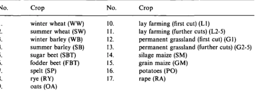
The analysis of the crop yield variations was carried out with Swiss national mean yield data from 1949 to 1986, which is based on data records of individual farmers throughout the country. All crops included in the analysis are shown in Table 1.

A time series data of the yield of each crop was used to determine the yield variations induced by the weather. Hattenschwiler (1984), who built a national crop yield simulation model based on national mean yield data from 1949 to 1979, showed that crop yield determining factors like fertilisa-tion (nitrogen, phosphor and potassium) and plant protecfertilisa-tion agents almost monotonously increased over the observed period. Other yield determining factors like technical progress, cultivation improvements and soil conditions were assumed to increase monotonously over the observed time. Since the weather was the only stochastic yield determining factor, it was possible to

Table 1. Crops included in the analysis No. 1. 2. 3. 4. 5. 6. 7. 8. 9. Crop winter wheat (WW) summer wheat (SW) winter barley (WB) summer barley (SB) sugar beet (SBT) fodder beet (FBT) spelt (SP) rye (RY) oats (OA) No. 10. 11. 12. 13. 14. 15. 16. 17. Crop

lay farming (first cut) (LI) lay farming (further cuts) (L2-5) permanent grassland (first cut) (Gl) permanent grassland (further cuts) (G2-5) silage maize (SM)

grain maize (GM) potatoes (PO) rape (RA)

include all 'monotonically' increasing factors in a time variable (t). Thus, the crop yield (y) can be written as a function of t

y=f(t) + e (i)

where the residuals e are interpreted as the yield variations induced by the weather. The function f(t) was estimated by OLS regression technique and represents the trend. The assumption that all noise is denned as weather-induced yield variations seems heroic at first glance. Hattenschwiler (1984), however, proved that fertilisation and plant protection agents are not signifi-cant exogenous variables that can be used to explain the residuals of the trend functions. Thus, it is not possible to split the noise into weather-induced and production-weather-induced yield variations.

The obtained residuals of all trend functions represent a multivariate distribution, where the corresponding density function is unknown. Thus, it was not possible to simulate straightforwardly with the help of the inverse multivariate distribution function. The only way to model the multivariate distribution was to draw on partial information about the multivariate distribution. Therefore, the correlation matrix of the residuals and the mar-ginal distribution of the residuals of each single crop were considered to exhibit some 'details' of the multivariate distribution. To show the linear relationships between the weather-induced yield variations of the various crops, the simple correlation coefficient (r), of the residuals of all 17 trend functions was calculated (see Table 2).

The question of the utilisation of aggregate data as opposed to farm-level data needs to be addressed as well. Before it is possible to advance to this point, however, a few fundamental aspects of the ERM have to be outlined. The discussion about aggregate data versus farm-level data has therefore been deferred to the end of section 2.1.5.

2.1.2. Basis crops. In this section, the core of the ERM will be introduced.

Table 2. The correlation matrix of the weather-induced yield variations for all 17 crops 01 LI G2-5 L2-5 GM SM FBT SBT RA PO OA SP WB RY SB SW WW Cl 0.821 0.343 0.408 0.013 -0.064 0.079 0.025 0.087 -0.048 -0.039 0.057 0275 0.140 0.022 -0.029 LI 0.312 0.443 10.0751 0.007 •0.024 -0.041 0.004 [-0.0281 -0.104 -0.070 0.165 0.033 -0.047 0.008 0210 1 0.1351 G2-5 0.921 0.152 0285 0.193 0212 0.097 0289 0.060 -0272 -0.022 -0.164 -0.052 -0.138 -0.152 L2-5 0.123 0.151 0.146 0.177 0.090 0243 0.110 -0245 0.000 -0.132 -0.055 -0.023 •0.100 CM 0.509 0.401 0.384 0.117 1 0.2781 -0.051 0.148 0.108 0.108 0.069 0.166 150521 SM 0.458 0.401 -0.128 0.351 -0.144 -0.094 -0.141 -0.181 -0.019 •0.102 -0.174 FBT 0.837 0.156 0.381 0.061 0.195 0225 0.235 0235 0.140 0206 SBT 0235 0.460 0.061 0.138 0207 0.169 0209 0.112 0.189 RA 0.345 0.412 0.401 0.513 0.538 0.448 0.462 PO 0.466 0.125 0.140 0239 0.424 0.370 0.591 102161 OA 0.597 0.459 0.565 0.796 0.663 0.543 SP 0.817 0.795 0.714 0.683 0.761 WB 0.783 RY 0.653 0.737 SB 0.577 0.725 0.7«t SW 0.798 0.165 0.742 0.717 WW

With a significance level of 0.1 (two-tailed) and a sample size of 38, a significant correlation results as soon as r is greater than 0.22.

magnitude of the weather-induced yield variations for one group (bundle) contains all necessary information about the prevailing weather conditions at the farm level. Then, for the second group, the magnitude of the weather-induced yield variations can be directly deduced from the first group.

A first glance at the correlation matrix shows that the weather-induced yield variations of some crops are not correlated with each other. Obviously, they obey different factual or temporal elements of the weather in each year. Therefore, the weather-induced yield variations of two uncorrelated crops are conceived as representative points of disjunctive sets of information about the weather. The weather-induced yield variations of all uncorrelated crops form the maximal, non-redundant information of the weather, as far as it is important for the yield potential. For the purpose of this work, groups of uncorrelated or very weakly correlated crops which cannot be enlarged without the formation of a subgroup with significant multicorrela-tion shall be referred to as basis or basis crops. All crops which do not belong to the basis shall be called non-basis crops. Thus, the basis crops represent the weather in the sense of 'instrumental variables'. The number of basis crops ought to be as large as possible, because each basis crop contains additional information about the weather which otherwise would not be available.

The basis crops were found with the help of a principal component analysis of the weather-induced yield variations and a successive rotation of the principal components by the varimax criterion. This analysis showed that cereals loaded on the first component, grain maize, silage maize, fodder and sugar beet on the second component, lay farming and permanent grassland (first cut) on the third component and lay farming and permanent

grassland (further cuts) as well as potatoes on the fourth component. The first four components have eigenvalues before rotating greater than one and they explain 75% of the variance of the weather-induced yield variations of all 17 crops, while the other 14 components are negligible because their loadings are low and their eigenvalues before rotating are less than one.

Most of the different crops loading on one particular component are highly correlated. The high linear dependency among these crops suggests that there is a strong redundancy of information as far as the weather is concerned. At first instance one might consider the crops with the highest loading on a particular component as a criterion for the selection of the basis crops. But it should also be kept in mind that the crops to be selected ought to be uncorrelated and that the cultivation of these crops should be widespread in Switzerland. The non-correlation is a prerequisite as far as the concept of the basis crops is concerned and it facilitates the simultaneous simulation of the basis crops, whereas the widespread cultivation of these crops is important for the accurate specification of the weather-induced yield distributions of the basis crops by the farmer.

Considering only different sets of basis crops where the single crops are cultivated throughout the country, the set with the lowest pairwise linear dependency of the basis crops was selected. The appropriate test for this selection procedure is based on Holm's principle (Holm, 1979; see also the Appendix, part I). It refers to the simple correlation coefficient (r) and allows a multiple valuation of the pairwise linear dependency of the basis crops. The overall type I error is controlled by one specified significance level. The application of this test results in the four basis crops: winter wheat, grain

maize, potatoes and lay farming (first cut). This set of basis crops is pairwise

linear-independent. The simple correlation coefficient, however, showed that potatoes and grain maize are significantly correlated. The low correlation between these two crops was taken into account for the simulation of the basis crops.

To overcome the shortcoming of the simple correlation coefficient to detect only linear relationships, the weather-induced yield variations of the selected basis crops were plotted against each other. These plots clearly indicated that it was possible to rule out non-linear relationships among the basis crops. Thus, it was confirmed that the distributions of three basis crops are not only uncorrelated, but also stochastically independent of each other and constitute a disjunctive set of information about the weather.

2.1.3. Simulation of the basis crops. After having established the idea

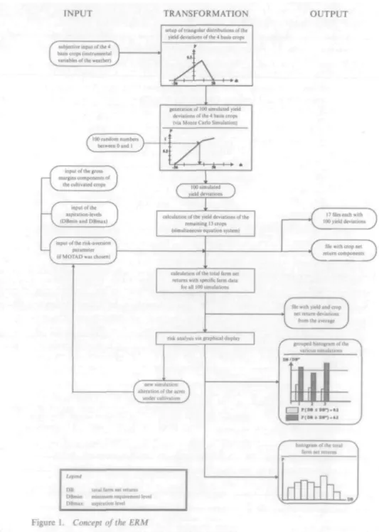
about basis crops it is possible now to return to the first objective of the ERM - the simulation of the weather-induced yield variations at the farm level. The two sections that follow describe how the concept of the basis crops can be used for the achievement of this objective.2 Figure 1 illustrates a graphical summary of the two following sections and of the risk analysis

INPUT TRANSFORMATION

f lubjccme input oflhc4 A

I bans crops (instrumental J— \ ^ variables of the weather)J

letup of truoguUr distributions of the yield deviations of ihe 4 bast* crop*

C

input of (he gross ^

margin* component* of I

the cultivated crops J

inpui of the

upu-stion-lcvcK (DBmmandDBmail

input of the mk-uvcruon \ parameter I— (if M O T A D was chosen) J

generation of 100 Simula led yield deviation* of the 4 batti crop* (via Monte Carlo Simulation)

(

1

calculation of ihc yield deviations of the remaining 13 crops (simultaneous equation system)

calculation of the total farm net returns with specific farm data

OUTPUT

(

(

UtrnJ

D B DBmn DBm.,

total fwm net fetunu aipintion level

model as well. As such it can be used as a reference for the subsequent parts of the paper. It is important to note that the preceding sections dealt exclusively with weather-induced yield variations based on national data, whereas the following sections are solely concerned with the simulation of weather-induced yield variations at farm level.

While setting up the ERM, the basis crops were selected on the grounds of national data. The underlying concept of the basis crops is now employed within the ERM to help fulfil the farm-level data requirement. This permits each farmer to specify subjectively the distribution of the crop yields of each basis crop according to his farm-specific situation. These specifications con-tain the necessary information about the farm-specific weather conditions, thus making it possible to switch from 'national data' to 'farm data'. To assess the importance of the concept of the basis crops, recall the results of the principal component analysis of the weather-induced yield variations. Only four components have an eigenvalue greater than one and they explain 75% of the total variation of the weather-induced yield variations. This reveals the high data redundancy of the weather-induced yield variations of all crops. It further suggests that the farmer's specification of the weather-induced yield variations of the basis crops covers the weather-weather-induced yield variations of all crops to a considerable extent.

As established earlier on, the weather-induced yield variations of three basis crops are stochastically independent of each other. This allows the simulation of the weather-induced yield variations of these basis crops independently, whereas the slight correlation between potatoes and grain maize has to be considered by an adequate transformation of the uniformly distributed random number used for the simulation of grain maize (for details of the so-called uniform method see the Appendix, part II, or refer to Tenenbein and Gargano, 1979; Goetz, 1991). For the actual simulation process the triangular distribution was preferred to other distributions on grounds of the three following reasons: (1) it is truncated, (2) it allows symmetric and asymmetric forms and (3) the parameters can easily be understood and specified by farmers.3 The farmer's specification of the triangular distributions for the basis crops makes it possible to simulate the weather-induced yield variations farm specifically.

This study did not explicitly examine how farmers deal with the task of encoding the probabilities, that is, specifying the parameters of the triangular distribution. Numerous studies (e.g. Tversky and Kahneman, 1982; Hogarth, 1980; von Winterfeldt and Edwards, 1986) state that severe biases and distortions are a frequent phenomenon in the process of the elicitation of subjective probabilities. To clarify the discussion Smidts (1990) notes what is meant by biases in contrast to distortions. Biases are conscious or subcon-scious discrepancies between the subject's response and an accurate descrip-tion of his underlying knowledge, whereas distordescrip-tions are interpreted as a systematic difference between the perceived and 'objective probability'. The

different methods for the elicitation of the subjective probabilities are liable to the occurrence of specific biases. The quality of the method for the elicitation of the subjective probabilities applied in this study has not yet been analysed profoundly (to the author's best knowledge). However, several studies (Pingali and Carlson, 1985; Huijsman, 1986) employing the farmer's specification of the parameters of a triangular distribution have been con-ducted. Huijsman reports that farmers had no difficulties in specifying the minimum or maximum value of the triangular distribution as opposed to the specification of the modal value. Thus the ERM gives preference to the average yield over the mode since it is suggested that the farmer is more familiar with the former. In particular, the farmer is being asked for the highest (h), lowest (/) and average (a) yield he expects as a result of weather variations over ten years. The mode (m), however, was required for the numeric simulation. The relevant formula for its calculation is as follows (Hartung, 1987: 195)

m = 3a-h-l (2)

To obtain the yield variations of the basis crops induced by the weather, the average yield was subtracted from the three parameter values of the triangular distribution for each basis crop. These values of the triangular distribution, 'centred' upon zero, were then used for the simulation. When the farmer specifies the parameters of the triangular distribution he will probably make use of his knowledge of former harvests at his farm. It may well be that his subjective information about former crop yield data for particular crops is systematically different from the objective correct crop yield data. Hence his subjective specification will be systematically distorted. This source of systematic distortion, however, is eliminated since it is the range between the parameters and not their magnitudes that now matters. Yet, unsystematic distortions still remain (see also section 2.1.5).

In some regions of Switzerland silage maize is often cultivated instead of grain maize, making it impossible for the farmers in these regions to specify the parameters of the triangular distribution of grain maize. In this case the ERM allows the farmer to choose silage maize as a basis crop and to specify the corresponding parameters of the triangular distribution of silage maize. Farmers having problems specifying the parameters of the triangular distri-bution for lay farming (first cut) or for silage maize are able to call for support within the ERM. The programme supplies the user with the volu-metric weights of various bale types and with information about the space which a dt. of hay or silage maize requires for its storing, depending on its dry-matter content. In order to enable the ERM to adjust the farmer's specification of the triangular distribution of lay farming to lay farming with four cuts, the programme additionally requests the farmer to state the number of times he cuts his grass per year.

size= 100) was done with the inverse of the respective triangular density distribution function F{X)~l (Monte Carlo Simulation).

(3) m-l X =

I + JX'ih-lXm-l), X' <

where A" is a uniformly distributed random number in the interval [0, 1], and X the simulated value of the weather-induced yield variation.

2.1.4. Calculation of the non-basis crops. The question that arises now is

how to simulate or calculate the weather-induced yield variations of the remaining non-basis crops at the farm level. It is certainly not possible to use the previously estimated correlation matrix (Table 2), since it implies the non-acceptable assumption of a multivariate normal distribution of the weather-induced yield variations (refer to section 1). For the calculation of the weather-induced yield variations of the non-basis crops (snon.basis) it is

of great help to recall: first, that the weather-induced yield variations of the basis crops (sbasis) are independent of each other; and second, that the

weather-induced yield variations of the non-basis crops correlate with the weather-induced yield variations of the basis crops and with each other. One can thus conclude that the weather-induced yield variations of the basis crops are explanatory for the corresponding weather-induced yield variations of the non-basis crops:

Einon-basi,=f(£basis) + Vi (5)

The index i stands for one particular non-basis crop and runs from 1 to 13. Once the weather-induced yield variations of a non-basis crop are explained by those of one or several basis crops, the particular weather-induced yield variations of this crop can also be used to explain those of the remaining non-basis crops.

The above-described sequence of explanation of the weather-induced yield variations of the non-basis crops can be used to derive a recursive simulta-neous equation system. Further proving the condition, Corr^,; ui + 1) = 0 makes it admissible to estimate the equation system by the OLS regression technique (Koutsoyiannis, 1979). Two simultaneous equation systems were estimated, one with grain maize and the other with silage maize belonging to the basis. For a clear understanding of the crop yield simulation model it is relevant to mention that the parameters of the recursive simultaneous equation system were estimated with national data. The simulated weather-induced yield variations of the basis crops serve as an input for the recursive simultaneous equation system and thus allow the calculation of the

weather-induced yield variations of the non-basis crops, where the residuals vt of

equation 5 had to be simulated. Assuming normally distributed residuals, the mean and standard deviations were calculated and used for the simula-tion which was done within the ±3a limits. A truncated distribusimula-tion was chosen for two reasons: firstly, because the residuals cannot be infinitely small or large, and secondly because this modelling is in line with the modelling of the basis crops.

2.1.5. Validation of the crop yield simulation model. Finally, the quality of

the simulation model was examined with the help of statistical tests. A first test compared the correlation matrix calculated from the observed weather-induced yield variations of all crops (1949-1986) with a correlation matrix calculated from simulated weather-induced yield variations (Fischer's Z-Transformation, Gauss-Sample Test; Hartung, 1987: 548). Since this test only compares two corresponding correlation coefficients of the respective correlation matrices, it does not take into consideration the multivariate aspect of the comparison. To take care of this shortcoming, a particular test based on the maximum root criterion of S. N. Roy (1957) has been conducted (Krishnaiah et al., 1980; see also the Appendix, part III). Two further tests evaluated the conformity between the marginal distribution of the observed weather-induced yield variations of each crop with a marginal distribution of simulated weather-induced yield variations (Mann-Whitney Test [Har-tung, 1987: 513]; Chi-Square Homogeneity Test for loglinear r x s-tables, [Hartung, 1987: 433]). Whereas the Mann-Whitney Test evaluates primarily the location of the distribution, the Chi-Square Homogeneity Test focusses on the form of the distribution. Recognizing the imperfection of the model, a sensitivity analysis of the simulation model in respect to the farmer's specification of the crop yield estimates was carried out. The input data for the basis crop was systematically varied from the originally observed data in the statistical tests in order to make an assessment of the previously so-called unsystematic distortions of the parameters of the subjectively specified triangular distributions and their effect on the results of the simulation model.4 In view of space constraint, only a condensed presentation of the results of the statistical tests will follow (for a detailed presentation see Goetz, 1991). The 200 Gauss-Sample Tests5 that were conducted showed that it is not possible to reject the hypothesis (Ho) that the correlation

matrix calculated from the observed weather-induced yield variations is equivalent to a correlation matrix calculated from simulated weather-induced yield variations. The test based on the maximum root criterion of S. N. Roy supported these previous results. None of the results obtained allowed the rejection of the hypothesis (HQ) that the 'observed covariance

matrix' and a 'simulated covariance matrix' are equivalent. The same results with respect to the hypothesis (Ho) (the marginal distribution of the observed

weather-induced yield variations of one crop is equivalent to a marginal distribution of the simulated weather-induced yield variations of this crop)

hold completely for the 1122 conducted Mann-Whitney Tests.6 105 out of 1122 conducted Chi-Square Homogeneity Tests could not support the hypothesis (Ho) which is equivalent to the tf0-hypothesis of the Mann-Whitney Test. This occurred particularly in the case of spelt where the Ho

-hypothesis was rejected 47 times. Overall it was possible to accept the simulation model on grounds of statistical tests. Yet, the results indicated that the variation of the input data for the basis crops did not have a 'significant' influence on the 'quality' of the performance of the simulation model.

By now it is time to return to the question of the utilisation of national data as opposed to cantonal or farm-level data. On the one hand, broadly aggregated data inevitably means a loss of information due to aggregation. Use of cantonal data, on the other hand, implies a high redundancy of the data caused by the topographic similarity and the close range of particular cantons. Hattenschwiler (1984: appendix III-2) examined the question of national versus cantonal data in detail and found that the loss of information through the use of national data was quite minimal. He showed in particular that the non-linear stochastic dependencies between the weather-induced yield variations for each crop, the corresponding correlation matrix (linear stochastic dependencies) and the simultaneous equation system for the calculation of the nonbasis crops for both data sets national and cantonal -do not differ significantly from each other. This leads to the hypothesis that the interdependencies of the weather-induced yield variations do not vary significantly within Switzerland (space invariance). This is not intended to say that weather-induced yield variations at farm level do not vary within Switzerland, but that their interdependencies are fairly stable.

Weather-induced yield variations based on cantonal data, however, are still not representative for weather-induced yield variations at farm level. In moving from aggregate data (national or cantonal) to farm-level data, two concepts are employed. First is the concept of the basis crops where the farmer's specification of the triangular distribution of the basis crops covers the weather-induced yield variations of all crops to a substantial extent. The second concept entails utilising the hypothesis of space invariance between the weather-induced yield variations of the basis crops and the non-basis crops. This allows the calculation of the weather-induced yield variations of the non-basis crops at the farm level with the help of the basis crops.

3. Application of the crop yield simulation and risk analysis model

The simulation of the weather-induced yield variations itself is not of much help to the farmer. The information of the simulation model needs to be condensed in order to make it possible to compare the effects of different crop-rotation plans on the farm net returns (risk analysis). In this section,

0.50 0.40 0.30 0.20 0.10 0.00

Histogram of the farm net returns

expected value = 145725.07 standard deviation =14453.10

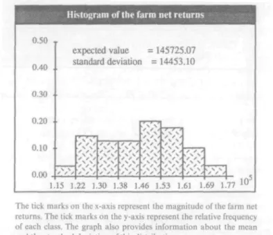
1.15 1.22 1.30 1.38 1.46 1.53 1.61 1.69 1.77 The tick marks on the x-axis represent the magnitude of the farm net returns. The tick marks on the y-axis represent the relative frequency of each class. The graph also provides information about the mean ;ind the standard deviation of this distribution.

Figure 2. Histogram of the farm net returns for the initial crop-rotation plan of the analysed farm

the features of the risk analysis model as well as the results of a risk analysis that was carried out for a particular farm are presented. This farm is specialised in crop production with 30 hectares of cultivated land and a labour force of 2.5 men. The corresponding linear programming model is composed of 23 variables and 21 restrictions.

The simulated weather-induced crop yield variations of this particular farm were produced with usual values for the parameters of the triangular distribution of the basis crops. The simulated yield variations together with the farmer's specification of a crop-rotation plan (LP-solution or actual crop-rotation plan), the average yields, the prices, the costs, etc. (crop net return components), allow the computation of the weather-induced distribu-tion of the farm net returns for a particular crop-rotadistribu-tion plan. Figure 2 illustrates the distribution of the farm net returns for the optimal solution of the linear programming model of this farm.7 Users of the ERM who intend reducing the risk8 associated with particular crop-rotation plans have two options open to them. These include the MOTAD-model9 (Hazell and Norton, 1986) and the heuristic approach.

If a MOTAD-model is chosen, a representative sample of the 'simulated data' adequate to the distribution of the farm net returns is drawn. This sample based on 20% of the 'simulated data' makes up the expected value of (a) the net return of each cash crop,

and 20 deviations of

(c) the net return of each cash crop from the corresponding expected value, (d) the yield of each forage crop from the corresponding expected value.

With this information, the sample could then be passed on to a linear programming model to add 'restrictions' in the sense of MOTAD. The user also has the option of including the forage crops in the risk analysis. If he decides to include it, he needs to monetarise the deviations of the yields of each forage crop, and add this information to the linear programming model in the form of restrictions in line with the 'penalty cost aproach' (Hanf and Mueller, 1979). It is important to note that the ERM supplies the necessary data to convert an ordinary linear programming model (maximisation of the expected farm returns) into a MOTAD-model, but the risk analysis model of the ERM does not include any linear programming technique. The data for a MOTAD-model produced by the ERM has to be added to an ordinary linear programming model by the user. The ERM can then be used to produce a distribution of the farm net returns based on a crop-rotation plan that results from the optimisation of a MOTAD-model.

The choice of a MOTAD-model implies the specification of a risk-aversion parameter Q. In this study the risk-aversion parameter is used to produce risk-efficient crop-rotation plans. By varying the risk-aversion parameter for example from 0 to 2.5, different crop-rotation plans can be obtained through the optimisation of the MOTAD-model. The values of the risk-aversion parameter represent initially a risk-neutral farmer who becomes more and more risk-averse as the risk-aversion parameter increases. The corresponding distributions of the farm net returns can then be calculated with the help of the ERM. Whenever the user calculates this distribution again he only needs to alter the specification for the hectares planted with a specific crop. All other information is handled by the programme.

Figure 3 presents the results of a risk analysis for the analysed farm. A comparison of Figures 2 and 3 reveals that the expected value of the farm net returns (x) decreased from 145,725 SFrs. to 138,086 SFrs. and the stan-dard deviation of the farm net returns (s) from 14,453 SFrs. to 10,040 SFrs.10 The coefficient of variation (s/x) dropped from 0.1 to 0.07. The activities of the arable farm sector altered substantially for the farm, suggesting its response to weather-induced yield variations. A further reduction of the risk measured as the standard deviation of the farm net returns was, however, not feasible - the crop-rotation plan remained unchanged (see Table 3).

The ERM offers its users the possibility of applying graphical presentations to contrast these different crop-rotation plans with respect to the tails of the distribution of the farm net returns - the lower and upper quintils. Figure 4 is used to provide an example of such a graphical comparison of the risk analysis of the analysed farm.11

Quite evident from the diagram are:

Histouram <»l the larin iitl upturns 0.40 , 0.30 • 0 20 • 0.10 • O.OO -expected value standard deviation y / ' y y • y y • y y * y y • y y • y y = 138113.37 = 10012.82 f y y ' y y * y y f y y * y y * y y * y y 1.15 1.21 1.27 1.32 1.38 1.44 1.49 1.55 1.61 105 Figure 3.

The tick marks on the x-axis represent the magnitude of the farm net returns. The tick marks on the y-axis represent the relative frequency of each class.

Histogram of the farm net returns for the crop-rotation plan resulting from the MOTAD-model for the analysed farm (Q = 2.5)

and

(b) the farm net returns forming the lower and upper quintils.

The output of Figures 2, 3 and 4 should enable the farmer to decide on one specific crop-rotation plan that matches his attitude towards risk. Figures 2 and 3 give him information about the expected value, the standard deviation and the distribution of the farm net returns, whereas Figure 4 supplies him with the particular interesting information of the lower and upper quintil.

Table 3. Changes of the crop-rotation plan Risk-aversion parameter 0.0 0.5 1.0 1.5 2.0 2.5 3.0 3.5 4.0 4.5 5.0 PO 6.25 6.25 6.25 6.25 3.85 3.85 3.85 3.85 3.85 3.85 3.85 RA 2.0 2.0 2.0 2.0 0.15 0.0 0.0 0.0 0.0 0.0 0.0 GM 5.0 5.0 5.0 5.0 5.0 5.0 5.0 5.0 5.0 5.0 5.0 WW 0.0 0.0 0.0 1.28 0.15 0.15 0.15 0.15 0.15 0.15 0.15 SW 3.75 0.0 0.0 0.0 0.0 0.0 0.0 0.0 0.0 0.0 0.0 WB 2.0 5.75 5.75 4.47 10.0 10.0 10.0 10.0 10.0 10.0 10.0 SBT 2.4 2.4 2.4 2.4 2.4 2.4 2.4 2.4 2.4 2.4 2.4 L1/L2-5 3.6 3.6 3.6 3.6 3.6 3.6 3.6 3.6 3.6 3.6 3.6 GI/G2-5 5.0 5.0 5.0 5.0 5.0 5.0 5.0 5.0 5.0 5.0 5.0

tiimi plans and their associated risk

0.00 1.00 2.00 2.50

risk-aversion parameter risk parameters for the different farm plans The personal aspiration-levels for the farm net returns are: — - 110000.00 145000.00

The farm net returns will in a maximum of two out of ten years fall below this value

The farm net returns will in a maximum of two out of ten vears exceed this value

The tick marks on the x-axis represent the magnitude of the risk-aversion parame-ter. The tick marks on the y-axis represent the farm net returns

Figure 4. Comparison of the different crop-rotation plans with respect to their lower and upper quintil of the farm net returns and to the user s minimum requirement and aspiration levels

While deciding on one particular crop-rotation plan it is necessary to con-sider all three diagrams together to get all the information available from the ERM. To look only at the upper and lower quintil of the farm net returns for instance could easily be misleading for the choice of a risk-efficient crop-rotation plan.

In case a heuristic approach is opted for, the user reduces the risk associ-ated with an initial crop-rotation plan heuristically by altering the initial crop-rotation plan. While Figures 2 and 3 remain the same, the risk-aversion parameter in Figure 4 would be replaced by the successive numbers of the different crop-rotation plans that the user created. Thus, the graphics allow the user to assess the effects of the alterations of the crop-rotation plan on the distribution of the farm net returns and to decide which crop-rotation plan is most suitable for him.

4. Summary and conclusions

This paper has examined the current approaches for solving the problem of allocating land on a single farm to a mix of crops under uncertainty, where

the weather-induced yield variations were interpreted as the major source of uncertainty for the farmer in Switzerland. The proposed model for solving this problem does not, as opposed to previous models, employ a utility function and one particular decision rule (optionally), nor does it rely on recorded crop yield data related to the past as an input from the user. Instead, the model provides each individual user with several options. This opens up the possibility of adopting the model to the user's needs and thus strengthens its empirical utilisation. The detailed specification of the crop yield simulation and risk-analysis model (ERM) have made it possible to build a PC-based programme that can easily be operated by farmers or extension personnel.

The ERM and a MOTAD-model were used in 'farm planning' of an arable farm to illustrate the empirical use of the ERM. With an increase of the risk-aversion parameter of the MOTAD-model, the original crop-rotation plan changed substantially. The ERM showed that the changes in the crop-rotation plan led to a decrease in the expected value and the associated risk in terms of the standard deviation of the farm net returns. It is possible for the farmer to reduce the standard deviation of the farm net returns by 30%; on the other hand, he has to put up with a 5% decrease in the expected value. Since the ERM does not require recorded crop yield data it is readily applicable. It has been designed to help extension officers in their efforts to produce qualified decision support for farmers. This paper gives an example of the application focussing on one particular problem. In practice the ERM may also be useful to simulate the distribution of the farm net returns for a given crop-rotation plan in order to determine cash flow planning. Another possible area of application is in production analysis. Given a deterministic production function the utilisation of the ERM may improve the closeness of the analysis to reality by supplying the simulated weather-induced yield variations. For the same reason, the ERM may be useful in national sector modelling, provided the sector model is based on farm sample models (Hanf, 1989).

The crop yield simulation model was statistically validated and found to be robust in respect to changes in the farmers' specification of the yields for the basis crops. The ERM was applied to a particular problem to demon-strate its use under a practical setting. It is presently not possible to assess the ERM as regards its acceptance and usefulness by farmers and extension personnel since it has just been released. An evaluation of the ERM at a later point in time, considering these aspects, should also include an examina-tion of the underlying hypothesis of the invariance with respect to space between the weather-induced yield variations. This hypothesis resulted from a statistical analysis of the observed weather-induced yield variations. Thus it is not possible to validate this hypothesis statistically with the present and already utilised data. A statistical validation of this hypothesis as such has to be deferred to a later point in time when enough new data are available.

Appendix

(I)

Holm's multiple test of pairwise linear independency of p samples with the length (n) is based on the simple correlation coefficient. For all pairs of the samples the simple correlation coefficient (rik), 1 < i < fc < p, is calculated and the p(p — l)/2 test statistic

(6) is sorted in an ascending order.

Ri,k, ^ Ri2k2 ^ Ki3k3 ^ • " S:Rip(P-1)/2*p(p-l)/2 W

T h e n successively for m = 1 ••• p{p — l)/2 the following inequality is verified:

Rimkm < tn- 2 ; l - a / ( p ( p - l ) + 2 - 2 m ) (8)

As soon as this inequality holds for one m the first time the true correlation coefficients Pi,*, •" Pim-i*»,-i a r e significantly different from zero at the significance level a, all remaining

correlation coefficients are not significantly different from zero. (II)

The random number V within the interval [0, 1] is used for the simulation of potatoes. In order to simulate grain maize with a specific correlation coefficient with respect to potatoes, the following transformations of V and V were done:

1. It is assumed that there are two independent uniformly distributed random numbers U' and V within the interval [0, 1],

2. U = U' and V=cU' + (1 - c)V for a fixed value of c. Bivariate distributions with corre-sponding correlation coefficients can be produced by specifying c.

3. X' = U V = V2 /26(1 - b) (O^K^fc) (9) = 2V~b/2(l-b) (b<V^l-b) (10) = l - ( l - K )2/ 2 f e ( l - f c ) ( l - f o < K < M ) (11) where b = min(c, 1 — c) 4. X = Fr'(A")and y = F f ' ( y ' )

F f ' ( ) represents the inverse distribution function of both crops, where X and Y stand for the respective weather-induced yield variations of potatoes and grain maize.

(Ill)

Ci and C2 are sample covariance matrices of two p-variate normal samples of size n; in the

usual unbiased form. Then the matrix F = C, C J ' is said to have the multivariate F-distribution. /:, <?.2< ••• <).p denote the characteristic roots of F; these are positive and distinct with probability 1. Roy's test for Ho: Ct = C2 is based on the fact that Ct = C2 exactly if the largest

and the smallest characteristic roots of C, C J ' are both unity, and the Ho hypothesis is rejected

if /., is smaller than some critical value c,, or /.„ is larger than some critical value cp (Pillai

Notes

1. Ertragssimulations- und Risikoanalysemodell (crop yield simulation and risk analysis model); this programme runs on personal computers (PC) based on DOS and can be obtained from the author for SFrs. 49,-.

2. It would certainly be possible to use the first four principal components for the simulation of the weather-induced yield variations at farm level. However, these four linear-indepen-dent components cannot be utilized since the principal component analysis is based on national data. To produce farm-level data for the simulation process the farmer's subjective specification of the weather-induced yield distribution for all crops loading on the first four components is needed. Yet, it is suggested that this approach would be very tedious under practical conditions, and above all only very few farmers will be able to specify completely the weather-induced yield distribution for all crops loading on the first four components. An incisive reduction of the numbers of crops where the farmer has to specify the weather-induced yield distribution seems to be inevitable. These considerations prop up the concept of the basis crops as a theoretically appropriate and very practical approach for producing farm-level data.

3. Since the study considered only the triangular distribution it is not in a position to report on the performance of other distributions.

4. A more profound sensitivity analysis of the farmer's specification of the parameter of the triangular distributions would be based on the assumption of a specific distribution of the error term (misspecification). Let the error term be additive and normally distributed with an expected value of zero and a standard deviation <rr; [iV(0, <7,)]. Thus, equation 4 can be

written as: ) - / - JV(O, <7, ))(m + N(0, <r2) - / - N(0, CT, )), m + N(0,ai)-l-N{0,ai) h + N(0, <r3) - y i - X'(h + N(0, CT3) - / - JV(O, IT, )){h + N(0, <r3) - m - N(0, ., „ , m + Ar(0<r)-/-Af(0 (12)

This equation allows one to simulate the basis crops as a function of the three parameters (/, m, h), the uniformly distributed random number X' and the parameter a,. In order to evaluate the effects of a misspecification, the parameter <J, must be analysed. Therefore, a norm in the Sf1

needs to be defined. A transformed euclidean distance is proposed here.

\a\\, = s/l'2a\ + m-1a\ + h'2a\ (13)

Please note that if /, m, h were set to 1 the normal euclidean distance would result.

This procedure makes it possible to determine all CT, attributed to a particular level of misspeci-fication [la II,. For instance let Hall, = 0.1; then all points on the surface of a sphere will satisfy equation (13). The level of misspecification, e.g. jit7||, = 0.1, can be interpreted in terms of the coefficient of variation. A sample size n, with permissible triples of (u,, a2, <r3), can be used for

the simulation of the basis crops [equation (12)]. These values serve as an input for the simulta-neous equation system. Subsequently the distribution of the farm net returns can be calculated. The obtained distribution should be compared statistically with the distribution of the farm net returns with no error terms to evaluate the effects of a misspecification.

Although this kind of sensitivity analysis permits one to assess the simulation model quite well, it is suggested here that it would not benefit directly the user of the ERM. This is in part so because the farmer specifies the parameter of the triangular distribution to the best of his knowledge and therefore is not able to judge whether he misspecified and to what extent.

Without any information about his possible misspecification he cannot make use of a sensitivity analysis that quantifies the effects of his misspecification on the distribution of the farm net returns. Moreover, the determination of the size of the misspecification is too complex under a practical setting. Considering these facts and given the scope of this particular study, the author did not attempt to quantify the effects of a misspecification of the parameters on the distribution of the farm net returns. It was rather statistically tested whether the simulated distributions of all crops considered in this study under the assumption of correctly and incorrectly specified input data are equivalent to the observed distributions. In other words the 'quality' of the simulation model in cases of misspecified parameters was evaluated and not its quantitative effects.

5. The input data for the crop yield simulation model was varied 50 times, each with grain maize and with silage maize as a basis crop. Thus, 100 correlation matrices stem from these calculations. Furthermore, the model was tested with a sample size of 300 as well, which resulted in another 100 correlation matrices.

6. Since the results of the Gauss Sample Tests showed no 'significant' differences between the crop yield simulation models with the different sample sizes, the subsequent Roy, Mann-Whitney and Chi-Square Homogeneity Tests were only conducted with the simulated yields of one sample size. To further limit the data being processed, only 33 variations of the input data for both of the crop yield simulation models (grain and silage maize) were considered for the last two tests.

[(17 (crops)*33 (variations)*2 (type of model) = 1122 tests].

7. To give the reader a realistic introduction to the ERM the actual output of the programme has been chosen for Figures 2, 3 and 4.

8. The term risk refers to the shape of the distribution of the farm net returns. 9. MOTAD stands for Minimum of Total Absolute Deviation.

10. The reader has probably noticed that the ranges of the bars and the overall range on the x-axis are different in Figures 2 and 3. When the ERM was programmed it was decided to scale the graphics flexibly, i.e. according to the data being processed. Otherwise with fixed ranges of the bars and fixed boundaries on the x-axis, it may well happen after a change of the crop-rotation plan, that data will not be presented because they go beyond the bound-aries, or the histrogram will not be very meaningful since most of the data may be concen-trated in one or two bars. It is recommended that a new version of the ERM should be interactive, so that the user can scale the graphics to his needs. At present the user of the ERM could also employ an ordinary statistical package to produce these graphics accord-ing to his needs by makaccord-ing use of the files that the ERM puts onto the disk of his personal computer.

11. As one of the reviewers pointed out, a high-low graphic would probably be easier to grasp for the user of the ERM.

References

Arrow, Kenneth J. (1971). Essays of the Theory of Risk Bearing. Amsterdam: North-Holland. Barry, Peter J. (1984). The setting. In Peter J. Barry (ed.), Risk Management in Agriculture. Ames:

Iowa State University Press.

Binswanger, H. P. (1980). Attitudes towards risk: experimental measurement of rural India. American Journal of Agricultural Economics 62(3): 395-407.

Buccola, Steven T. (1986). Testing for nonnormality in farm net returns. American Journal of Agricultural Economics 68(2): 334-343.

Collender, Robert N. and Chalfant, James A. (1986). An alternative approach to decisions under uncertainty using the empirical moment-generating function. American Journal of Agricultural Economics 68(4): 721-731.

Collender, Robert N. and Zilberman, David (1985). Land allocation under uncertainty for alternative specifications of return distributions. American Journal of Agricultural Economics 67(4): 779-786.

Day, Richard H. (1965). Probability distributions of field crops. Journal of Farm Economics 47:713-741.

Frankenberg, Peter (1984). Ahnlichkeitsstrukturen von Ernteertrag und Witterung in der Bundesrepublik Deutschland. Wiesbaden: Steiner.

Freund, C. J. (1956). Introduction of risk into a programming model. Econometrica 24: 253-263. Goetz, R. U. (1991). Der Einflufi witterungsbedingter Ertragsschwankungen auf die

landwirtschaftliche Betriebsplanung. Kiel: Wissenschaftsverlag Vauk.

Hamal, K. B. and Anderson, J. R. (1982). A note on decreasing absolute risk-aversion among farmers in Nepal. Australian Journal of Agricultural Economics 26: 220-225.

Hanf, C.-H. (1989). Agricultural Sector Analysis by Linear Programming - Approaches, Problems and Experiences. Kiel: Wissenschaftsverlag Vauk.

Hanf, C.-H. and Miiller, R. A. E. (1979). Linear risk programming in supply response analysis. European Review of Agricultural Economics 6: 435-452.

Hartung, J. (1987). Statistik: Lehrbuch der angewandten Statistik, 6th ed. Munich: Oldenbourg. Hattenschwiler, Pius (1984). Risikoanalyse zur Ernahrungsplanung. Unpublished Ph.D. thesis,

ETH-Zurich.

Hazell, Peter B. R. and Norton, Roger D. (1986). Mathematical Programming for Economic Analysis in Agriculture. New York: Macmillan.

Hershey, J. C , Kunreuther, H. and Shoemaker, P. M. (1982). Bias in assessment procedures for utility functions. Management Science 28: 936-954.

Hogarth, R. M. (1980). Judgement and Choice: The Psychology of Decision. New York: Wiley. Holm, A. (1979). A simple sequentially rejective multiple test procedure. Scandinavian Journal of

Statistics 6: 65-70.

Huijsman, A. (1986). Choice and uncertainty in a semisubsistence economy. A study of decision making in a Philippine village. Unpublished Ph.D. thesis, Agricultural University Wageningen.

Jones, C. A. and Kiniry, J. R. (eds.) (1986). CERES-Maize: A Simulation of Maize Growth and Development. College Station: Texas A&M University Press.

Keeney, Ralph L. and Raiffa, Howard (1976). Decisions with Multiple Objectives: Preferences and Value Tradeoffs. New York: Wiley.

King, Robert P. and Robinson, Lindon J. (1984). Risk efficiency models. In Peter J. Barry (ed.), Risk Management in Agriculture. Ames: Iowa State University Press.

Koutsoyiannis, A. (1979). Theory of Econometrics, 2nd ed. London and Basingstoke: Macmillan. Krishnaiah, P. R., Mudholkar, G. S. and Subbaiah, P. (1980). Simultaneous test procedures for mean vectors and covariance matrices. In P. R. Krishnaiah (ed.), Analysis of Variance, New York: North-Holland.

Markowitz, H. M. (1970). Portfolio Selection: Efficient Diversification of Investment, 2nd ed. New York: Yale University Press.

Oskam, A. J. (1991). Weather indices of agricultural production in the Netherlands 1948-1989. Netherlands Journal of Agricultural Science 39(3): 149-164.

Palutikof, J. P., Wigley, T. M. L. and Lough, J. M. (1984). Seasonal climate scenarios for Europe and North America in a high-CO2 environment. Climatic Research Unit, School of

Environmental Sciences, University of East Anglia, Norwich.

Penning de Vries, F. W. T., Jansen, D. M., ten Berge, H. F. M. and Bakema, A. (1989). Simulation of Ecophysiological Processes of Growth in Several Annual Crops. Wageningen: PUDOC, Centre for Agricultural Publishing and Documentation.

Pillai, K. C. S. and Flury, Bernhard N. (1985). Upper Percentage Points of the Largest Character-istic Root of the Multivariate F-Matrix. Technical Report 17. Department of StatCharacter-istics, University of Berne.

Pingali, P. L. and Carlson, G. A. (1985). Human capital, adjustments in subjective probabilities, and the demand for pest controls. American Journal of Agricultural Economics 67: 853-861.

Pratt, J. W. (1964). Risk aversion in the small and in the large. Econometrica 32(1-2): 122-136. Roy, S. N. (1957). Some Aspects of Multivariate Analysis. New York: Wiley.

Smidts, A. (1990). Decision Making under Risk, A Study of Models and Measurement Procedures with Special Reference to the Farmer's Marketing Behaviour. Wageningen Economic Studies No. 18. Wageningen: PUDOC.

Sonka, Steven T. and Patrick, George F. (1984). Risk management and decision making in agricultural firms. In Peter J. Barry (ed.), Risk Mangement in Agriculture. Ames: Iowa State University Press.

Tenenbein, A. and Gargano, M. (1979). Simulation of bivariate distributions with given marginal distribution functions. In N. R. Adam and A. Dogramaci (ed.), Current Issues in Computer Simulation. New York: Academic Press.

Tversky, A. and Kahnemann, D. (1982). Judgement under uncertainty: heuristics and biases. In A. Tversky, D. Kahnemann and P. Slovic (eds.), Judgement under Uncertainty. New York: Cambridge University Press,

von Neumann, J. and Morgenstern, O. (1953). Theory of Games and Economic Behavior, 3rd ed. Princeton: Princeton University Press,

von Winterfeldt, D. and Edwards, W. (1986). Decision Analysis and Behavioral Research. Cambridge: Cambridge University Press.

R. U. Goetz

Swiss Federal Institute of Technology Department of Agricultural Economics Sonneggstrasse 33

8092 Zurich Switzerland