Class proximity measures—dissimilarity-based classification and display of high-dimensional data

Publisher’s version / Version de l'éditeur:

Journal of Biomedical Informatics, 44, 5, pp. 775-778, 2011-04-27

READ THESE TERMS AND CONDITIONS CAREFULLY BEFORE USING THIS WEBSITE.

https://nrc-publications.canada.ca/eng/copyright

Vous avez des questions? Nous pouvons vous aider. Pour communiquer directement avec un auteur, consultez la première page de la revue dans laquelle son article a été publié afin de trouver ses coordonnées. Si vous n’arrivez pas à les repérer, communiquez avec nous à PublicationsArchive-ArchivesPublications@nrc-cnrc.gc.ca.

Questions? Contact the NRC Publications Archive team at

PublicationsArchive-ArchivesPublications@nrc-cnrc.gc.ca. If you wish to email the authors directly, please see the first page of the publication for their contact information.

NRC Publications Archive

Archives des publications du CNRC

This publication could be one of several versions: author’s original, accepted manuscript or the publisher’s version. / La version de cette publication peut être l’une des suivantes : la version prépublication de l’auteur, la version acceptée du manuscrit ou la version de l’éditeur.

For the publisher’s version, please access the DOI link below./ Pour consulter la version de l’éditeur, utilisez le lien DOI ci-dessous.

https://doi.org/10.1016/j.jbi.2011.04.004

Access and use of this website and the material on it are subject to the Terms and Conditions set forth at Class proximity measures—dissimilarity-based classification and display of high-dimensional data

Somorjai, R. L.; Dolenko, B.; Nikulin, A.; Roberson, W.; Thiessen, N.

https://publications-cnrc.canada.ca/fra/droits

L’accès à ce site Web et l’utilisation de son contenu sont assujettis aux conditions présentées dans le site LISEZ CES CONDITIONS ATTENTIVEMENT AVANT D’UTILISER CE SITE WEB.

NRC Publications Record / Notice d'Archives des publications de CNRC: https://nrc-publications.canada.ca/eng/view/object/?id=edb234bd-d47a-4a84-8a3b-383a857545dc https://publications-cnrc.canada.ca/fra/voir/objet/?id=edb234bd-d47a-4a84-8a3b-383a857545dc

Class proximity measures

– Dissimilarity-based classification and

display of high-dimensional data

 R.L. Somorjaia

 B. Dolenkoa

 A. Nikulina

 W. Robersona

 N. Thiessenb

 a _{Institute for Biodiagnostics, National Research Council Canada, 435 Ellice} Avenue, Winnipeg, MB, Canada R3B 1Y6

 b _{Genome Sciences Centre, BC Cancer Agency, 570 West 7th Ave. – Suite 100,} Vancouver, BC, Canada V5Z 4S6

Abstract

For two-class problems, we introduce and construct mappings of high-dimensional instances into dissimilarity (distance)-based Class-Proximity Planes. The Class

Proximity Projections are extensions of our earlier relative distance plane mapping, and thus provide a more general and unified approach to the simultaneous classification and visualization of many-feature datasets. The mappings display all L-dimensional

instances in two-dimensional coordinate systems, whose two axes represent the two distances of the instances to various pre-defined proximity measures of the two classes. The Class Proximity mappings provide a variety of different perspectives of the dataset to be classified and visualized. We report and compare the classification and

visualization results obtained with various Class Proximity Projections and their

combinations on four datasets from the UCI data base, as well as on a particular high-dimensional biomedical dataset.

Keywords

Mappings; Projections; Class-proximity planes; High-dimensional data; Proximity measures; Distance/dissimilarity measures; Visualization; Classification

1. Introduction

The promise and potential of noninvasive diagnosis/prognosis of diseases and disease states is the principal reason for acquiring specific types of biomedical data (e.g., spectra or gene microarrays) from biofluids and tissues. However, such data are characterized by relatively few instances (samples) (N = O(10)–O(100)), initially in a very high-dimensional feature space, with dimensionality L = O(1000)–O(10,000). These two characteristics lead to the twin curses of dimensionality and dataset

sparsity[38]. Any analysis of such data calls for special considerations. To lift the curse

of dimensionality, the obvious, standard course of action is to carry out feature

selection/extraction/generation (this may be avoided by using kernel SVMs, but with a concomitant loss of interpretability). Many approaches are possible. A particular,

powerful version is a dissimilarity (distance)-based, dimensionality-reducing

mapping/projection from L to two dimensions (only two, because we shall consider only 2-class problems. Higher dimensional mappings are also feasible; however, in more than three dimensions the classification results cannot be visualized.) Naturally,

mapping to lower dimensions inevitably leads to information loss; hence, not all original distances can be preserved exactly. A number of projection methods, e.g., Isomap [42], Multidimensional Scaling [6], etc. attempt to minimize the projection errors for all

distances. However, as we have shown earlier for the relative distance plane (RDP) mapping [39], the exact preservation of all distances is not necessary for an

exactvisualization in some distance plane. The relative distance plane is created by any

instance’s two relative distances (two new features) to any pair of other instances, one from each class. Furthermore, the mapping appears to preserve whatever class

separation exists in the original feature space. A direct classification in this projected

distance plane is then feasible and may reveal additional, useful information about the originally high-dimensional dataset (see e.g., [41]).

Encouraged by the successes and promise of the RDP mapping, in this work we explore and extend this dissimilarity-based concept. Of course, dissimilarity/distance-based classification is not new. In fact, all nearest neighbor classifiers [9] and [11] are distance based. “Instance-based classification” is a generalization of this model-free approach, also using nearest neighbor concepts (e.g., [44]). Since the early 2000s, Duin’s group has been advocating distance-based classification, e.g., in [33], [35], [29], [30] and [34], etc. For a thorough discussion of many relevant theoretical and practical issues, see [36].

The possibility of converting L-dimensional (L arbitrary) datasets into 2-dimensional equivalents via general and adaptable distance-based mappings is very attractive and has important implications, especially for L N. The most general conceptual extension and subsequent implementation of such a mapping require selecting both a class

proximity measure π and a distance/dissimilarity measure Δ. (Note that dissimilarity is

the more general concept and does not have to be a metric.) We may create a flexible framework for both classification and visualization by generating a wide range of [π; Δ] pairs. An important extension of this mapping process is the use of class-dependent [π;

Δ] pairs, i.e., in its most general form for class 1, for class 2. An example is Regularized Discriminant Analysis, with different for the two classes [18] and [15].

Quadratic Discriminant Analysis is a special case. Other [π ; Δ ] choices are (K1, K2)-NN classifiers, K1≠ K2[19]. Paredes and Vidal introduced a class-dependent dissimilarity measure [31]. Class-dependent PCA/PLS is often used in the popular software SIMCA-P ([12]).

Here we introduce and discuss a few of the many possibilities, both for

distance/dissimilarity and class proximity measures. We implemented the majority of these in our software CPP (Class Proximity Projector, vide infra). The major goal and thrust of the paper is threefold: (a) Choose different class proximity measures (πνs) to

this Δ, compute and display the two distances d1(Z), d2(Z) of an instance Z to the chosen πν.

The article is organized as follows. In the Introduction, we already discussed the motivation for using a distance-dependent approach for both the visualization and classification of high-dimensional data. Next, we define and list the various common distance measures we may use. This is followed by the description of several possible class representations and class proximity measures. In particular, we introduce, discuss and compare four major categories for representing and positioning an instance in a Class Proximity (CP) plane. In the Results and Discussion section we first illustrate in detail, on a high-dimensional biomedical (metabolomic) dataset (1H NMR spectra of a biofluid) several feasible possibilities and processes, based on concepts of the Class Proximity Projection approach. We repeat this process for four datasets from the UCI Repository. We conclude with general observations and a summary.

1.1. Distance measures Δ

Consider a two-class dataset, and assume that the data comprise N instances in an L-dimensional feature space. Thus the original mth instance vector Z(m) has L components

, m = 1, … , N, N = N1 + N2, with Nk instances in class k, k = 1, 2.

For computing the distance δmn between instances Z(m) and Z(n), we have implemented several distance measures Δ (throughout, the superscript t denotes the transpose). 1.1.1. Minkowski (MNK) distance

= 1, 2, ∞ correspond to the Manhattan, Euclidean and Chebychev (max norm) distances, respectively; is an optimizable parameter.

The following distance measures require the class covariance matrices S1 and S2. All analytical formulae presented assume that the class distributions are Gaussian; however, we shall also use them for arbitrary distributions.

1.1.2. Anderson–Bahadur (AB) distance

The optimizable parameter α controls the amount of mixing between S1 and S2; when

α = 0.5, we obtain the Mahalanobis distance and S(0.5) is the pooled covariance matrix

used in Fisher’s linear discriminant analysis (FLD). [1].

1.1.3. Symmetric Kullback–Leibler (SKL) “distance”

where IM is the M-dimensional unit matrix. When S1 = S2, δmn(SKL) is proportional to the Mahalanobis distance. δmm(SKL) ≠ 0 unless S1 = S2, hence δmn(SKL) is not truly a distance.

1.1.4. Cosine “distance”

where θ is the angle between the vectors Z(m) and Z(n).

1.2. Class proximity measures

The proposed projection/mapping procedure requires and uses a proximity/distance measure pair [π; Δ]. More specifically, we write [πk; Δk], k = 1, 2, when we want to refer

explicitly to the specific class representation. For any multivariate instance vector Z(m), whatever its class, we compute the two projected coordinates Y[Z(m)] = d1(Z(m)|π1; Δ1),

X[Z(m)] = d2(Z(m)|π2; Δ2) with respect to the chosen [π; Δ]; the dk(Z(m)|π; Δ) are the [π;

Δ]-generated distances of Z(m) to class k, k = 1, 2. We may readily display this two-dimensional representation (Y[Z(m)], X[Z(m)]) of Z(m) in the appropriate [π; Δ] class-proximity plane (CP-Plane), thus allowing the visualization of the L-dimensional data, while essentially preserving class separation. In addition, direct classification in the CP-Plane will be possible [41]. Because the CP mappings are distance-based, we only need a single computation of a distance matrix D = [δmn], m, n = 1, … , N, where δmn is the distance between L-dimensional instances Z(m) and Z(n), calculated with the chosen distance measure Δ.

It is more general and frequently more advantageous to characterize the class representations in terms of prototypes, say R. Prototype generation may range from maintaining the status quo (i.e., the prototypes are the N individual, original instances), to the other limiting case, one prototype per class, e.g., the two class centroids (the basis for the Nearest Mean Classifier, [21]). For intermediate cases, when there is more than one prototype per class, a number of possibilities exist. An excellent earlier review is [5]. Various instance reduction techniques to produce prototypes are discussed in [45]. Depending on ultimate requirements, different approaches were proposed in [32] and in [22]. Another attractive option is to carry out some version of class-dependent agglomerative clustering (e.g., k-means). The inputs are the distance measure Δ and the number of clusters Rr required for class r, r = 1, 2. The clustering algorithm partitions

the two classes and redistributes the Nr instances in class r into mrc instances in cluster

cr. The Rr cluster centroids, r = 1, 2, provide the R1 + R2 prototypes. Then, for any instance, some function of its distances to these prototypes (or to individual members of the clusters) provides the next stage for defining new class representations. From these distance functions, different class proximity measures may be generated. Amongst the more sophisticated prototype generation approaches, the instance-adaptive

condensation schemes introduced and explored in [24] are noteworthy.

For any distance/dissimilarity matrix D, the subscript of the class proximity measure πk

reflects the prototype-based explicit representation of class k. (As a specific example, if the proximity measure π is the distance to the centroids, then the subscript of πk

explicitly indicates that it is to the centroid of class k). Similarly, Δk is the explicit

representation of the kth class of the distance measure Δ. The following examples E1– E4 describe four of the many possible ways of representing and placing an instance in a CP-Plane.

1.3. E1: Distances to K-Nearest Prototypes R

(Henceforth, we denote instances in class k by , m = 1, … , Nk, prototypes by ,

r = 1, … , rk, k = 1, 2.) For every instance Z(m), its two coordinates Y(Z(m)) and X(Z(m)) in

the Class Proximity Projection plane are the distances to , the rth K-Nearest Prototypes (K-NPs) in class k (in the following, for the sake of readability, we suppress

K); thus, in this case the proximity measures of class k are ,

, ; the distances

to are determined using the distance measure Δk. K may be any integer in the 1 to

min(N1, N2) range. If the prototypes are individual instances, then and

and rk = Nk. In addition to the individual instances or the

1.4. E2: Distances to reference prototype pairs

For every instance Z(m), its two CP-projected (CP-PROJ) coordinates Y(Z(m)) = d1(Z(m)| ; Δ1), X(Z(m)) = d2(Z(m)| ; Δ2) are the two distances to the two chosen reference

prototypes, and . (If the reference prototypes are individual instances, then

≠ Z(m)_{, ). There are up to (r}

1 + 1)(r2 + 1)/2 pairs of these (r1r2 if only between-class prototypes are used). We introduced and discussed this concept in full detail elsewhere [39], calling it the relative distance plane (RDP) mapping, and confining the prototypes to be the individual instances. E2 is the generalization of the RDP mapping (to be called the Best Pair, BP mapping), using distances to the K-NPs: here all distances of Z(m) to the r1r2 pairs are considered, one prototype each from the two classes, and the pairs providing the best class separation identified. One important feature of the BP approach is that for each instance Z(m) a large number of comparisons is possible. By counting the number of assignments of Z(m) to either of the two classes, the credibility of the original class assignments may be assessed by a (weighted) majority vote.

1.5. E3: Distances to two reference lines, each traversing two prototypes

For every instance Z(m), its CP-PROJ coordinates are Y(Z(m)) = d1(Z(m)| ; Δ1), the distance of Z(m) to one of r1(r1− 1)/2 lines (“reference lines”) traversing two class 1

prototypes. In particular, the pair is the 2-prototype proximity measure .

Similarly, the pair is the 2-prototype proximity measure , and

X(Z(m)) = d2(Z(m)| ; Δ2), is the distance of Z(m) to one of r2(r2− 1)/2 reference lines traversing two class 2 prototypes. As we pointed out in [39], this approach is a non-optimized, discrete version of a distance- and class-specific projection pursuit method [16] and [17]. We also demonstrated the viability of this “pairs of reference lines” method on a few examples in [41]. Here we extend the notion by suggesting that the reference lines could traverse pairs of prototypes. The number of reference line pairs is ; this may be huge even for small sample sizes. Although the following procedure is suboptimal, the number of reference line pairs to be tested can be reduced to O(r1r2) by considering only the best reference pairs, as determined in E2. Furthermore, as we have demonstrated with two examples in [41], no orthogonality constraints need be imposed on pairs of reference lines to obtain the best classification result; in fact, angles between the most accurately classifying line pairs were generally less than 90°.

1.6. E4: Averages of all distances to the class prototypes

In E1–E3 above, the two CP-PROJ coordinates Y(Z(m)) and X(Z(m)) were computed as the two individual distances of the instance Z(m) to the two class representations of some proximity measure. For example, in E1, the two distances of Z(m) could be to the two class centroids. Additional, new proximity measures may be created by averaging

distances. As a general example of distance averaging, we may define ) as a new class proximity measure:

The subscript k in is an explicit indication that are members of class k.

The two parameters , are tunable. When the exponent is equal to 2 and the

parameter = 1, we recover the class proximity measure introduced in [10]. The double sum is independent of Z(m); it only depends on the class, on and on the distance

measure chosen. Individually, ) is the distance between the two vectors

in class k, with the distance measure Δk.

For = 1, = 0, we arrive at a proximity measure that is the average of all distances from Z(m) to all other instances (or prototypes) in the appropriate class. E4 is global in the sense that it involves all prototypes in both classes, i.e., we average the individual prototype distances in each class to produce the two coordinates.

Note that in the definitions in E1–E4, we suppressed any additional, common set of (possibly tunable) parameters α. As an example, when we write dk(Z(m)|πk; Δk), we

implicitly assume dk(Z(m)|πk; Δk; α) for some set α.

1.7. Feature space dimensionality reduction

Although immediate CP projection from the original, high-dimensional (L N) feature space is always possible, we are then unavoidably confined to a Minkowski-type distance measure. (Projections with other distance measures may lead to singular covariance matrices when L > N). However, for this measure, the presence of many noisy, irrelevant, and/or correlated features is particularly detrimental; hence,

classification results with MNK( ) tend to be poor. In addition, since the two covariance matrices are not used, scaling of the distances within the two classes may be necessary to account explicitly for possible data dispersion differences. These considerations suggest a preliminary feature space dimensionality reduction step, no matter how simple, that converts the original L-space to an M-dimensional feature space

(M < N L). (As an example, when the instances possess (quasi) continuous, ordered, generally correlated features e.g., time series or signal intensities of spectra or images,

binning may be applied by selecting equal bin sizes b 2 for consecutive adjacent

features. The data in each bin is then averaged; the bin size b is chosen such that the number of bins is B < N, e.g., b = L/N). We frequently found this simple preprocessing step beneficial. Furthermore, in this reduced feature space, we can use the class covariance matrices more reliably.

In addition to binning, we frequently use as a preliminary feature reduction method our more general and very successful genetic algorithm (GA)-based wrapper-type approach [28]. For naturally ordered features (e.g., spectral points or time instances), we typically require the generated features to be the average values of adjacent data points, with both their location and range optimized by GA. The GA-based feature selector is driven by the same classification algorithm (e.g., FLD) that would be used for subsequent classification.

1.8. Feature set generation via clustering

Feature generation may be accomplished by some type of unsupervised pattern

recognition method, e.g., k-means or fuzzy c-means clustering. We first might request M clusters without using the class labels. Then for each instance, its new features are its M distances to the M cluster centroids (we may view the latter as natural prototypes). We can optimize M, e.g., by crossvalidation. Inevitably, some of these M clusters will consist predominantly of instances from one or the other class. Some, in the class overlap region, will have comparable number of instances from each class. We implemented a clustering method introduced by Fages et al. [13].

We may use a class-specific approach to carry out clustering on each class separately. This will control the pre-specified number of cluster centroids for each class.

1.9. Feature set generation via different Class Proximity Projections

Independently of the dimensionality of the original feature space, each CP-PROJ creates two new features, the two class proximity distances. This process can be

extended to further advantage: we may generate several new pairs of features from the same dataset and the same original feature set, by simply selecting J different

proximity/distance measures [π ; Δ ], = 1, … , J. This is a simple generalization and combination of approaches by [3] for multiple feature sets and by [2] for different

distance measures (the latter method confined to nearest neighbor classifiers). We may also combine the J generated feature pairs (X , Y ) to produce a new, 2J-feature

dataset. From these 2J features we may select optimal subsets of M < 2J features, or carry out another CP-PROJ (vide infra, in the “Iteration” section), gaining additional flexibility.

An important consequence of this general procedure is that the distinction blurs between classifier aggregation and our new feature generation/selection approach. In conventional classifier aggregation, we would use the given M-dimensional dataset, and produce Jdifferent classifiers with this single feature set. A possible alternative is to apply a specific, single classifier to the J projection-derived datasets, each of the latter possessing a different feature set. The most general option is to use different classifiers on each of the J generated datasets. In all cases, we may combine the J outcomes by any classifier fusion method; the latter may be either trainable or non-trainable.

Kuncheva discusses in detail the various classifier aggregation possibilities and algorithms [23].

1.10. Iterated class proximity mappings

Our starting point is some N-instance dataset with M < N features. From this, an initial CP projection [π0; Δ0] produces a distance-dependent 2D dataset, with a set of two new features ( ), the two CP-PROJ distances for Z(m), m = 1, … , N. π0 and Δ0 are the initial proximity and distance measures, respectively. Using these two new features, we can readily develop a wide variety of classifiers.

If the classifiers so created are still not satisfactory, then we may iterate the current 2D dataset (i.e. sequentially repeat, possibly several times the CP-PROJ):

The additional, different superscripts , , etc. indicate that for each iteration we may have selected different [π; Δ] pairs. Thus, each iteration produces from the previous 2D dataset a new one, also 2D. We observed empirically that such iterated mapping tends to preserve the classification accuracies; furthermore, the classification crispness (i.e., the number of instances assignable with greater probability/confidence to one of the two classes) generally increases. The appearance of the projected display of the iterated maps depends not only on the particular dataset, but also on both the proximity and distance measures chosen.

1.11. Display options for the CP projections

The projection of the high-dimensional data to two dimensions via some CP-PROJ has an important bonus: Visualization of the expected classification result is immediate, as was already discussed in connection with the RDP mapping [39]; we shall present additional examples below. In the chosen class proximity plane, the relative position of an instance Z(m) with respect to the 45° line traversing the origin determines its class assignment. We place instances of class 1 above, those of class 2 below this 45° line. Thus, any instance Z(m) is assigned to class 1 if d1(Z(m)|π1; Δ1) < d2(Z(m)|π2; Δ2), and to class 2 if d1(Z(m)|π1; Δ1) > d2(Z(m)|π2; Δ2), where π is some class-proximity and Δ some distance measure. All instances lying on the 45° line, i.e., when d1(Z(m)|π1;

Δ1) = d2(Z(m)|π2; Δ2), are equidistant from the two classes, hence interpretable as having

equal probability belonging to either; for classification purposes, these instances are not

assignable to either class with any confidence. Note that the 45° line is generally not the optimal class separator line. What is “optimal” depends on what we want the classifier to achieve. Our default option is balancing Sensitivity and Specificity. Another clinically relevant option is to set a priori a specific false positive rate (this is typically 0.02 or 0.05 in clinical usage) and maximize the true positive rate; another option is to maximize the true negative rate for a preset false negative rate [37] and [27]. We implemented such a Neyman–Pearson-type procedure by imposing different penalties when instances from

class 1 rather than from class 2 are misclassified. In general, this relative

misclassification cost depends both on the differences between the unknown class distributions and on ν = N1/N2, the relative sample sizes in the classes. We found that to achieve Sensitivity ≈ Specificity, a good starting point for these penalties is, with ν > 1, Penalty2 = ν Penalty1, Penaltyk being the misclassification penalty for class k instances.

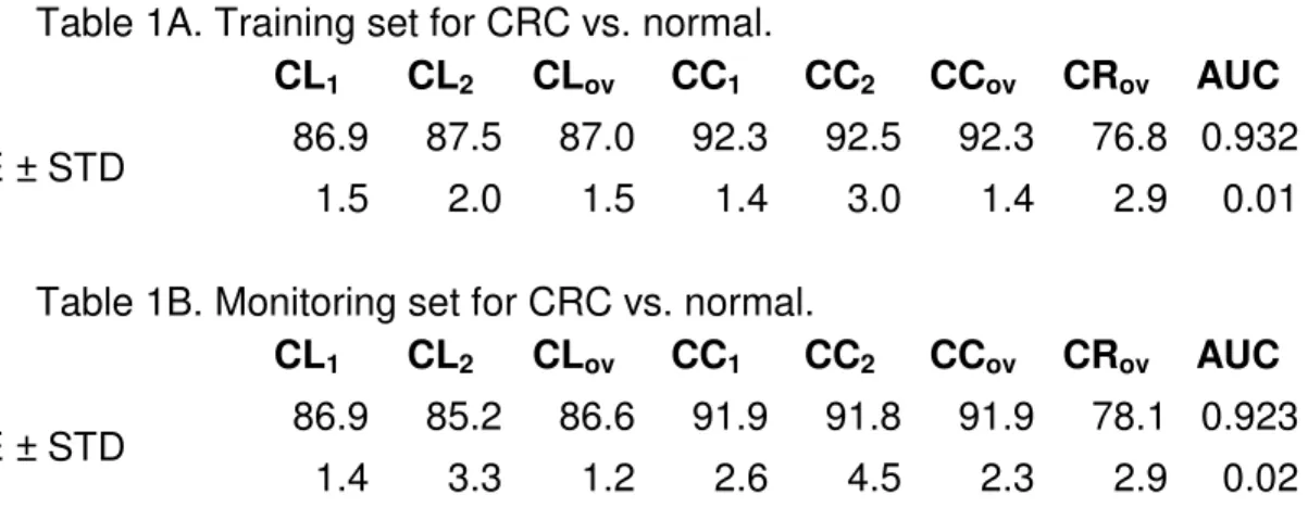
Then ν may be further fine-tuned until we obtain the closest achievable balance. Note that the above approach is not confined to the 2-dimensional CP projections; we used it in e.g., [4] to obtain the FLD-based classification results for the 15-dimensional, non-projected CRC dataset ( Table 1A and Table 1B).

Table 1A. Training set for CRC vs. normal.

CL1 CL2 CLov CC1 CC2 CCov CRov AUC

AVE ± STD 86.9 87.5 87.0 92.3 92.5 92.3 76.8 0.932

1.5 2.0 1.5 1.4 3.0 1.4 2.9 0.01

Table 1B. Monitoring set for CRC vs. normal.

CL1 CL2 CLov CC1 CC2 CCov CRov AUC

AVE ± STD 86.9 85.2 86.6 91.9 91.8 91.9 78.1 0.923

1.4 3.3 1.2 2.6 4.5 2.3 2.9 0.02

For display, it is generally beneficial to transform the raw class proximity dissimilarity matrix D = {δij} into a new matrix Ω = {ωij}, with elements ωij = ln(δij), with ln(·) the

natural logarithm. This logarithmic transformation spreads out the instances in the CP-Plane display, and has theoretical justification for Gaussian distributions [20], [19, pp. 353–356]. Although the distribution of the instances’ location depends on the selected class proximity/distance pair [π; Δ], the subsequent classification of such generalized distributions tends to be more accurate; this will be exemplified later.

We created, and coded in MATLAB, a visualization software we call CPP (Class

Proximity Projector), with which we may display not only the projections for different [π;

Δ] combinations, but also their various iterated versions. In addition, we incorporated

the capability to apply, at any stage, a wide variety of preprocessing steps, including feature selection and different data transformations (both independent and class-specific). When sample size is adequate, multiple random splitting of the dataset into training, monitoring and test sets is also available in CPP, as is the pair-wise

interchanges of the above three sets. Furthermore, we can also import such split datasets for display and additional analysis. An important and visually obvious

advantage is that in the CP plane we may optimize directly the best line separating the two classes [41], either automatically or manually. This involves translating and/or rotating the discriminating line away from the 45° line passing through the origin. We do this by using as the numerical optimization scheme a simple grid search to obtain the two optimal parameters. Note that in CPP we provide two options: minimizing either the classification error or the more general transvariation probability (TVP) [41]; (see also the Conclusion section for a more detailed discussion of TVP).

In Fig. 1, Fig. 2 and Fig. 3 we display different [π; Δ] projections for Fisher’s well known 4-dimensional Iris dataset. We confine ourselves to the two classes that are not

perfectly separable: Versicolor, red disks, 50 instances, Virginica, blue disks, 50

instances. We also show the visual difference between the d1 vs. d2 and ln(d1) vs. ln(d2) projections. Dashed lines represent the optimal class separators (not necessarily the 45° lines that pass through the origins). Disks outside the dotted lines have class assignment probabilities, p 0.75. (The dotted lines representing the boundaries separating p 0.75 from p 0.75 are parallel for the ln(d1) vs. ln(d2) plots [19]).

Fig. 1. Class proximity measure: 3-NN, distance measure: Anderson–Bahadur, with α = 0.22 (optimized for balancing sensitivity and specificity). Here, and in all following Figures, the dashed lines show the best class separators, the dotted ones the 75% probability limits. Points outside these are crisp (p > 75%). Red disks are Versicolor instances (98% accuracy, 34% crisp), blue ones are Virginica ones (98% accuracy, 12% crisp). (For interpretation of the references to color in this figure legend, the reader is referred to the web version of this article.)

Fig. 2. Class proximity measure: Centroid, distance measure: Anderson–Bahadur, with α = 0.39 (optimized for balancing sensitivity and specificity). Versicolor instances (98% accuracy, 36% crisp), Virginica instances (98% accuracy, 20% crisp).

Fig. 3. Class proximity measure: 5-NN, distance measure: symmetric Kullback–Leibler. Versicolor instances (98% accuracy, 0% crisp), Virginica instances (98% accuracy, 0% crisp).

We tuned parameters to achieve the highest accuracies (or lowest transvariation probabilities); note, that the crispness of an instance’s assignment to a specific class depends strongly on the particular [π; Δ] pair chosen.

2. Specific examples, results and discussion

We demonstrate in detail some of the above-described CP-PROJ-based classification options/capabilities on a specific, high-dimensional biomedical dataset, derived from 1H magnetic resonance spectra of non-diseased subjects (controls) and colorectal cancer (CRC) cases [4]. We also apply the methodology to four datasets from the UCI data Repository (http://archive.ics.uci.edu/ml) [14].

2.1. CP-PROJ-based classification of non-diseased vs. CRC dataset

This two-class dataset consists of 412 controls and 111 CRC cases. 1H MR spectra of fecal extracts from the subjects provided the experimental data for which the classifiers were developed.

We required a series of steps (detailed in [4]), based on our Statistical Classification Strategy [40] to produce the results we have reported. In short, these are the steps: (1) We converted the original, 16,384-dimensional complex spectra to magnitude

spectra, and we arrived at 1000 spectral intensities by eliminating spectral regions that appeared to be background noise.

(2) We normalized each spectrum to unit area, aligned all peaks in the dataset, and computed first derivatives that were further rank ordered.

(3) Using the GA-driven feature selector [28], we generated from the processed 1000-intensity spectra 26 features (26 averaged subregions of varying widths),

with FLD/LOO (Fisher’s linear discriminant with leave-one-out crossvalidation) as the wrapper-type classifier. To further improve classification accuracies, we augmented these 26 features with their quadratic terms, resulting in 377 linear + quadratic features.

(4) Ten random 50:50 splits into training (206:55) and monitoring (206:56) produced ten datasets. Applying independently to each of these an approximation to exhaustive feature subset selection (random sampling, repeated many times), with cross-validation we found sets of 15 of the 377 features to be optimal. The reported classification results, shown in the Table 1A and Table 1B were

produced with these 15-feature datasets.

In these tables, CL1, CL2, CLov denote the 15-feature-based classification accuracies for class 1 (Control, CL1≡ Specificity), class 2 (Cancer, CL2≡ Sensitivity), and for the entire data (CLov≡ overall accuracy), respectively. CCk, k = 1, 2 and CCov are the

corresponding “crisp” accuracy results (i.e., when class assignment confidence is 75%); CRov indicates the overall percentage of instances that were found crisp. In the last column, we show the Area Under the Curve (AUC) values of the ROCs. We

computed the average (AVE) and standard deviation (STD) from the individual results obtained for the ten splits.

We balanced training set sensitivities (SE) and specificities (SP) by using

class-dependent instance misclassification penalties as discussed above; we imposed these same penalties on instances in the monitoring sets. For each of the 10 random splits, we balanced the (SE/SP) pairs independently.

Treating the above results as benchmarks, we demonstrate the capabilities and

flexibilities inherent in the Class Proximity Projection approach. Thus, we also start with the same, 1000-point, area-normalized, peak-aligned spectra, however, without the above sketched, specific feature selection steps, addition of quadratic terms, etc. Furthermore, in the following, we didn’t partition the original dataset into training and monitoring sets, as was done for the study published in [4]. This was intentional,

because for this presentation we simply wanted to introduce the CP projection concept and its possibilities, without introducing unnecessary complications and bias due to partitioning the full dataset.

Our starting point of the CP analysis was much simpler, more transparent and more readily interpretable. Our only concession, (to help avoid singular covariance matrices when using FLD), was to partition the 1000-dimensional spectral feature space into ten 100-dimensional subspaces: these adjacent, consecutive, non-overlapping data point ranges were 1–100, 101–200, … , 901–1000. Here and in all subsequent computations, FLD/LOO was the classifier and crossvalidation of choice.

In Table 2, we display the average (AVE) and standard deviation (STD) values,

computed from the individual, direct classification results for the above ten different 100-feature regions. In addition to the above defined CL1, CL2, CLov, CC1, CC2, CCov, CRov,

we also show CR1 and CR2, the class-specific percentages of crisp instances. There is only marginal improvement over a random coin toss (50%), and the STDs are large.

Table 2. Direct application of FLD to the ten 100-feature spectral regions.

CL1 CL2 CLov CC1 CR1 CC2 CR2 CCov CRov

AVE ± STD 55.1 55.0 55.1 56.1 55.4 56.2 53.2 56.1 54.9

4.9 5.0 5.0 6.7 6.2 7.8 6.7 6.7 5.6

There are a large number of possible CP-based mappings from 100 to 2 dimensions. In Table 3 we present the averaged FLD classification results (CP_AVE) obtained for the ten 2-dimensional mappings for the ten subregions, based on the [π; Δ] = [CENtroid; MAHalanobis] projection. (The outcomes for other [π; Δ]s, not reported here, were marginally less accurate, but these differences were not significant statistically.)

Table 3. FLD/LOO results for the ten 100-feature spectral regions after CP projection.

CL1 CL2 CLov CC1 CR1 CC2 CR2 CCov CRov

CP_AVE ± CP_STD 78.9 78.9 78.9 87.6 64.5 91.3 51.5 88.3 61.7

2.8 2.8 2.8 2.5 5.3 2.4 11.1 2.0 6.2

CP_AVE – AVE 23.8 23.9 23.8 32.2 8.3 35.1 −1.7 32.1 6.8

Comparison of the results presented in Table 2 and Table 3 shows statistically

significant improvements for the ten datasets. The last line of Table 3, CP_AVE – AVE, indicates an approximately 23.8% average improvement for the classification

accuracies and an average lowering of the STDs by 2.2%. The requirement that only results above a given confidence level be considered (in this case, that only class assignment probabilities 75% be acceptable), generally increases the classification accuracies, at the expense of having only a fraction of the instances satisfy the 75% threshold. The average improvement in the CCov results is 32.1%; the average

crispness, CRov also improved by 6.8%.

Of the ten spectral subregions, subregion 501–600 gave the worst overall classification results (effectively a random coin toss) when using all 100 attributes of this subregion (see Table 2 for AVE). In Table 4, we present the direct, non-projected FLD/LOO results from this 100 dimensional feature space.

Table 4. Direct FLD/LOO results for spectral subregion 501–600.

CL1 CL2 CLov CC1 CR1 CC2 CR2 CCov CRov

48.3 48.6 48.4 44.9 47.6 50.0 48.6 46.0 47.8

In Table 5 we show the outcomes of five CP mappings from the 100-dimensional subregion 501–600 to 2-dimensional proximity planes, using [CEN; AB(α)] for five equally spaced α values, 0.00(0.25)1.00. AB(α) is the Anderson–Bahadur(α) distance

measure (see the “Distance Measures Δ” section above) and CEN (centroid) is the class proximity measure. Recall that for AB(0.0), only the covariance matrix S1, for AB(1.0), only S2 is used; AB(0.5) ≡ MAH is the Mahalanobis distance.

Table 5. Accuracies for projections from 100 dimensions to CP planes for five AB(α)s. α CL1 CL2 CLov CC1 CR1 CC2 CR2 CCov CRov 0.00 68.7 68.5 68.6 81.4 27.4 81.6 34.2 81.5 28.9 0.25 71.6 72.1 71.7 81.5 44.7 87.5 43.2 82.8 44.4 0.50 75.7 75.7 75.7 85.6 59.0 93.9 44.1 87.0 55.8 0.75 82.0 82.0 82.0 91.5 68.2 95.7 41.4 92.0 62.5 1.00 96.4 96.4 96.4 100.0 79.9 100.0 1.8 100.0 63.3 CP_AVE(α) 78.9 78.9 78.9 88.0 55.8 91.7 32.9 88.7 51.0

Clearly, these results depend very strongly on α. In particular, except for CR2 (the class assignment crispness for the cancer class), all classification accuracy descriptors increase with increasing α; in fact, for the most accurate classification only S2 seems relevant or necessary. CR2 varies non-monotonically with α, ranging from 1.8% to 44.1%, with a median value of 41.4%.

Could we do better? Using the ideas discussed above for generating new feature sets from CP-PROJ-created feature pairs, we combined the five α-based feature pairs (their individual classification results are in Table 5) to create a single 10-feature dataset. In Table 6 we display the classification results obtained for this dataset (no additional projection).

Table 6. Comparison of classification accuracies for various CP-PROJs.

CL1 CL2 CLov CC1 CR1 CC2 CR2 CCov CRov

10-Feature dataset 97.3 97.3 97.3 99.2 92.7 100.0 94.6 99.4 93.1

CP_AVE(α) (Table 5) 78.9 78.9 78.9 88.0 55.8 91.7 32.9 88.7 51.0 10-Feature – CP_AVE(α) 18.4 18.4 18.4 10.8 36.9 8.3 61.7 10.7 42.1 The improvement of the classification outcome for the 10-feature dataset relative to the average of the classification results for the five different αs used (shown in row 2 of Table 6) is statistically significant, especially for the crispnesses.

Consider a new, 10-feature dataset, obtained by combining the five 2-feature [CEN, AB(α)]s. (Their individual classification results are in Table 5.) In Table 7 we collect the outcomes of further projecting this 10-feature dataset to different CP planes by using different [π; Δ]s. In the first row of Table 7 we reproduce, as the baseline, the

classification results presented in the 1st row of Table 6. We only display the best [π; Δ] pairs (listed arbitrarily in decreasing CRov order.) For many other pairs, the results (not shown) were only marginally less accurate.) The abbreviations for the class proximity

measures are: CEN ≡ Centroid, BP ≡ Best Pair (of reference instances, identical to the

RDP mapping), BPT ≡ Best Pair, but the classifier result was obtained by using

Transvariation Probability, AVD ≡ Average Distance, and K-NN ≡ Kth nearest neighbor. For the distance measures, AB(α) ≡ Anderson–Bahadur(α), SKL ≡ Symmetric Kullback– Leibler, MNK(α) ≡ Minkowski(α). Special cases (shown in the Figures) are

MAHalanobis ≡ MAH = AB(0.5) and EUClidean ≡ EUC = MNK(2.0). The last row shows

the average improvement of the ten different 2-dimensional projections relative to the 10-dimensional, pre-projection dataset.

Table 7. Comparison of the baseline with classification results for ten different [π;

Δ]s.

CP-PROJ [π; Δ] CL1 CL2 CLov CC1 CR1 CC2 CR2 CCov CRov

10-Feature set (baseline) 97.3 97.3 97.3 99.2 92.7 100.0 94.6 99.4 93.1

[BPT; AB(0.0)] 100.0 100.0 100.0 100.0 100.0 100.0 100.0 100.0 100.0 [BPT; MNK(0.5)] 99.8 100.0 99.8 99.8 100.0 100.0 100.0 99.8 100.0 [AVD; AB(0.0)] 99.5 100.0 99.6 99.8 99.3 100.0 100.0 99.8 99.4 [17-NN; AB(0.0)] 99.0 100.0 99.2 99.5 99.0 100.0 100.0 99.6 99.2 [BPT; SKL] 99.8 100.0 99.8 99.8 99.8 100.0 96.4 99.8 99.0 [CEN; AB(0.0)] 99.0 100.0 99.2 99.8 98.3 100.0 100.0 99.8 98.7 [CEN; SKL] 98.5 100.0 98.9 99.7 96.4 100.0 100.0 99.8 97.1 [13-NN; EUC] 98.8 100.0 99.0 99.5 97.8 100.0 93.7 99.6 96.9 [AVD; SKL] 98.5 100.0 98.9 99.5 96.1 100.0 99.1 99.6 96.7 [AVD; EUC] 98.1 100.0 98.5 99.7 96.6 100.0 96.4 99.8 96.6 CP_AVE 99.1 100.0 99.3 99.7 98.5 100.0 98.6 99.8 98.4 CP_AVE – baseline 1.8 2.7 2.0 0.5 5.8 0.0 4.0 0.4 5.3

The outcomes in Table 7 demonstrate that when the baseline results are already sufficiently accurate (“sufficiently” is user- and data-dependent), it is essentially irrelevant which of the CP mapping [π; Δ] is used: of the 90 (10 × 9) different class accuracy measures CL1, CL2, CLov, CC1, etc. displayed in the table, only one, shown in

bold (CR2 for [13-NN; EUC]) was somewhat less accurate than the nine class accuracy measures (CL1, … , CRov) shown for the non-projected 10-dimensional dataset. For this dataset, [BPT; Δ] tended to be amongst the best, with [BPT; AB(0.0)] producing a perfect score. Generally, Δ = AB(0.0), i.e., S(0.0) = S2 dominated, suggesting that for this particular dataset, only the covariance matrix (“shape”) of the cancer class was important and necessary for good classification.

When the [π; Δ] projections are parameter dependent, we display only those that give the best results. However, even for these, we did not fully optimize the tunable

parameters for the classifiers. For example, AB(α)s were computed, arbitrarily, only for

α = 0.0, 0.5 and 1.0, MNK(α)s for α = 0.5(0.5)3.0.

Even when the accuracies produced by the various [π; Δ] projections are essentially the same, the actual 2-dimensional displays of these projections may look drastically

different, as Fig. 4 and Fig. 5 vividly demonstrate.

Fig. 4. Class Proximity Projections from the 10-dimensional dataset to two dimensions: [CEN; MAH] (left panel) and [CEN; EUC] (right panel). The blue disks represent the colon cancer instances, the red disks the instances of the healthy class. Note that the [CEN; EUC] projection is considerably crisper than the [CEN; MAH] one. (For interpretation of the references to color in this figure legend, the reader is referred to the web version of this article.)

Fig. 5. Two Class Proximity Projections from the 10-dimensional dataset to two dimensions: [CEN; AB(0.0)] (left panel) and [17-NN; AB(0.0)] (right panel). Note that the [17-NN; AB(0.0)] projection is crisper than the [CEN; AB(0.0)] one.

The CP projections displayed in Fig. 4 and Fig. 5 all have the same classification

accuracies, 98.3% for healthy, 98.2% for colon cancer. The major differences are in the crispness, i.e., the instances appearing outside the dotted lines in the plots. (Compare Fig. 4, [CEN; MAH], no crisp instances, with Fig. 5, [17-NN; AB(0.0)], high fraction of instances crisp.) Notice that the crispness values in the Figures are lower than the corresponding ones shown in Table 7, obtained by FLD/LOO. This is the consequence of the different definition of the (pseudo-)probabilities pk, k = 1, 2 for the Figures. For the

class proximities, pk = dk/(d1 + d2), k = 1, 2, p1 + p2 = 1, and an instance is declared crisp if either of its pk is 0.75. These “probabilities” are distribution independent. For FLD

(and assuming the normal distribution N(0, 1)), = (1/√2π)) .

Furthermore, the tuned FLD/LOO classification does not correspond directly to the displays; the percent crispness values shown in the projection figures are with respect to the 45° line and not with respect to the optimal class separators.

2.2. Iterated [π; Δ] mappings

We may apply more than one consecutive CP mapping to any dataset. In Table 8, we show outcomes of various additional (iterated) mappings, starting from one of the less accurate 2-dimensional projected datasets, [π; Δ] = [CEN; EUC] ≡ I1 (the baseline, first row). Although not the best achievable via CP-PROJ, all accuracy values for I1 are very good, except the crispness value CR2 (and consequently CRov). This is because to obtain the results for I1, we focused on optimally balancing CL1 and CL2, regardless of

the other descriptor outcomes. This happened to give rise to the particularly low CR2 value of 58.6%, shown in underlined bold. For the once-iterated mapping results starting from I1 in Table 8, we again attempted to obtain the best possible balance between CL1 and CL2; however, this time the CR1 and CR2 values also turned out to be better balanced. There are considerable, statistically meaningful improvements in both the individual and the average CR2 and CRov values; this is particularly apparent from CP_AVE – I1 (in bold).

Table 8. Once-iterated mapping results, starting from the first projection

I1≡ [CEN; EUC]. I1→ [π; Δ] CL1 CL2 CLov CC1 CR1 CC2 CR2 CCov CRov I1 ≡ [CEN; EUC] 98.3 98.2 98.3 99.7 96.4 100.0 58.6 99.8 88.3 I1→ [BPT; MAH] 98.5 98.2 98.5 98.5 99.8 100.0 98.2 98.8 99.4 I1 → [BPT; AB(1.0)] 98.5 98.2 98.5 98.5 99.8 100.0 98.2 98.8 99.4 I1→ [BPT; EUC] 98.3 98.2 98.3 98.5 99.8 100.0 98.2 98.8 99.4 I1→ [BPT; MNK(0.5)] 98.1 98.2 98.1 98.5 99.5 98.2 99.1 98.5 99.4 I1 → [BPT; MNK(1.0)] 99.5 97.3 99.0 99.8 99.5 98.2 98.2 99.4 99.2

CP_AVE (five CP-PROJs) 98.6 98.0 98.5 98.8 99.7 99.3 98.5 98.9 99.4

I1→ [π; Δ] CL1 CL2 CLov CC1 CR1 CC2 CR2 CCov CRov

CP_AVE–I1 0.3 −0.2 0.2 1.1 3.3 −0.7 39.9 −0.9 11.1 The result for the once-iterated first mapping I1 = [CEN; EUC], with [BPT; MAH] as the next iterating [π; Δ] pair, i.e., {[BPT; MAH] [CEN; EUC]} is shown in Fig. 6.

Fig. 6. In the right hand panel we show, starting with [CEN; EUC], the result of the subsequent projection using [BP; MAH] (i.e., “once-iterated”, {[BP; MAH][CEN; EUC]} = [BP; MAH] → [CEN; EUC]).

How much further improvement is possible by additional mappings? In Table 9 we display another set of iteration results, starting from the once-iterated I2 ≡ [[CEN; EUC] → [BPT; MAH]], shown in the right hand panel of Fig. 6. We computed CP_AVE and ±CP_STD from the best eight mappings (individual results not shown) that have overall crispness values CRov 99.4% (these are the eight I2s, [CEN; EUC] → [πk;

Δk_{] ≡ [π}k_{; Δ}k_{][CEN; EUC], k = 1, … , 8 prior to any mapping). The eight CP mappings}

[πk; Δk] we used were: [15-NN; MAH], [17-NN; MAH], [CEN; MAH], [BPT; MAH] giving 99.8%, [BPT; AB(1.0)] yielding 99.6% and [BPT; MNK(0.5)], [BPT; EUC], [BPT; SKL] giving 99.4%.

Table 9. Twice-iterated average mapping results, from I2≡ {[BP; MAH] [CEN; EUC]}.

I2 CL1 CL2 CLov CC1 CR1 CC2 CR2 CCov CRov

I2≡ {[BPT; MAH][CEN; EUC]} 98.5 98.2 98.5 98.5 99.8 100.0 98.2 98.8 99.4

CP_AVE (five CP-PROJs) 98.5 98.2 98.5 98.6 99.8 99.1 99.1 98.7 99.6

±CP_STD 0.1 0.0 0.0 0.2 0.2 0.8 0.8 0.1 0.2

CP_AVE – I2 0.0 0.0 0.0 0.1 0.0 −0.9 0.9 −0.1 0.2

On average, CR2 still improves slightly (0.9%), but with a concomitant small decrease (0.9%) for CC2. This suggests that additional mappings will be neither necessary nor beneficial. This is borne out in Fig. 7, where we show a twice-iterated mapping

Fig. 7. Twice-iterated projection, starting with the once-iterated I2≡ {[BP; MAH] [CEN; EUC]}, with [CEN;

SKL] as the second iteration, i.e., {[CEN; SKL] [BP; MAH] [CEN; EUC]}. Notice that the second iterated projected dataset has no crisp instances.

2.3. CP-PROJ-based classification of four datasets from the UCI repository

Are the good results shown for the originally 1000-dimensional biomedical dataset accidental? To test this, we selected four, frequently used 2-class datasets from the UCI data Repository (http://archive.ics.uci.edu/ml): Pima Indians Diabetes, BUPA (Liver Disorder), Sonar and Ionosphere. All pertinent information is collected in Table 14, which includes our best classification results, an earlier study using SVM with a Gaussian kernel [43] and the best results obtained with a sophisticated classifier approach that used a scatter-search-based ensemble, with SVM as one of the three base classifiers [8]. Note that after the appropriate CP-PROJ, we classified the four UCI datasets using the concept of transvariation probability (TVP) [26], [7] and [41].

Table 14. % Accuracies of 10-fold CV test sets of UCI datasets, CP-PROJs and two SVMs. No. Samples Features CP-PROJ ± STD SS-SVM (%)b LS-SVM (%)a Pima diabetes 268 + 500 8 76.5 ± 4.4 82.8 77.3 BUPA liver 145 + 200 6 80.9 ± 8.8 81.4 69.4 Ionosphere 225 + 126 34 98.2 ± 2.4 99.3 95.6 Sonar 97 + 111 60 100.0 ± 0.0 98.2 77.9

a T. Van Gestel, J.A.K. Suykens, G. Lanckriet, A. Lambrechts, B. De Moor, J. Vandewalle A bayesian framework for least squares support vector machine classifiers, gaussian processes and kernel fisher discriminant analysis Neural Comput, 14 (5) (2002), pp. 1115–1147

b Sh-Ch. Chen, S.h.-W. Lin, Sh-Y Chou Enhancing the classification accuracy by scatter-search ensemble approach Appl Soft Comput, 11 (2011), pp. 1021–1028 Classification by TVP has many advantages not shared by other linear classifiers. It is more general than FLD: for classification we may use any 1D projection i.e., a line not

confined to be the one traversing the two class means. (This is the fundamental concept behind projection pursuit[16]. The best projection is determined by optimizing some pre-selected objective function, or by generating a large number of random projections and identifying the optimal one by some classification-based measure.) Furthermore, unlike with the FLD, the classification results obtained are more robust against outliers on the discriminating projection line. This is because (again unlike the FLD), the TVP classifier is nonparametric: it only involves counts (the minimum number of “jumps” required to optimally separate the two classes on the projection line); hence it does not depend on homocedasticity and normality assumptions for optimality. In addition, a TVP classifier provides more information than a minimum error classifier that only delivers the number of misclassifications. Thus, for a given misclassification error, there may be different TVP results, depending on the “depth” by which the misclassified instances are

immersed in the “wrong” class [41]. This confirms that the procedure leading to TVP is more general than classification; it is based on ranking.

In Table 10, Table 11, Table 12 and Table 13, we show our classification outputs for the four UCI datasets. For each dataset, its Table contains the result for the best, final CP mapping, its LOO CV result, as well as the 5-fold and 10-fold crossvalidation outcome for the test set. For the 5-fold and 10-fold CVs we also show the standard deviations (STDs). Note that depending on the dataset, the end product of the best CP mapping may be different: it may have been arrived at by singly-, or multiply-iterated mappings, or even by more complicated combinations of mappings.

Table 10. Pima diabetes. Various CV results (test set): 268 Class 1, 500 Class 2 instances. CL1 CL2 CLov CC1 CR1 CC2 CR2 CCov CRov CP-PROJa 78.0 78.0 78.0 88.8 56.7 87.5 59.4 88.0 58.5 LOO 75.4 76.4 76.0 87.7 57.5 87.2 59.2 87.3 58.6 5-Fold CV ± STD 77.2 77.2 77.2 88.9 56.7 87.7 59.6 88.2 58.6 5.1 5.4 2.9 6.0 4.2 5.8 6.4 3.4 3.9 10-Fold CV ± STD 76.1 76.8 76.5 88.2 57.9 87.6 59.0 87.8 58.6 6.7 6.9 4.4 8.0 7.0 6.9 7.5 4.3 4.8

a Using the final classifier generated from the last completed stage.

Table 11. Sonar. Various CV results (test set): 97 Class 1, 111 Class 2 instances.

CL1 CL2 CLov CC1 CR1 CC2 CR2 CCov CRov

CP-PROJa 100.0 100.0 100.0 100.0 100.0 100.0 100.0 100.0 98.6

CL1 CL2 CLov CC1 CR1 CC2 CR2 CCov CRov 5-Fold CV ± STD 100.0 100.0 100.0 100.0 96.9 100.0 100.0 100.0 98.6

0.0 0.0 0.0 0.0 2.5 0.0 0.0 0.0 1.2

10-Fold CV ± STD 100.0 100.0 100.0 100.0 97.1 100.0 99.1 100.0 98.1

0.0 0.0 0.0 0.0 4.5 0.0 2.7 0.0 2.4

a Using the final classifier generated from the last completed stage.

Table 12. Ionosphere. Various CV results (test set): 225 Class 1, 126 Class 2 instances.

a Using the final classifier generated from the last completed Stage.

Table 13. BUPA liver. Various CV results (test set): 145 Class 1, 200 Class 2 instances. CL1 CL2 CLov CC1 CR1 CC2 CR2 CCov CRov CP-PROJa 81.4 81.5 81.4 92.2 71.0 84.4 48.0 88.4 57.7 LOO 81.4 81.5 81.4 91.3 71.7 84.4 48.0 88.0 58.0 5-Fold CV ± STD 81.0 80.5 80.6 91.2 71.9 85.7 49.0 8.4 58.6 5.9 8.6 6.7 5.1 4.6 9.4 5.9 6.3 5.1 10-fold CV ± STD 81.3 80.9 80.9 91.1 72.0 84.9 47.9 88.3 57.8 7.7 11.2 8.8 6.9 7.1 12.1 12.0 8.5 10.2

a Using the final classifier generated from the last completed stage.

Below, we show the details of the CP-PROJ combinations we used for the four datasets. They are ordered in increasing processing complexity. The notation [π;

Δ][Stage k] indicates additional mapping using some particular [π; Δ], applied to the

outcome of previous mappings and feature combinations used at [Stage k]. Interestingly, for the Pima Indians data, we could not improve significantly the classification results beyond what we found (see Table 14), even when trying to increase the numbers and types of [π; Δ]. In contrast, it is easy to obtain excellent

CL1 CL2 CLov CC1 CR1 CC2 CR2 CCov CRov CP-PROJa 98.2 98.4 98.3 98.7 99.6 99.2 99.2 98.9 99.4 LOO 98.2 98.4 98.3 98.2 100.0 98.4 100.0 98.3 100.0 5-Fold CV ± STD 98.7 98.4 98.6 98.7 99.6 98.4 100.0 98.6 99.7 1.1 2.0 0.9 1.1 0.9 2.0 0.0 0.9 0.6 10-Fold CV ± STD 98.2 98.3 98.2 98.6 99.6 98.3 100.0 98.5 99.7 3.0 3.3 2.4 2.9 1.4 3.3 0.0 2.4 0.9

results for the Sonar dataset: with the TVP-based linear classifier, even direct classification from the original 60 dimensional feature space gave 80.8% accuracy, while imposing optimally balanced sensitivity and specificity. Furthermore, any one of the three CP-PROJs on its own, comprising Stage 1, already achieved 96.2% accuracy. It is noteworthy that for all four datasets their three CV results are quite similar. As expected, the STDs are larger for the 10-fold CVs.

2.3.1. Pima Indians diabetes

Stage 1: {[CEN; AB(1.0)] + [CEN; SKL]} (4 features);

Stage 2: Best 3 features: 1, 2, 4; exhaustive search from Stage 1 result 2.3.2. Sonar

Stage 1: {[CEN; AB(0.00)] + [3-NN; SKL] + [1-NN; SKL]} (6-feature dataset, created from 3 independent projections).

Stage 2: Best 4 features: 1, 2, 3, 5; exhaustive search from the six Stage 1 features

2.3.3. Ionosphere

Stage 1: {[CEN; SKL] + [AVD; SKL] + [AVD; MAH] + [BPT; MAH]} (8-feature dataset, created from 4 independent projections).

Stage 2: [BPT; SKL][Stage 1] (2 features) 2.3.4. BUPA (liver disease)

Stage 1: {[CEN; AB(0.00] + [CEN; MAH] + [CEN; AB(1.00] + [AVD;

MAH] + [AVD; AB(1.00)] + [BPT; MAH]} (12-feature dataset, created from the above 6 independent projections).

Stage 2: {[CEN; MAH][Stage 1] + [AVD; AB(1.00)][Stage 1] + [9-NN; SKL][Stage 1]+

[BPT; SKL][Stage 1] + [5-NN; MAH][Stage 1]} (10-feature dataset, created from the above 5 independent mappings).

Stage 3: {[CEN; SKL][Stage 2] + [11-NN; SKL][Stage 2] + [BPT; SKL][Stage 2] + [7-NN; AB(0.00)][Stage 2]} (8-feature dataset, created from the above 4 independent mappings).

Stage 4: {[11-NN; MAH][Stage 3] + [9-NN; MAH] [Stage 3] + [7-NN; MAH][Stage 3] + [CEN; MAH][Stage 3]} (8-feature dataset, created from the above 4

independent mappings).

In Table 14 we compile pertinent information on the four UCI datasets and compare our 10-fold CV accuracies with the corresponding LS-SVM ones based on Radial Basis

Function kernels [43] and with results obtained via SS-SVM, a sophisticated ensemble approach [8], using scatter search optimization [25]. From Chen’s 9-classifier ensemble results, we quote only the best of three SVM outcomes for the test data.

Inspection of the table reveals that CP-PROJ outperformed LS-SVM on three of the four

datasets (LS-SVM’s accuracy for Pima Diabetes was in the CP-PROJ range). SS-SVM

did better on the Pima Diabetes dataset, and somewhat worse on the Sonar data. No statistically significant differences were found between the CP-PROJ and SS-SVM results for the BUPA and Ionosphere data.

As an additional test of the CP projection approach, in Tables 15A (full dataset), 15B (training set) and 15C (monitoring set) we display the classification results for the split Ionosphere data. The particular training/monitoring split we used is the one presented in the Repository.

Table 15A. Ionosphere. Average results, all instances: 225 Class 1, 126 Class 2 instances.

CL1 CL2 CLov CC1 CR1 CC2 CR2 CCov CRov Direct, with 34 features 82.2 82.5 82.3 91.4 77.8 88.2 87.3 90.2 81.2

Best: [7-NN; MAH] 95.6 96.0 95.7 97.0 88.9 97.5 93.7 97.2 90.6

CP_AVE 93.6 93.9 93.7 96.9 86.5 96.0 92.3 96.6 88.5

±CP_STD 1.9 1.8 1.8 2.2 6.4 2.4 5.9 2.1 6.1

CP_AVE – direct 11.4 11.4 11.4 5.5 8.7 7.8 0.9 6.4 7.3

Table 15B. Ionosphere. Average results, training set: 101 Class 1, 99 Class 2 instances.

CL1 CL2 CLov CC1 CR1 CC2 CR2 CCov CRov Direct, with 34 features 82.1 81.8 82.0 78.3 59.4 88.6 79.8 84.2 69.5

Best: [3-NN; MAH] 93.1 93.9 93.5 98.9 88.1 94.5 91.9 96.7 90.0

CP_AVE 92.0 92.6 92.3 97.2 80.3 95.5 86.4 96.4 83.3

±CP_STD 1.9 2.1 2.0 2.5 9.9 2.2 7.3 2.1 8.0

CP_AVE – direct 9.9 10.8 10.3 18.9 20.9 6.9 86.4 12.2 13.8

Table 15C. Ionosphere. Average results, monitoring set: 124 Class 1, 27 Class 2 instances.

CL1 CL2 CLov CC1 CR1 CC2 CR2 CCov CRov Direct, with 34 features 73.4 92.6 76.8 83.0 42.7 90.9 81.5 85.3 49.7

Best: [CEN; MAH] 98.4 92.6 97.4 99.2 97.6 92.3 96.3 98.0 97.4

CP_AVE 95.4 93.4 95.0 98.0 81.5 96.1 91.8 97.7 83.4

±CP_STD 4.7 2.5 3.7 2.9 12.7 2.7 6.3 2.1 11.3

CP_AVE – direct 22.0 1.6 18.2 15.0 38.8 5.2 10.3 12.4 33.7

In the first row of each Table we show the classification results when using all 34 original features; the accuracies range between ∼77% and 82%. We then completed the following 9 CP-PROJs: [CEN; AB(0.00)], [CEN; AB(1.00)], [CEN; MAH], [AVD; MAH], [1-NN; MAH], [3-NN; MAH], [5-NN; MAH], [7-NN; MAH], [BPT; MAH]. In row 2 we show the best of the 9 CP-PROJ accuracies we obtained. Note, that the best [π; Δ]s turned out to be different for the non-split, training and monitoring sets. Rows 3 and 4 contain the average accuracy values CP_AVE and their STDs computed from these 9 projections. The last row shows CP_AVE – Direct, the percent improvement over the direct classification. As might be expected, the results for the monitoring set are much more variable than those for the training set. This is particularly noticeable for the direct classification (e.g., compare CL1 and CL2).

3. General comments and conclusions

We used the entire datasets for the majority of results presented. This is sufficient to demonstrate the various characteristics and possibilities of the 2-dimensional CP projections. Furthermore, this usage is legitimate (consider it as a wrapper-type feature generation, i.e., using class label information to compute the two distances derived from the particular [π; Δ] chosen), since we may simply consider the CP-PROJ as a feature generation procedure prior to the final classifier development. The various

projections/mappings are generators of different 2-dimensional feature sets. The customary splitting into training, validation/monitoring and (when the dataset size

allows) independent test sets would be carried out on the generated 2D dataset. As with any wrapper-based method, results for an independent test set are likely to be less accurate. The extent of the potential overfitting is obviously dataset-dependent; its detailed evaluation over the various datasets was beyond the intended scope of this work. However, our initial assessment, shown in Table 15A, Table 15B and Table 15C for the Ionosphere dataset from the UCI Repository suggests that, at least in this case, no overfitting occurred and training and independent test set accuracies were

statistically equivalent. Furthermore, our 5-fold or 10-fold CV test set results for the four UCI datasets suggest good generalization capability.

Of course, any instance, whether from the training, monitoring or independent test set has to be submitted to the entire projection procedure. Furthermore, if the two classes were preprocessed differently, then we first have to assume that the unknown belongs to class 1, preprocess it accordingly and then assign it; next, we treat it as a class 2 instance, again preprocess it appropriately and then assign it to a class. Based on these outcomes, we shall have to decide to which class we should finally assign the instance. The simplest nonparametric choice could be based on the relative position of the

instance with respect to the 45° line.

The CP-PROJ results typically surpass or at least match the classification accuracy obtainable for the initial high-dimensional dataset. This suggests that how the

preliminary feature set was obtained is less critical than generally thought. For the large, high-dimensional biomedical dataset we studied in detail, once CP-PROJ was applied, the worst spectral region, 501–600 data points, gave only marginally poorer results than the best region, 801–900 (results for the latter not shown).

After combining J different 2-dimensional CP-PROJ-derived feature sets into a single, 2J-dimensional one, and then selecting M-dimensional (M < 2J) feature subsets, the classification accuracies obtained depend on M weakly, if at all. However, with

decreasing M, classification crispness generally decreases. In contrast, subsequent CP iterations generally increase crispness, while preserving the accuracies.

CP-projected datasets have additional flexibility: from the same dataset and original feature set, different 2D feature sets may be generated by using different proximity and distance measures. Using quadratic extensions of any 2D CP-projected dataset leads to 5D feature sets only; these are either directly applicable for classification or available for

another CP-PROJ. (Linear classifiers in the CP-PROJ plane generally correspond to nonlinear ones in the original feature space).

For the majority of the CP projections created, the best class-separating line in the CP plane is not the 45° line that goes through the origin. This is partly so because for the displays we optimized the balance between SE and SP; this balancing generally

required the translation and/or rotation of the initial, 45° class-discriminating line. For the 2D displays, in our CPP software we determine the optimal translation and rotation automatically, by a simple grid search. This was carried out for all calculations on the four UCI datasets.

Why the CP-PROJ? When L < N, the possibility of generating diverse, [π; Δ]-projection-based 2D feature sets is both very attractive and powerful. The ready visualizability of the distribution of the instances in the CP plane, including the immediate identification of possible outliers is a bonus, and so is the possibility of developing effective classifiers. In fact, the two-parameter (position and angle)-based classifier we proposed in [41] is simple to implement, since via the CP-PROJ we have replaced a possibly complicated separating manifold by a line or a nonlinear, 1-dimensional curve.

For L N, direct CP-PROJ is more limited because of the likely singularity of S−1. Unless S is regularized, this confines CP-PROJ to mappings based on the Minkowski measure MNK(α). To access the more powerful and flexible CP-PROJs that depend on computing the covariance matrices, the cardinality M of the modified feature set must satisfy M < N. Such feature set reduction via CPP seems to have the characteristics that the distances based on the two proximity measures generally contain both

discriminative and irrelevant or strongly correlated original features, but there is no need to explicitly separate them. It appears that as long as sufficient discriminatory

information is retained by the CP-PROJ, the resulting 2D classifiers will be at least as accurate as the ones based directly on the M-feature dataset.

In summary, we explored the concept of projecting/mapping high-dimensional datasets to two dimensions, based on pre-determined class proximity – distance measure pairs [π; Δ]. Specifically, we introduced the concept of combining multiple

projections/mappings. First, by selecting, say J different [π; Δ]s and carrying out for

each a CP projection, we generate J separate datasets, each with its own pair of features. With these we may create J different classifiers. We may also construct from these J 2-feature datasets a single 2J-feature dataset for which we may readily develop another classifier. Because 2J is typically O(1), exhaustive search is feasible for

identifying possibly more accurate subsets of the 2J features. We may also use the J classifiers as J “components” for the more conventional classifier aggregation

approaches [23]. By choosing sufficiently different [π; Δ] pairs, we may readily introduce

diversity into the created classifiers (a good example is shown in Table 5); this is one of

the requirements for creating robust classifier ensembles that generalize well [23]. We also introduced the notion of iterated CP mappings. This extends the idea of projecting with an initial, pre-selected [π0; Δ0] pair from the original M-dimensional feature space, M > 2 to a CP plane. Iteration implies that we continue with additional