Biomedical solid state NMR : an ADRF cross polarization study of calcium phosphates and bone mineral

(1)

Biomedical Solid State NMR: An ADRF Cross Polarization Study of

Calcium Phosphates and Bone Mineral

by

Chandrasekhar Ramanathan B. Tech., Electrical Engineering

Indian Institute of Technology, Bombay (1988) M.S., Biomedical Engineering and Mathematics University of North Carolina at Chapel Hill (1990)

SUBMITTED TO THE HARVARD-MIT DIVISION OF HEALTH SCIENCES AND TECHNOLOGY AND THE DEPARTMENT OF NUCLEAR ENGINEERING

IN PARTIAL FULFILLMENT OF THE REQUIREMENTS FOR THE DEGREE OF Doctor of Science

in

Radiological Sciences at the

Massachusetts Institute of Technology May 1996

@ 1996 Chandrasekhar Ramanathan

The author hereby grants to MIT permission to reproduce and to distribute publicly paper and electronic copies of this thesis document in whole or in part.

Signature of Author ...

Harvard-MIT Division of Health Sciences and Technology, and DeDartment of Nuclear Engineering, May 1996 Certified by ...

Professor Jerome L. Ackerman Thesis Supervisor

Approved by ...

C- Professor David Cory Reader Frotessor Sidney Yip Reader Accepted by...

v Professor Jeffrey P. Friedberg ,••.sA;-- ftih iDipartmental Committee on Graduate Students

OF TECHNOLOGY

JUN 2 01996 Science

(2)

Biomedical Solid State NMR: An ADRF Cross Polarization Study of

Calcium Phosphates and Bone Mineral

by

Chandrasekhar Ramanathan

Submitted to the Harvard-MIT Division of Health Sciences and Technology and the Department of Nuclear Engineering on May 14, 1996 in Partial Fulfillment of the

Requirements for the Degree of Doctor of Science in Radiological Sciences

Abstract

This thesis investigates the application of a low power solid state NMR technique, using proton to phosphorus-31 cross polarization via adiabatic demagnetization in the rotating frame (ADRF-CP), to study samples of synthetic calcium phosphate and bone mineral.

The first section describes the use of ADRF-CP, with a surface coil, to detect monohydrogen phosphate ions in the presence of a large background of non-protonated phosphate ions in porcine bone and a mixture of synthetic calcium phosphates. Tran-sient oscillations were observed in the transfer of polarization between the proton dipolar and phosphorus Zeeman nuclear spin reservoirs after the initiation of thermal contact. Suppression of the non-protonated phosphate was achieved by detecting the signal when the oscillation was passing through zero, and adjusting the phosphorus rf field to achieve optimal cross polarization with the proton local fields of the monohy-drogen phosphate ions. An adiabatic remagnetization of the phosphorus eliminated the oscillations, while increasing the strength of the observed total phosphorus signal. The second section describes the investigation of three variants of the ADRF process as well as a Jeener-Broekaert pulse sequence to create proton dipolar order in the calcium phosphates. The relative efficiencies of the different techniques were sample dependent, with the ADRF techniques performing well in hydroxyapatite and poorly in brushite. The reason for this poor performance in brushite is not well understood.

The third section describes experiments demonstrating an ADRF-CP variant of the differential cross polarization technique. The inversion of the phosphorus Zeeman temperature is performed by changing the phase of the phosphorus rf by 180 degrees during the cross polarization. Transient oscillations were observed on inverting the phosphorus temperature.

The final section of the thesis describes the design and construction of a two-port double resonance probe with interchangeable coils for a 4.7 T magnet. The plug-in design for the coils facilitates the use of coils of different circuits and geometries with the same set of variable tuning and matching capacitors. Two double resonance coils were constructed, a surface coil using a novel circuit design, and a previously described cylindrical resonator.

Thesis Supervisor: Jerome L. Ackerman

Associate Professor of Radiology Harvard Medical School

(3)

Acknowledgments

There have been so many people who have taught me so much and enriched my life over the last six years here at MIT that I don't really know where to begin. None of this work would have been possible without the support and guidance of Jerry Ackerman. He has been both a friend and a mentor over the last two years. Working with him has helped me rediscover my fascination with science.

Eric McFarland, Jacqueline Yanch, David Cory and Sidney Yip have provided invaluable advice through the years. Bettina Pfleiderer and Yaotang Wu helped me get my research up and running in the lab. The researchers and staff at the MGH-NMR center have created a friendly and truly stimulating research environment in which I have enjoyed working. The staff in the Nuclear Engineering Department and HST have definitely made my life easier with all their help.

Dick Eckaus and Henry Jacobi gave me a job when I needed it badly, helping me continue my studies. A special thank you to Bruce Rosen whose counselling prevented me from dropping out when things were at their worst. Lauren Johnston,

Paul Whitworth, Jane Song, Lindsay Haugland, Peter Madden, Rene Smith and Helen Turner have taught me the true meaning of friendship. Thank you for the memories. My parents first set me on this path to discovery and gave me the focus to reach my goals. My brother Kumar has stood by me through everything. My debt to him can never be repaid.

(4)

"To follow knowledge like a sinking star, Beyond the utmost bound of human thought."

-- Ulysses, Alfred, Lord Tennyson

Like the sharp edge of a razor, the sages say, is the path. Narrow it is, and difficult to tread.

-Katha Upanishad

"Toutes les transformations sont possibles."

(5)

List of Figures

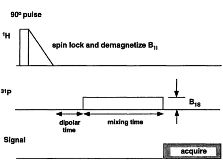
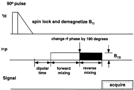
2-1 Spin reservoirs and interations for a system containing a single spin species . . . . 32 2-2 Spin reservoirs and interations for a system containing two spin species 36 2-3 Pulse sequence for the ADRF cross polarization experiment ... 40 2-4 Pulse sequence for the ADRF differential cross polarization experiment. 44 3-1 ADRF-CP signal of BRU as a function of cross polarzation time . . . 49 3-2 ADRF-CP signal of HA as a function of cross polarzation time . . .. 51 3-3 ADRF-CP spectra of a mixture containing 10% BRU and 90% HA as

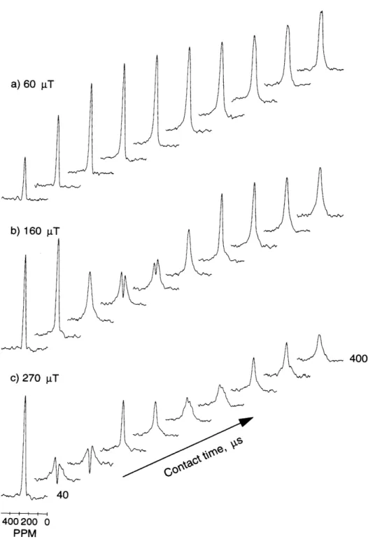
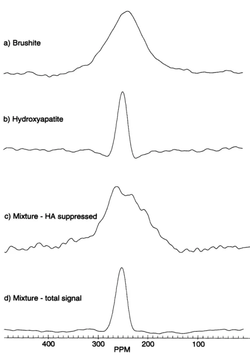
a function of cross polarzation time and B1 field strength ... 53 3-4 ADRF-CP spectra of HA, BRU and a mixture containing 10% BRU

and 90% HA showing PO3- suppression . ... 54 3-5 ADRF-CP spectra of a specimen of porcine bone as a function of

cross-polarization time ... 55 3-6 ADRF-CP spectra of a porcine bone specimen showing PO3- _{suppression 56} 3-7 ADRF-CP signal of HA and BRU after ARRF of the phosphorus . 58 4-1 Detection of proton dipolar order using an ARRF of the phosphorus

spins . . . .. .. . 64 4-2 HA signal after a 7/2 pulse and ramp demagnetization of the spin lock

field ... ... ... 66

4-3 BRU signal after a 7r/2 pulse and ramp demagnetization of the spin lock field . . . .. . 67

(9)

4-5 BRU signal following an adiabatic sweep onto resonance and ramp

demagnetization of the spin-lock field . ... . . . 69

4-6 HA signal following an adiabatic sweep onto resonance with a weak rf field . . . . . . . ... 71

4-7 BRU signal following an adiabatic sweep onto resonance with a weak rf field ... 72

4-8 HA signal following a Jeener-Broekaert sequence . ... 74

4-9 BRU signal following a Jeener-Broekaert sequence . ... 75

5-1 Pulse sequence for ADRF differential cross polarization following ARRF of the phosphorus ... .. ... .. .. .. .. .. 80

5-2 ADRF-DCP experiment on BRU with a step 31P rf . ... 82

5-3 ADRF-DCP experiment on HA with a step 3 1_{P rf . ...} ₈₃

5-4 ADRF-DCP experiment on porcine bone with a step 31P rf ... 86

5-5 ADRF-DCP spectra of a specimen of porcine bone as a function of reverse CP tim e .. .... ... ... ... .. . . .. ... . 87

5-6 ADRF-DCP spectra of a specimen of porcine bone showing linewidth changes . . . .. .. . 88

5-7 ADRF-DCP experiment on BRU following an ARRF of the 31P rf . . 89

5-8 ADRF-DCP experiment on HA following an ARRF of the 31_{P rf}_. _{. .} ₉₀

6-1 A sketch of the constructed probe . ... . 94

6-2 Schematic branch diagram of the double resonance circuit ... 95

6-3 P-SPICE representation of the double resonance circuit ... 98

(10)

List of Tables

3.1 Experimental conditions for ADRF-CP spectra ... . . ... 48

4.1 Experimental conditions for creation of dipolar order ... 63

4.2 Relative degree of dipolar order creation in hydroxyapatite ... 75

4.3 Relative degree of dipolar order creation in brushite ... 76

5.1 Experimental conditions for surface coil ADRF-DCP spectra ... 79

(11)

Chapter 1 Introduction

Bone mineral research has grown in recent years, spurred by public health concerns over osteoporosis [1, 2, 3]. While the mineral is often considered to be the inert, inorganic component of bone whose sole function is to provide mechanical support, it has long been known that there is continual remodeling of bone throughout life, with resorption of older bone mineral and synthesis of new mineral. This process allows the bone to grow, to play its role as a reservoir of calcium and phosphorus, and to maintain its structural integrity by repair of defects and trauma. Many aspects of this remodeling process are poorly understood, and additional knowledge of bone mineral dynamics will be central to our understanding of fracture healing, the determinants of bone strength, and the treatment of metabolic bone diseases such as osteoporosis

[4, 5, 6, 7].

Various physical and chemical techniques have been brought to bear in the study of bone mineral chemistry. These include x-ray diffraction [8, 9, 10, 11], neutron diffraction, back-scattered electron beam imaging [12, 13, 14], wet chemical analyses [15], FT-IR spectroscopy [16, 17, 18, 19, 20] and solid state NMR spectroscopy. The NMR studies are discussed later in this chapter. While each of these techniques has contributed to our current understanding of the chemistry of bone mineral, none of them has been able to provide a detailed, comprehensive description of the process of mineral deposition and resorption. In particular, most of these techniques are destructive, requiring extensive sample preparation that could significantly change

(12)

the local micro-environment of the mineral, as well as its surface chemistry.

An understanding of the chemical dynamics of bone mineral may provide insights into bone growth and metabolic bone disease processes, as well as enable the de-sign of superior antiresorptive pharmaceuticals and bone mineral markers for nuclear medicine scans. Among the established methods, only nuclear medicine techniques, by virtue of the chemical selectivity of a radionuclide-bearing ligand that binds to the surface of bone mineral, have potential for yielding chemical information on the mineral in vivo. However, this information is strictly limited to the surface of bone crystallites, and in practice is used merely to detect regions of high or low remodelling activity [21].

The goal of this work is to exploit the superior ability of NMR spectroscopy to discriminate subtle chemical differences (as between PO'- _{and HPO - ions) in the in}

vivo study of bone mineral. Conventional solid state NMR techniques are generally

incompatible with in vivo application due to the high levels of rf power deposition and the use of magic angle sample spinning. NMR diagnostic techniques, both spec-troscopy and imaging, have thus generally been limited to liquid state studies of soft tissues. It has so far not been possible to use the chemical sensitivity of the NMR methodology to obtain chemical information in vivo from solid tissues such as bone. We require a method which maintains chemical contrast under conditions of low spectral resolution, and minimizes the application of rf power. Cross polarization by means of adiabatic demagnetization in the rotating frame (ADRF-CP) satisfies these requirements. The development of in vivo solid-state NMR techniques would allow the study of bone mineral chemistry in live subjects, and thus overcome the problems due to sample preparation, and the questionable validity of extrapolating the results of studies conducted ex vivo to the in vivo case. The clinical utility of such techniques could possibly extend to monitoring the healing of fractures, the re-sorption and remodelling of bone cements or implants and the treatment of metabolic bone diseases such as osteoporosis and osteomalacia.

(13)

1.1 Introduction to bone tissue

Bone is a composite tissue whose properties closely depend on its structure and com-position. The tissue consists of a network of connective tissue fibers interspersed with bone cells lying in an extracellular ground substance that is impregnated with cal-cium salts to produce rigidity. The orientation of the collagen fibers, which account for about 95% of the organic matter in the tissue, in the extracellular matrix usually determines the spatial arrangement of the mineral crystals deposited in the matrix, and hence the load bearing axes of the the bone. The fibers are randomly arranged in woven bone while showing preferential orientations in lamellar bone. The matrix also contains non-collageneous proteins such as osteonectin and osteocalcin.

1.1.1 Bone cells

The cellular constituents of bone are osteoblasts, osteocytes, lining cells and osteo-clasts [22].

Osteoblasts are responsible for the synthesis and secretion of the organic con-stituents of the bone matrix and, to some extent, their calcification. The osteoblasts are cuboidal or low columnar cells that form a continuous layer on the growing osseous surface, and are usually found with part of their peripheral membrane in contact with the calcification front.

Osteocytes are the least known of the bone cells due to their localization within enclosed lacunae in the calcified matrix. They are formed from osteoblasts that are gradually buried in a calcified matrix, and are thought to undergo three phases. During the formative phase the newly formed ostecyte still shows osteoblastic activity. In the resorptive phase the osteocyte is capable of resorbing the bone matrix which forms the border of its lacuna, while in the degenerative phase the cell fragments and eventually disappears.

The lining cells are a layer of very flat endothelial-like cells that cover the inactive surfaces of bone. They are very thin and their function is practically unknown, though they might play a role in separating the interstitial from the bone fluids.

(14)

Osteoclasts are giant, multinucleated cells attached to the bone surface whose fuction is to resorb bone. The actual mechanism of mineral resorption is not very well understood, though current findings support an extracellular dissolution of the bone mineral followed by digestion of the organic components.

Normal bone metabolism involves continuous bone remodelling which occurs at the level of the bone remodelling unit, also called the "basic multicellular unit" or BMU [23]. Bone volume must be maintained constant during the remodelling by tight coupling between osteoblastic and osteoclastic activity. A BMU goes through different phases of a dynamic process which begins with the activation of osteoclasts on the bone surface (activation phase), continues with the resorption of bone ma-trix and formation of Howships's lacuna (resorption phase), the disappearance of the osteoclasts which are substituted by mononuclear cells (reversion phase), and the disappearance of these cells and reappearance of osteoblasts with reparation of the resorption lacuna (formation lacuna). The local mechanisms which regulate the cou-pling between osteoblastic and osteoclastic activity are not well understood and await further study.

1.1.2 Bone mineral chemistry

The study of the physico-chemical properties of the mineral component of skeletal tissue has advanced significantly since Neuman and Neuman's pioneering treatise on the subject [15]. The dominant apatitic phase has been well characterized, and the dynamics of calcium phosphate precipitation in aqueous solution and in vitro systems reasonably well understood. However, in vivo deposition processes are less well understood and their study poses a significant challenge. The following discussion draws heavily on some recent review articles on the state of bone mineral chemistry research [24, 25].

The first step in the formation of the mineral is the nucleation of the crystal, the creation of a small cluster of ions capable of growth and survival as a crystal. A necessary thermodynamic condition for nuclei formation is that the Gibbs free energy of the reactant ions in solution exceed the free energy of the precipitated

(15)

phase. Otherwise any crystals that formed would quickly dissolve again. In addition, the energy expended in creating the cluster surface should exceed the energy released by ion bonding within the crystal. This energy barrier can be quite high for sparingly soluble salts such as apatites, and must be lowered substantially for nucleation to take place on a reasonable time scale.

The presence of foreign solids can lower the threshold for nucleation to occur if they

1. have a strong affinity for the ions being precipitated, and

2. have a surface topology closely matching that of the precipitated surface. The dimensions of an apatitic nucleus is probably on the order of 1-2 nm [26], which is much smaller than the size of a bone crystal. Crystal growth then accounts for most of the subsequent increase in the mass of the crystal.

There has been much debate on the exact chemical nature of the first calcium phosphates precipitated. Termine and Posner [27, 28] proposed that amorphous cal-cium phosphate is the first mineral deposited in the calcification process, and that it acts as a metabolically active, metastable precursor of crystalline bone apatite. These amorphous calcium phosphates are considerably more soluble in water than the ap-atites and hence face a smaller energy barrier. An octacalcium phosphate (OCP) precursor has been proposed by Brown et al. [9, 10]. The highly hydrated phases can occur in preference to apatite because, although less stable thermodynamically, they apparantly have much lower surface energies which reduce the net energy required for their de novo formation. Glimcher and co-workers [4, 29] initially detected the presence of brushite in the lower density fractions of embryonic chicken bone, using X-ray and electron diffraction, and 31P NMR spectroscopy. However, they later as-cribed the presence of the brushite to the sample preparation process [30]. Pellegrino and Blitz studied the sequence of chemical transformations in developing bone and showed an inverse relationship between monohydrogen phosphate and carbonate ions, where the decreasing monohydrogen phosphate content coincided with the formation of carbonate-apatite of the mature mineral [31, 32]. Carbonate can enter the

(16)

apap-tite lattice in substitution for hydroxyl groups (type A) and for phosphate groups (type B).

Rey et al. have recently shown that the surface of the mineral contains a number of labile non-apatitic domains. These domains are very reactive, and are initmately linked to the metabolic activity of the mineral. These environments were shown to be unstable, gradually disappearing as the mineral matured [17, 33].

Currently, bone mineral is considered to be composed primarily of a poorly crys-talline, non-stoichiometric apatite similar to hydroxyapatite (Calo(OH)₂(PO4)6), con-taining HPO2- and C02- as well as cations like Mg2+. There is still controversy as to whether hydroxyl groups are present in bone mineral, as they have not been detected in the mineral by any technique. It is known that HP02- ion concentrations are the highest in newly deposited bone and that this concentration decreases as the mineral matures [17, 18, 19, 34, 35]. Other changes associated with the aging of the crystals are an increase in crystallinity and in carbonate content.

1.1.3 Mineral formation in vivo

All the extracellular fluids in equilibrium with serum are supersaturated with respect to apatite, and possibly OCP as well. It is therefore remarkable that the body has the ability to restrict mineralization to skeletal and other selected tissues. A systemic nucleation inhibitor is usually postulated as the means by which soft tissues prevent nucleation. However, in skeletal tissues, the inhibitor inactivation has to be very selective, both spatially and temporally, to account for the orderly manner in which bone is laid down.

Matrix vesicle calcification

These cell-derived, membrane-bound vesicular structures appear to be the extracellu-lar loci for initial mineral deposition in some skeletal tissues [36, 37], such as calcified growth plate cartilage. Matrix vesicles give hard tissue cells the means to directly control the mineralization process and integrate it with other cellular functions. The

(17)

vesicles may also be able to protect the nascent crystals from the inhibitors in the systemic circulation. It is unclear whether the first mineral is formed by homogeneous or heterogeneous nucleation, and what the exact chemical nature of the initial phase is. The bulk of crystal growth occurs outside the vesicles, as the interior crystals gain access to the extravesicular space by physically breaching the bilayer and then continuing to grow or seeding new crystals.

Collagen calcification

In some tissues such as intramembranous bone and mantle dentin, both collagenous as well as vesicular mineral deposits occur. No connection has been established between mineral formed in matrix vesicles and that associated with collagen calcification. It appears that the de novo collagen calcification is precipitated by heterogeneous nu-cleation by an anionic non-collagenous protein. Once collagenous mineralization is initiated, the mineral spreads throughout the fibers in an orderly progressive man-ner by the multiplicative proliferation of many small plate-like crystals, all of which are approximately the same size. The underlying mineralization process is still not well understood. The crystals deposited on the collagen usually have their crystallo-graphic c-axis aligned parallel to the fiber axis. Apatite crystals appear to be more randomly oriented in the direction perpendicular to the fiber axis. Once started, the mineralization of individual fibers in bone tissue occurs relatively rapidly compared to the overall advancement of the mineralization front.

1.1.4 The characterization of bone mineral density

Many techniques are available for measuring the mass and apparent density of bone mineral,, and for characterizing the microarchitecture of trabecular (spongy) bone, both in vivo and ex vivo. Bone mineral content (BMC, the mass of the mineral in grams) is most accurately measured gravimetrically, ex vivo, by ashing the specimen to drive off water and all organic substances. In vivo BMC may be measured by single and dual energy y-ray photon absorptiometry (SPA and DPA) [38, 39], single and

(18)

dual energy quantitative computed tomography (QCT) [40], densitometry of plane film x-ray radiographs, dual-energy x-ray absorptiometry (DXA-now considered the "gold standard" for clinical applications) [41], neutron activation [42, 43, 44] and ultrasound [45, 46]. Quantitative solid state 3 1_{P MRI shows promise as a novel tool}

for BMC quantitation [47]. Techniques such as DXA yield a type of "projective" density in g cm-2_{. Although not a true density in g cm}- 3, _{this DXA-derived density} has been shown to correlate with the risk of fracture [48, 49].

1.2 Solid

state

NMR study of bone mineral

Solid state 31P NMR spectroscopy has been used extensively to study synthetic cal-cium phosphates and biological minerals [34, 35, 50, 51, 52, 53, 54, 55, 56, 57, 58, 59], as the NMR visible 3 1_{P nucleus has a natural abundance of 100%. Other solid state}

experiments have been performed on 1H, 19F, and 13C nuclei [20, 60, 61, 62, 63, 64, 65, 66, 67]. Some of the important studies relating to bone mineral chemistry are outlined below.

Herzfeld et al. used 31_{P spectroscopy to study samples of synthetic brushite,} hy-droxyapatite, and low (< 1.8 g cm-3_{) and high (> 1.8 g cm}-3_{) density bone samples.} In the non-spinning proton-decoupled phosphorus spectra they observed the presence of a broad tail in the low-density bone fraction that was not present in the high density fraction. Upon spinning the samples and comparing the intensities of the rotational sideband patterns, they observed that the spectra from the high density fraction were very similar to synthetic hydroxyapatite, while the spectra of the low density fraction contained a significant amount of brushite. The presence of HPO'-was identified by the increase in the number of spinning sidebands due to its chemical shift ariisotropy.

In a comparison of synthetic calcium phosphates and bone mineral [34, 35], Grif-fin and coworkers used standard 3 1_{P Bloch decay, 'H-}3 1_{P cross polarization, and} dipolar suppression techniques to evaluate a group of synthetic calcium phosphates and mineral deposits in chicken bone. The synthetics included crystalline

(19)

hydrox-yapatite, two type B carbonatohydroxyapatites containing 3.2 % and 14.5 % substi-tuted CO'- groups, type A carbonatohydroxyapatite, a hydroxyapatite containing about 12% HPO -, a poorly crystalline hydroxyapatite, amorphous calcium phos-phate, brushite, monetite and octacalcium phosphate. They demonstrated that the isotropic and anisotropic chemical shifts, together with data from proton-suppression techniques, could be used to differentiate the synthetic calcium phosphate compounds from one another. None of the NMR spectra of the mineral samples, obtained from 17-day-old embryonic chicks, 5-week, 30-week and 1 year old postnatal chickens, had chemical shift values and rotational sideband patterns that matched those of the syn-thetics. Using mathematical modelling techniques to fit the spectra of bone to a linear combination of spectra of the synthetics, they suggested that the best model for bone mineral was hydroxyapatite containing P 5-10% C02- and x 5-10% HPO'- groups, with the HPO2- being present in a brushite-like configuration. They also observed that the fraction of HPO - was highest in the youngest bone and decreased with increasing age of the specimen.

More recently, Wu et al. [50, 68] were able to suppress the PO3 - peak and directly observe the acid phosphate peak, using a differential cross polarization (DCP) [69, 70, 71] technique with magic angle spinning (MAS). The technique, which makes use of the different proton-phosphorus cross polarization rates for phosphorus atoms in non-protonated phosphate and monohydrogen phosphate moieties, allowed them to directly measure the isotropic and anisotropic chemical shifts of the monohydrogen phosphate group in bone. The isotropic chemical shift of the HPO - group in bone was the same as that of the HPO2- in octacalcium phosphate, while its anisotropic chemical shift corresponded to that of brushite. Thus it was observed that the HPO -group in bone is unique and cannot be modelled exactly by any of the synthetics.

Solid state techniques have also been used to evaluate the bioabsorption of syn-thetic apatite compounds used to promote bone healing and remodelling [59, 72], and to study the biocompatibility of calcium phosphate bioceramics used in implants [73]. Conventional radiographic studies are insensitive to the chemical differences between the natural bone mineral and the synthetic and are unreliable in determining the

(20)

degree of resorption or remodelling.

1.2.1 Development of in vivo solid state techniques

The NMR study of bone is complicated by the usual problems of solid state NMR, including long spin-lattice relaxation times (T1), short spin-spin relaxation times (T2), and chemical shift anisotropies. While conventional high-field solid state NMR techniques can overcome most of these problems, many of these techniques, such as magic angle spinning and high power rf decoupling, cannot be used for in vivo applications. In order to detect the small signals arising from the bone, it is necessary to use a surface coil that can be placed adjacent to the area of interest in order to increase the filling factor of the coil and improve the detection sensitivity of the experiment. However, the use of a surface coil results in significant B1 inhomogeneities and often necessitates extensive modification of the NMR techniques used. This is especially true when attempting quantitative measurements, spatial localization techniques, or any methods sensitive to the size of the rf flip angles.

Brown et al. have proposed using the relative peak areas of the 31P Bloch decay spectrum of bone and a reference standard in order to quantitatively determine the mineral content of the bone. Stressing the non-invasive nature, and the absence of ion-izing radiation, they suggested the use of low-resolution, solid state 31P spectroscopy in the evaluation and treatment of osteoporosis [56, 74, 75, 76]. Li et al. have demon-strated one dimensional spatial localization in bovine bone with a surface coil, while Dolecki et al. have reported in vivo 31P T1 measurements that appear to correlate linearly with mineral density [77]. Ackerman and coworkers performed solid state imaging of calcium phosphates and bone mineral ex vivo and obtained chemically sensitive solid state MR images of bone mineral [78, 79]. Wu et al. have proposed us-ing solid state NMR imagus-ing to obtain spatial distributions of bone mineral content, which directly provides a measure of bone mineral density, an index that is widely used in the diagnosis of osteoporosis [47]. They use a large three-dimensional frequency encoding gradient, with a single gradient evolution period during each aquisition and reconstruct the image using backprojection reconstruction techniques.

(21)

Chapter 2 NMR Methodology

There is nothing that nuclear spins will not do for you, as long as you treat them as human beings.

Erwin L. Hahn

2.1 Introduction to cross polarization

Cross polarization is a technique in which the polarization of one spin species is transferred to a second spin species by a resonant process in the rotating frame. The landmark paper of Hartmann and Hahn [80] established the conditions under which two dissimilar spins are able to transfer polarization between them. They detected the transfer of polarization by measuring the reduction in the magnetization of 35C1 (abundant species) after contact in the rotating frame with 39_{K (rare species)} in a sample of KC10 3. The fastest polarization transfer occurs when the Zeeman energy splittings of the two spin species in the rotating frame are equal, called the Hartmann-Hahn condition, and is mediated by the dipolar coupling between the two spin systems. The matching of energy levels is equivalent to setting the rotating frame Larmor frequencies of the two spins equal to each other.

Pines, Gibby and Waugh suggested direct detection of the rare spin polarization, using repeated transfers of polarization from the abundant spin system followed by decoupling of the abundant spins during detection to obtain high-resolution spectra

(22)

[81, 82]. Most solid state cross polarization experiments nowadays use this direct detection scheme.

Cross polarization techniques are used in samples that have two or more spin species, when one or more of the following goals must be met.

1. Enhance the detection sensitivity of a spin species that is either rare (chemi-cally and/or isotopi(chemi-cally dilute), has a low gyromagnetic ratio, or both, in the presence of an abundant spin species with a larger gyromagnetic ratio.

2. Shorten the recycle time when observing a spin that has a long T1, if the second spin has a shorter T1.

3. Perform spectral editing by either selectively enhancing or suppressing those spins of one species that are strongly coupled to the second spin species.

The cross polarization techniques proposed by Hartmann et al. and Pines et al. require the simultaneous irradiation of the sample at the resonance frequencies of the two nuclei. Ideally the magnitude of both these fields should be much larger than the local dipole-dipole fields in the sample. This represents a significant problem when applied to lossy samples such as biological tissues. The rf power absorption scales with the square of the rf field amplitude and can produce tissue heating. An alternative cross polarization technique, called adiabatic demagnetization in the rotating frame (ADRF) cross polarization deposits significantly less power when compared to spin-lock CP techniques, and is hence easier to adapt to in vivo application. It involves the initial creation of dipolar order in one spin system followed by the transfer of this polarization to the Zeeman system of a second spin system. The ADRF-CP technique has been known for over thirty years though it has been used infrequently.

(23)

2.2 Creating dipolar order

2.2.1 Adiabatic demagnetization in the rotating frame

The technique of ADRF was proposed by Slichter and Holton [83], and demonstrated the validity of Redfield's hypothesis of spin temperatures in the rotating frame [84] down to rf fields much smaller than the local fields of the sample. In their experiments on NaCl, they initially set the static field off-resonance with B1 turned off for a long time to achieve thermal equilibrium between the spins and the lattice. The B1 field was then turned on, and the static field brought to resonance. The change of Bo was sufficiently slow for thermodynamic reversibility to be possible, but fast enough to prevent spin-lattice relaxation from being significant. In order to be ensure reversibility, the nucleus must precess many cycles in the time it takes the effective field to change significantly. Their results showed that the demagnetization achieved on resonance was reversible for all values of B1. With the B1 field much larger than the local field BL , the spins are spin-locked along the B1 field, while when B1 is much less than the local field BL, the individual spins are aligned along their local fields. Since these local fields are randomly distributed in space the bulk magnetization tends towards zero. However, the alignment of the spins has not changed, and the spins have the same degree of order as at the start of the experiment.

Anderson and Hartmann further extended the Redfield theory down to the case where B1 is zero [85], in their detailed study of the rotating frame demagnetized state which appeared in the same issue of Physical Review as Hartmann and Hahn's classic paper. In addition to Slichter and Holton's method of a fast passage to the center of the line using a low intensity rf field, they also performed ADRF by initially spin-locking the magnetization with a strong rf field and then reducing the amplitude of this rf field adiabatically to zero. The spin-locking can be performed either with a fast passage onto resonance with a strong rf field, or a "hard" 90 degree pulse followed by a 90 degree phase shift of the rf to align the magnetization along the tranverse field.

(24)

temperature much lower than the lattice temperature. As the rf field is adiabatically reduced to zero, this Boltzmann distribution is preserved even as the spacing between the energy levels changes. It is important to note that this is possible only because the Zeeman energy levels are equally spaced, and the spacing is proportional to the strength of the rf field. At the end of the demagnetization, the spins are still described by a Boltzmann distribution, though with a lower temperature than at the start. At the end of the demagnetization the spins are aligned along their local dipolar fields, and are thus ordered with respect to their local fields. This high degree of ordering in the spin system is equivalent to a low spin temperature. In this dipolar state the Zeeman energy is zero, but the dipole-dipole energy is significantly different from zero. If the process is truly adiabatic the order present in the Zeeman alignment with respect to the external dc field is now resident in spin alignment in the dipole-dipole fields. The order will persist for times of the order of T1 if the dc field is large. In systems containing many different spin species, preparation of the lowest possible dipole-dipole temperature requires successive ADRF of each of the spin species [86].

Recently Hatanaka and Hashi have observed a significant degree of irreversibil-ity in the ADRF process in experiments on 27A1 in A1203 [87], which was absent in 19F in CaF2 and 7Li and 19F in LiF. They have suggested that the source of the irreversibility is thermal mixing between the Zeeman and dipolar systems during the demagnetization process. However, if the unequally spaced energy levels (due to the quadrupolar interaction) are not shifted proportionally during the demagnetization, the system cannot be described by a Boltzmann temperature during the demagneti-zation process.

2.2.2 Pulse methods

Jeener et al. proposed a fast method to prepare a dipolar ordered system using a sequence of two rf pulses, 90 degrees out of phase with one another and separated by a time of the order of T2 [86, 88]. They observed that the system is not in a state of internal quasiequilibrium after the application of the second pulse, but that it approaches this state in a time of the order of T2 for most regularly organized

(25)

spin systems. This evolution towards equilibrium results in an irreversible creation of entropy, reducing the efficiency of the transfer of order between the Zeeman and dipolar systems. For a single spin ingredient the greatest transfer of order occurs when the first pulse is a ir/2 pulse, and the second pulse is a 7r/4 pulse phase shifted from the first by 90 degrees, applied at a time r when the slope of the Zeeman component of the fid of the first pulse is at a maximum. Assuming purely dipolar coupling and a Gaussian lineshape, the maximum efficiency in this case is 52%. They used a r/4 pulse to transfer the dipolar order back to Zeeman order and detect it.

In the case of multiple spin species, the first pulse should still be r/2 and the phase difference between the pulses 90 degrees, but the angle of the second pulse and the interval between the pulses will now depend on the relative magnitudes of the homonuclear and heteronuclear spin coupling terms.

2.3 ADRF cross polarization

In their study of the demagnetized state, Anderson and Hartmann [85] suggest that in a sample containing multiple spin species, the different spin systems will readily couple in the ADRF state. If one system is prepared in an ordered ADRF state, part of this order can be transferred to other systems by energy-conserving multiple spin flips. Thus they suggest that following the ADRF of one spin species, it is possible to adiabatically remagnetize at the frequency of a second spin species and lower the entropy of the second spin system. Hartmann and Hahn also discussed cross polarization following ADRF in their double resonance paper [80].

In their experiment, Anderson and Hartmann explored whether two spin systems in the ADRF state would undergo energy-conserving spin-flips and reach a common temperature. The experiment was carried out on a sample of lithium metal, enriched to 25% 6Li. In the absence of z-axis modulation, rf irradiation at the 6Li frequency had no effect on the 7Li system in the ADRF state. The presence of the 6Li spins was only detected in the 'Li resonance when the 'Li ADRF state was monitored after rf irradiation at the 6Li frequency in combination with z-axis modulation. They

(26)

suggest that the combination of rotary saturation in the 6Li system combined with 6_Li-7_{Li dipolar coupling led to the warming of the}7_{Li spin system. The maximum} 6_{Li B}

1 field used was 0.2 G and the size of the z-axis modulation field was 0.1 to 1.0 G. The experiment thus suggests a coupling between the 6Li Zeeman system and the 7Li dipolar system.

Lurie and Slichter used ADRF-CP to study lithium metal, containing 92.6% 7Li and 7.4% 6Li at 1.5K [89]. They performed an ADRF of the 7Li spins, and observed the decrease in magnetization of this system produced by heating the 6Li spins. The heating of the 6Li system was performed by applying an rf at the 6Li resonance frequency for a fixed time period during which the spin temperatures of the two systems equilibrate. After the rf was turned off and the S spin magnetization allowed to decay, the rf was turned on again and the process repeated a number of times. As the heat capacity of the 7Li spins is much greater than that of the 6Li, the 6Li rf needs to be cycled many times before a significant change is observed in the 'Li magnetization. The warming of the 7Li spins brought about by contact with the 6_{Li spins represents a heat flow between two systems at different temperatures, and} results in an irreversible loss of order, or an increase in entropy.

When the applied 7Li rf field was larger than the local fields, essentially producing a spin-locked state with respect to the applied rf rather than a true ADRF state, they observed cross polarization over a range of values about the Hartmann-Hahn matching condition. As the contact time between the spins was increased, the range of values of the 6Li B1 field over which mixing could occur also increased. In the ADRF experiment, they observed that the rate of mixing between the 6Li and 7Li was inversely proportional to the 6_{Li B}

1 field, though the range of 6Li B1 amplitudes over which mixing took place increased. Their data indicates that the B1 field used by Anderson and Hartmann in their experiment was too small to detect appreciable mixing in the absence of the rotary saturation.

McArthur et al. performed an extensive study of the ADRF-CP of the 100% naturally abundant 19F and 0.013% abundant 43_{Ca spins in a single crystal of CaF}

2 [90], in which they investigated the dipolar fluctuation spectrum of the 19F spins and

(27)

the thermodynamics and kinetics of the cross relaxation process.

Their preparation of the ADRF state consisted of a ir/2 pulse followed by a 90 degree phase shift of the rf field to spin-lock the magnetization. The rf field was then adiabatically reduced to zero. They monitored the dipolar state of the 19F by applying a ir/4 pulse, as used in the Jeener-Broekaert sequence. The Zeeman and dipolar signals excited by the pulse are out of phase by 90 degrees and can thus be separated.

In their first series of experiments they were able to measure the relative heat capacities of the two spin systems and the cross-relaxation time as a function of the 43Ca B1 field, using a multiple-contact scheme similar to that used by Lurie and Slichter. Their results indicated that the cross-relaxation displays exponential behaviour, with (TIs)- 1 Oc exp{-wica Tr}, where wlCa is the rotating frame Larmor

frequency of the 43Ca and 7, is the correlation time of the random I-S spin flips. Spin-diffusion effects were largely absent. When rotary saturation was used to heat the 43_{Ca spins, they did observe spin-diffusion limitation of the cross-relaxation rates. In} this situation spin diffusion is not fast enough to maintain a Boltzmann distribution among the spins during the cross polarization process.

During the pulsed double resonance experiments they noted that the initial be-haviour of the 43Ca rotating frame magnetization consisted of a small step function accompanied by short lived oscillations of similar magnitude at a frequency Wlca, representing the change in the energy of the 19F-43Ca coupling term of the dipolar spin Hamiltonian in response to the applied 43Ca rf field. They were first observed by Jeener et al. who noted that in the case of a strong irradiation exactly on reso-nance, the oscillations occured at twice the Larmor frequency in the effective field [91]. These oscillations are the rotating frame analogues of those detected by Strombotne and Hahn [92].

Using an indirect detection scheme, they also measured the T1D of the 43_{Ca nuclei} and obtained a value of 202 + 19 s compared to a value of 4.1 s for 19F. This appears to indicate that the two dipolar reservoirs are not in thermal contact with each other in the ADRF state (or that the thermal mixing time is much slower than the T1D of

(28)

the 43_{Ca nuclei). The low abundance of the}43_{Ca spins raises questions about whether} these nuclei can actually be considered a single reservoir rather than a collection of isolated spins. In contrast, the single value of spin lattice relaxation time observed for different species in multiple spin systems in the laboratory frame adiabatic de-magnetization experiment, for example in 6Li and 'Li, indicated the strong thermal mixing between the two dipolar reservoirs in that situation [93]. In the rotating frame relaxation experiments of Bloembergen and Sorokin on CsBr, the spin-lock fields were not extended to the low-field case where a single relaxation time is expected, though they did find evidence that the relaxation of the 13 3Cs spins was influenced by the dipolar coupling to the "7 Br and 81Br spins [94].

2.4 Mathematical formalism

The discussion in this section draws heavily from the treatments of Wolf [95] and Mehring [96]. A rigorous description of the thermodynamics of spin systems has been given by Philippot [97].

2.4.1 Basic Hamiltonians

The strongly coupled spins of a solid can usually be considered to be weakly coupled to the non-spin degrees of freedom or the lattice. Thus the Hamiltonian of the sample in an external magnetic field can be written as

7

1= s + SL + IL (2.1) where -s represents the Hamiltonian of the completely isolated spin system, '-L the Hamiltonian of the lattice and 1

LSL the coupling between the spin system and the

lattice. In general the isolated spin Hamiltonian can be written as

(29)

The terms in Equation (2.2) above are defined below. In defining the isolated spin Hamiltionian we only consider the rigid-lattice (RL) contributions, as the components due to lattice-induced motions leads to spin-lattice coupling.

-z - the Zeeman interaction of the nuclear spins with the ex-ternal magnetic field (both static and time varying)

W7 "L the direct dipolar interaction of the magnetic moments of the nuclear spins

ex - the exchange-coupling Hamiltonian, a purely

quantum-mechanical interaction produced by the overlap of the wave functions of half-integer spins (Fermi-Dirac statis-tics)

,H.L _{the nuclear electric quadrupolar interaction arising from}

non-spherical nuclear charge distributions of spins with spin quantum number > 1

7"RL = the interaction between the nuclear and electronic mag-netic moments. In substances showing electron para-magnetism, these interactions include orbital hyperfine coupling, electron-nuclear direct dipolar coupling, and the Fermi contact interaction which is the origin of the Knight shift in metals. In diamagnetic substances the first order interaction vanishes, though the remaining second-order interactions produce chemical shifts, and the pseudo-exchange and pseudo-dipolar couplings due to the indirect interaction of magnetic moments via con-duction electrons or ion cores.

We are primarily concerned with the Zeeman and direct dipolar interactions in spin-1/2 systems in this thesis. We also consider interactions that take place on a time scale short compared to the spin-lattice relaxation time. Thus we can simplify Equations (2.1) and (2.2) to give 71 = -Hs where W-s = "lz + -•L. The dipolar

(30)

Hamiltonian can be further divided into secular and non-secular components (defined with respect to Hlz)

,_RL =_ jO)RL + (n)RL (2.3)

The Zeeman and dipolar Hamiltonians are discussed in more detail in Appendix A.

2.4.2 Single spin species

The laboratory frame

Consider a sample containing NI nuclei of a single spin species I, placed in a static external magnetic field Bo0k. The density of nuclear spins is low enough that there is little overlap of the spin wave functions. Thus we can apply Maxwell-Boltzmann statistics to the nuclear spin system. Even when the spins are not in thermal equilib-rium with the lattice, they can still be coupled together in a quasiequilibequilib-rium state, described by a Boltzmann distribution with a temperature different from that of the lattice. The density matrix of the system can then be written as

1

S= - exp(-7ls/kOs) (2.4)

Z = Tr{exp(-7"ls/kOs)} (2.5) where Os is the spin temperature. In the high temperature approximation we can replace the exponential by the first two terms of its power series expansion as the splitting of the Zeeman energy levels is small compared to the average thermal energy kO, yielding

S (1-

(2.6)

Z kOs

During spin-lattice relaxation, this temperature Os relaxes towards the lattice tem-perature OL. In the absence of an rf field, the average spin energy is

C(BI + BI)

E =< 7-Is >= Tr{a1Ts} = - C(B 2 (2.7)

(31)

where C is Curie's constant and BL the local field in the laboratory frame is defined by

B2 _{Tr {(7"L)}2} B2D "(2.8)

In this high temperature approximation, the total spin entropy is given by

S = Sz + SD (2.9)

where Sz and SD are the entropies associated with the Zeeman and dipolar systems respectively. In the high temperature approximation we have [86]

1 C2j

1 CBI

Sz 1B SD

=

B

(2.10)

2 02 2 02

The heat capacities of the Zeeman and dipolar systems are given by

Cz = C

-

B2 CD = C. B. (2.11)

BL contains both secular and non-secular terms, derived from the respective terms of the Hamiltonian,

B2 = (BO)2 + (Bn))2. (2.12)

In order for a temperature to be established among the spins, it is necessary that diffusion processes exist to transport the spin energy through the sample. This diffusion can take place by pure spin diffusion due to energy conserving spin flips, or motion-induced diffusion requiring mass transport. These diffusion processes must operate on a time scale that is short compared to any of the interactions being studied in order for the spin temperature concept to be valid.

The individual parts of the spin reservoirs and their interactions are illustrated in Figure 2-1. As -Hz and _(O)RL commute, they do not interact directly, but can interact via H(n)RL. This results in thermal mixing between H-z and _(.)RL. It is usually possible to assign different temperatures to these sub-reservoirs during the thermal mixing process. In contrast, - nj)RL and 7-z do not commute so any fluctuations in

(32)

Figure 2-1: The important spin-reservoirs and interactions for a single spin species in the laboratory frame. Due to the isomorphism between the tilted rotating frame and the laboratory frame the same picture is valid in the tilted rotating frame, with each of the Hamiltonians replaced by its rotating frame equivalent.

one are immediately communicated to the other. Similarly (Dn_{)RL and}

7-(O)n L do not commute and interact instantaneously. When 7-z is large compared to H(O)RL

(in large Zeeman fields), 7 (Dn)RL is more tightly coupled to 7Hz. As H-z becomes comparable to H(O)RL, all the sub-reservoirs are well-coupled. Note that while 7-(Dn)RL is described as a sub-reservoir due to its non-zero average energy, it is always strongly coupled to one of the secular reservoirs.

In a. weak Zeeman field, the thermal mixing time Tm 4 T"L and thus the three reservoirs are tightly coupled and have the same spin temperature. When the Zeeman fields applied become comparable to the local fields of the sample, the concept of well defined energy levels for individual spins breaks down, and the entire system needs to be treated together with its (21 + 1)N levels described by a common temperature Os.

(33)

In a large Zeeman field the thermal mixing time increases considerably from its value at low field, and Tm > T2L. If Tm is long compared to the correlation time of the fluctuations inducing spin-lattice relaxation, 7"(4 )RL cannot maintain a common

temperature with j(z + -(n_)RL. _{There are now (21+1) different Zeeman levels, and} while 7-Ho)RL does not participate in a common temperature with 7"z, it plays an important role in producing spin diffusion and establishing a temperature.

The tilted rotating frame

If an rf field of amplitude B1 and frequency w is now applied, we can transform the description of the spin system into a coordinate system that is precessing with fre-quency w about the direction of the constant Zeeman field. The rotation is described by the unitary operator

R (wt) = exp{iwtlz}. (2.13) The effective Zeeman field in this frame

Beff (Bo - -) ,

+

Bli r (2.14)

is oriented at an angle 0 = arctan B( with respect to the static field.

Bo - (wl/)

By applying another unitary rotation we can tilt the z-axis along the effective field, with the corresponding rotational operator given by R,,(O) = exp{iOIr}. The re-sulting coordinate system is called the tilted-rotating (TR) frame. Neglecting the explicitly time-dependent terms, which are non-secular if Beff > BL, the resulting spin-Hamiltonian is

7-pI = H + -pRL. _(2.15)

The Hamiltonians in the tilted rotating frame can be shown to be formally equivalent to those of the laboratory frame. The time independent dipolar Hamiltonian in Equation (2.15) is obtained from the transformation of 7-(o)RL exclusively, as the terms corresponding to JH(,)RL become explicitly time dependent in the rotating frame

(34)

its secular and non-secular contributions (now defined with respect to "•),

HP

RL_ /H (O)RL + ~p(n)RL

(2.16)

Redfield's hypothesis allows us to define a density matrix in this representation 1

a = Z exp(-L I/k09) (2.17)

ZP = Tr{exp(-"P/kOP) _} (2.18)

where OP is now the spin temperature in the tilted rotating frame. Using the high temperature approximation we find the spin energy in this frame

C(B f + B' )

E; =< H-~ >= Tr{oa /I} = - B ,c (2.19)

where BL, is the local field in the tilted rotating frame, and is defined by B2 Tr{(RP RL)2}

Lp (M 2 _(2.20)

The secular and non-secular components of this field are B(o) _{and B}( ) _{While the} total local field is constant, the relative magnitude of the secular and non-secular terms depends on the size of the off-resonance angle O.

In a weak Zeeman field where Beff < BLp, TMP P TIL the three reservoirs are tightly coupled and the entire system is again described by a single rotating frame spin temperature O .

When Beff > BLo, the thermal mixing time between Hp (O)RL and HPI increases considerably from its value at low field, and TP > TRL and the two systems do not share a common temperature.

(35)

2.4.3 Multiple spin species

In a spin system with multiple spin species, the process of cross relaxation between the species that equilibrates their temperatures usually requires a finite amount of time. During this process different spin temperatures may be assigned to the individual sub-reservoirs of the entire spin system. The spin density matrix then takes the form

a = I exp{- E H(a)/kOsa} =

H

1 I exp {--H('/kOsa}) (2.21)

Two spin system in the laboratory frame

Consider a sample containing NI and Ns spins of two dissimilar spin-1/2 systems I and S with gyromagnetic ratios 7y and ys respectively, in an external magnetic field

Bok. The spin-Hamiltonian of this system is given by

S = Z1 ZS+ I +RL +RL _ s+ RLs (2.22)

I•S -- •'•I +l T ' S "T- r-DII + I-'DSS T I"-DIS

Each of the dipolar terms has secular and non-secular contributions. The non-secular contributions of DRS _{contain components which commute with}

lzzj

or with 7zs but not both. We can thus express this non-secular Hamiltonian as

,I(n)RL _ .I(n)RL IS(n)RL + RIS(n)RL _(2.23)

DIS - ' DIS + ' DIS - ' DIS

The different sub-reservoirs and interations are shown in figure 2-2. The dipolar local field of the system is defined as

2 =Tr{(UDL)2}

B = Tr(i (2.24)

L h2{'f{lTr(I, ) + 7)Tr(S.)}(2

(2.25)

= BLI + BLs + B2IS (2.26)

where each of these contributions can further be sub-divided into secular and non-secular components.

(36)

Figure 2-2: The different secular and non-secular reservoirs and interaction terms in the two spin situation. The introduction of the second spin species increases the complexity of the spin system greatly. As a result, simplifying assumptions are usually used in studying these systems.

(37)

Internal equilibrium between the different sub-reservoirs of the spins is achieved by the following five processes:

1. thermal mixing between (O)RL and 'Hlz via , RL and IS(n)RL I(n)RL

2. thermal mixing between (O)RL and lzs via ,•mss and , + S(n)RL.;mRL

3. thermal mixing between '()RL and 'DzS via ?( and IS(n)RL + 'I(n)RL, 4. thermal mixing between j(O)RL and ltzs via (n)RL and IS(n)RL + SnR ;

and

5. cross relaxation between Hzi and 7-izs via HIS(n)RL

The characteristic times of all these processes depends strongly on the strength of the Zeeman field. At high field these times become very long and thermal mixing and cross relaxation are strongly inhibited. Cross relaxation is the most important of these processes for establishing internal equilibrium. It is most effective when the energy-level spacings of the I and S spins are almost equal. This is almost never satisfied in high Zeeman fields due to the difference between 7y and ys. In this case separate spin temperatures Os and 0r have to be assigned to the I- and S-spin reservoirs. In addition, the long thermal mixing times can result in different Zeeman and secular dipolar temperatures within each spin system. In low Zeeman fields however, thermal mixing and cross relaxation may take place fast enough so that the entire system is characterized by a single spin temperature. In this case the properties of the spin system will be the same when monitored by either the I or S spins.

The tilted rotating frame

If two rf fields B1I and Bls are applied to the spin system at frequencies w1 and

ws near the I- and S-spin resonance frequencies respectively, we can transform both

systems into their tilted rotating frames, defined by the rotation operators

Biomedical solid state NMR : an ADRF cross polarization study of calcium phosphates and bone mineral

Biomedical Solid State NMR: An ADRF Cross Polarization Study of

Calcium Phosphates and Bone Mineral

@ 1996 Chandrasekhar Ramanathan

JUN 2 01996 Science

Biomedical Solid State NMR: An ADRF Cross Polarization Study of

Calcium Phosphates and Bone Mineral

Abstract

Acknowledgments

Contents

List of Figures

List of Tables

Chapter 1

Introduction

[4, 5, 6, 7].

1.1

Introduction to bone tissue

1.1.1

Bone cells

1.1.2

Bone mineral chemistry

1.1.3 Mineral formation in vivo

1.1.4

The characterization of bone mineral density

1.2

Solid

state

NMR study of bone mineral

1.2.1

Development of in vivo solid state techniques

Chapter 2

NMR Methodology

2.1

Introduction to cross polarization

2.2

Creating dipolar order

2.2.1

Adiabatic demagnetization in the rotating frame

2.2.2

Pulse methods

2.3

ADRF cross polarization

2.4

Mathematical formalism

2.4.1

Basic Hamiltonians

2.4.2

Single spin species

S (1-

(2.6)

Z kOs

C(BI + BI)

1 C2j

1 CBI

=

B

-

+

Bo - (wl/)

HP

(2.16)

2.4.3

Multiple spin species

H

lzzj

(2.25)