Publisher’s version / Version de l'éditeur:
Vous avez des questions? Nous pouvons vous aider. Pour communiquer directement avec un auteur, consultez la Questions? Contact the NRC Publications Archive team at
[email protected]. If you wish to email the authors directly, please see the first page of the publication for their contact information.
https://publications-cnrc.canada.ca/fra/droits
L’accès à ce site Web et l’utilisation de son contenu sont assujettis aux conditions présentées dans le site LISEZ CES CONDITIONS ATTENTIVEMENT AVANT D’UTILISER CE SITE WEB.
Student Report; no. SR-2009-01, 2009-01-01
READ THESE TERMS AND CONDITIONS CAREFULLY BEFORE USING THIS WEBSITE.
https://nrc-publications.canada.ca/eng/copyright
NRC Publications Archive Record / Notice des Archives des publications du CNRC : https://nrc-publications.canada.ca/eng/view/object/?id=43a5d595-637e-4a52-ab53-fb3d43b92f3f https://publications-cnrc.canada.ca/fra/voir/objet/?id=43a5d595-637e-4a52-ab53-fb3d43b92f3f
NRC Publications Archive
Archives des publications du CNRC
For the publisher’s version, please access the DOI link below./ Pour consulter la version de l’éditeur, utilisez le lien DOI ci-dessous.
https://doi.org/10.4224/18227302
Access and use of this website and the material on it are subject to the Terms and Conditions set forth at
Developing Optical Tracking Software to Determine Heading using
MATLAB
Ocean Technology technologies oc ´eaniques
SR-2009-01
Student Report
Developing Optical Tracking Software to Determine
Heading using MATLAB
Smith, A.
DOCUMENTATION PAGE
REPORT NUMBER NRC REPORT NUMBER DATE
SR-2009-01 April, 2009
REPORT SECURITY CLASSIFICATION DISTRIBUTION
Unclassified Unlimited
TITLE
Developing an Optical System to Determine Heading Using MATLAB AUTHORS(S)
A. Smith
CORPORATE AUTHOR(S)/PERFORMING AGENCY(S)
Institute for Ocean Technology (IOT)
PUBLICATION
N/A
SPONSORING AGENCY(S)
IOT PROJECT NUMBER NRC FILE NUMBER
KEY WORDS PAGES FIGS. TABLES
Optical, Heading, MATLAB, Software, Non-linear, Ob-ject Recognition, SIFT, Kalman
64 10 0
SUMMARY
This report documents the development and usage of the optical heading software developed by Alexander Smith during the Winter of 2009. It enables users to deter-mine the heading angle of a vessel under indoor test conditions.
ADDRESS National Research Council Institute for Ocean Technology Arctic Avenue, P.O.Box 12093 St. John’s, NL A1B 3T5
Ocean Technology technologies oc ´eaniques
Developing an Optical System to Determine
Heading Using MATLAB
SR-2009-01
A. Smith
SR-2009-01 CONTENTS
Contents
List of Figures iv 1 Summary 1 2 Introduction 3 3 Discussion 5 3.1 Qualisys . . . 53.2 Inertial Measurement Unit . . . 5
3.3 Light Positions . . . 7 3.4 Ceiling Angles . . . 8 3.4.1 Usage . . . 10 3.5 Object Recognition . . . 12 3.5.1 Usage . . . 15 3.6 Hardware . . . 16 3.6.1 uEye Camera . . . 16
3.6.2 Analog Devices Inertial Sensor . . . 16
3.6.3 Canon A720IS . . . 17 4 Conclusions 19 5 Recommendations 21 References 23 Appendices 25 A Test Results 27 B MATLAB Code 32 B.1 lightpositions.m . . . 32 B.2 lightpositions2.m . . . 35 B.3 edgefinder2.m . . . 39 B.4 edgefinder2 vid.m . . . 43 B.5 edgefinder2 createvideo.m . . . 47 B.6 video run.m . . . 53 B.7 match4.m . . . 55 B.8 sift2.m . . . 59
List of Figures
1 Light Positions . . . 9
2 OEB Capture . . . 10
3 Ceiling Edges . . . 11
4 Ceiling Angle . . . 11
5 Object Recognition with an F . . . 14
6 Object Recognition with a Picture . . . 14
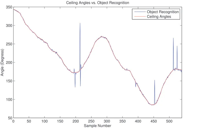
7 Ceiling Angles Method vs. Object Recognition . . . 28
8 Video Size Comparison . . . 29
9 Inertial Sensor vs. Ceiling Angles . . . 30
SR-2009-01
1
Summary
The purpose of this report is to document the optical systems developed during the Winter 2009 work term. These systems were developed for the purpose of determining the heading angle of a vessel under indoor test conditions to compliment the current Qualisys and inertial navigation systems for control purposes. Brief usage instructions are also included.
SR-2009-01
2
Introduction
When a model test takes place at the Institute for Ocean Technology, a control system is needed to navigate the vessel properly when an autopi-lot is implemented. This control system needs to know the heading of the vessel at all times in order to accurately control the vessel. Currently there are two methods used to measure the heading angle (among other pa-rameters), which are the non-contact optical Qualisys system and a yaw rate sensor. These systems, however, are not perfect. The advantages and disadvantages of these systems will be discussed, and several new ideas will be presented for measuring heading, including the light positions method, ceiling angles method, and the object recognition method.
SR-2009-01
3
Discussion
3.1
Qualisys
The Qualisys system is a non-contact optical system that uses infrared cameras and lights to capture reflective or active points on the vessel, and uses software to determine the position of the vessel. The main advantage of the Qualisys system is that it directly measures the vessel’s position and orientation resulting in a drift-free signal, unlike a yaw rate sensor. How-ever, the Qualisys system has its disadvantages. There is lack of coverage in some areas of the Offshore Engineering Basin (OEB), particularly the East side where both cameras cannot ”see” simultaneously. Also, there are occasional dropouts and unknown latency due to the multiple conver-sions and inconvenient hardware and software (1). While very accurate and drift-free, these downfalls make the Qualisys system unideal for real-time control purposes. Despite these downfalls, the ideas in this report are not meant to replace the Qualisys system, but compliment it. This is be-cause the Qualisys system has more to offer than just heading reference, it gives the complete position of the vessel.
3.2
Inertial Measurement Unit
When a model test is performed at IOT, an inertial measurement unit is usually mounted on the vessel to acquire data from the six degrees of
freedom (roll, pitch, yaw, surge, sway, and heave) for control and post processing purposes. The IMUs in this report may also be referred to as rate gyros or yaw rate sensors, since for the purpose of this project we are only looking at the yaw/turn rate from the IMU. Control systems use these IMUs by numerically integrating the yaw rate signal to give heading. Such IMUs include devices like the Crossbow IMU700, which is one of the most accurate fiber optic IMUs available. But even with a high-end device such as the Crossbow, drift is inevitable. Drift is caused by integrating the yaw rate signal as shown in Equation 1. ψ refers to the heading and ˙ψ refers to the yaw rate.
ψ(t) = Z
˙
ψ(t)dτ + ψof f s (1)
After each integration a new drift term is added to the previous values, accumulating over time. Because of this drift problem, an IMU alone is not very useful for control purposes. If both the IMU and an independent non-drifting signal are combined in a Kalman filter, however, a stabilized yaw can be produced. Currently the Qualisys system is functioning as that non-drifting signal, but because of the aforementioned problems, it is not ideal. The following are ideas to attempt to compliment the current heading reference devices.
SR-2009-01 3.3 Light Positions
3.3
Light Positions
One of the very first methods that was explored was the light position method. It is based on the basic idea of triangulation. If the positions of two points in space and the relative angles to an object are known, it is possible to determine the location of the object through trigonometry.(2)
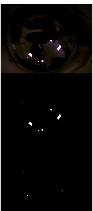
This light position method uses 3 or more lights or detectable points around the testing area (the OEB in the case of this project) and a cam-era that is able to view all of the lights, such as a 180-degree field of view fisheye lens, a rectilinear catadioptric lens, or a simple reflective sphere with a camera looking directly up or down at it. Software designed specif-ically for this purpose find and detect the lights and their relative angles. Through trigonometry a number of equations can be generated, and by using a system of equations algorithm it is possible to solve them for the position and rotation (heading) of the system. The main equation used is equation 2 where i is the light number, αi and βi are, respectively, the x-and y-coordinates of the lights in the test area, x-and x, y, x-and ψ are, re-spectively, the x- and y-coordinates and heading of the object. Θi are the angles of the lights measured in the image. For each light, a new equa-tion is created, and using a funcequa-tion called ”LMFnlsq” (located on MATLAB Central), one is able to solve the equations for x, y, and ψ.
0 = αi− x − (βi− y) tan (Θi+ ψ) (2) Figure 1 shows the steps involved in isolating the lights from the
surround-ing environment. This image was created in a semi-controlled environment so it was easy to obtain the desired results.
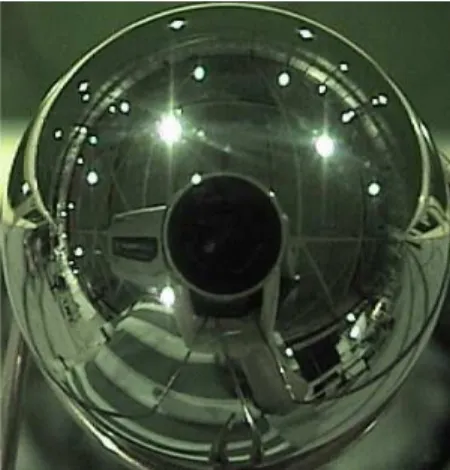
However, a couple of problems were encountered while testing the light position method. Firstly, if there was a dropout (one or more of the lights had not been captured), it’s nearly impossible to determine which light was dropped. This would confuse the software and ultimately end up in an er-ror. Secondly, as displayed in Figure 2 the numerous lights and reflections in the OEB were difficult to isolate from the lights needed for the system. The software continually picked up these lights and it often gave very in-accurate answers as a result. Because of these problems, it was decided that this method was not feasible to continue working on. One benefit of this method, however, was that it was possible to determine position as well as heading, while the following two methods only supply heading.
3.4
Ceiling Angles
The second explored method was the ceiling angles method. This involved placing a camera on the vessel looking up at the ceiling of the OEB. The camera would take pictures or video of the ceiling and software developed in MATLAB would analyze and edge detect the images, then determine the angle of one of the beams. This is accomplished by the fact that every beam in the OEB is oriented at either 0◦, 45◦, or 90◦. The software mea-sures the angle of either of the beams and converts it to an angle from 0◦
SR-2009-01 3.4 Ceiling Angles
Figure 1: From top to bottom: The image is taken, the software performs a
Figure 2: The OEB is unideal for the light position method
to 45◦. Once all of the angles have been collected from the sequence of pictures or video, it is ”unwrapped” to give a reading from 0◦ to 360◦ given an initial angle estimate.
Currently, the MATLAB software returns angles rounded to the nearest degree. In future applications it may be more accurate if several decimal places were used.
3.4.1 Usage
To use the ceiling angles method with a prerecorded video, run the function edgefinder2_vid.m under a MATLAB environment. There are two argu-ments: vidname, the file path of an AVI video is passed in, and init, an estimate of the initial angle. An array called fixangle is returned, which is the unwrapped data from 0◦ to 360◦. Also, in the second column is the
SR-2009-01 3.4 Ceiling Angles
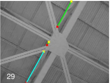
Figure 3: The prominent edges are located.
29
quadrant/octant the angle was in when it was unwrapped.
A similar function called edgefinder2_createvideo.m also returns a MATLAB video file called angvideo, which shows frame by frame which edge was detected. This may be useful for troubleshooting or presentation purposes. edgefinder2.m is just a script form of the other functions, meant to work with a directory of sequentially named image files.
3.5
Object Recognition
The third explored method was the object recognition method. This method is similar to the ceiling angles method in the fact that a camera is placed on the vessel looking at a ceiling. However for this method a known object, shape, or image is placed on the ceiling and the camera takes a succes-sion of pictures or video of the ceiling. Using an algorithm called SIFT (Scale-Invariant Feature Transform), software developed in MATLAB iden-tifies keypoints of each object (3). These keypoints are compared to those on the reference image to find an angle difference in between them, deter-mining the orientation of the object. That orientation is then translated to a heading angle.
Care has to be taken into account with regards to the surroundings, be-cause the SIFT algorithm will pick up keypoints from just about any object, not only the ones we are looking for. This is generally not a problem, but if the surroundings are too distracting, it greatly increases processing speed
SR-2009-01 3.5 Object Recognition
and error. One type of error occurs when a keypoint from the object is incorrectly matched to a keypoint on the reference image. Another type of error is when the image is almost exactly lined up with the reference image. In this case it has the tendency to pick up on an angle close to 0◦ and also close to 360◦. In some cases, it may take the average of both, giving an answer around 180◦. A way to solve this when this system is implemented on a vessel is to rotate the system 180◦. This is because during testing, a vessel rarely rotates past 180◦ and would not encounter this problem as often. It has also been noticed, however, that at 180◦ fewer SIFT points are matched than at another arbitrary angle (the reason for this is yet to be determined). ”Unwrapping” the data may also work for the purpose of preventing the jump from 0◦ to 360◦.
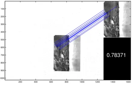
Some of the types of shapes that can be used on the ceiling should have a number of sharp corners and edges as opposed to rounded edges. For example a large printed ”F” or ”T” (as seen in Figure 5) would supply more SIFT points than an ”O” or ”C”. However it has been discovered that it’s not the shapes themselves that make a huge difference, images with more gradients/shades and complex scenes (i.e. a magazine cover or a picture of a city, as seen in Figure 6) are more recognizable to the SIFT algorithm. If an image contains repeating patterns it will incorrectly match keypoints, so it is best if the image is more organic or random.
Another shape recognition method that was recently explored is ASIFT (Affine Scale-Invariant Feature Transform or Affine-SIFT). SIFT uses zoom,
101.266 100 200 300 400 500 600 700 800 900 1000 50 100 150 200 250 300 350 400 450
Figure 5: Object recognition using an ’F’ shape.
0.78371 200 400 600 800 1000 1200 1400 1600 100 200 300 400 500 600 700 800 900 1000
SR-2009-01 3.5 Object Recognition
rotation and translation to identify keypoints, but ASIFT adds more param-eters to accommodate for camera axis orientation, matching keypoints at a camera angle of 36◦and even higher angles (4). ASIFT is generally able to find more keypoints in any given situation than SIFT, therefore it would be a welcome addition to this project in future applications.
3.5.1 Usage
To use the object recognition method, one needs the SIFT demo program located at http://www.cs.ubc.ca/ lowe/keypoints/. The video_run.m script uses the SIFT algorithm to work its way through each video frame and matches the object to the reference video. It creates the angle array. Un-comment A(:,i)=getframe(gca); to create a video of the function work-ing. The code with image = imresize(image,number) resize the refer-ence image and the video. Experiment with different numbers to get the best results. Lower numbers also equate to higher processing speed.
The match4.m function is a heavily modified function included in the SIFT demo program that returns the angle at which the object is rotated. At approximately line 61-62 there is a bounding box so as to only pick up one object at a time. Adjust the numbers to represent the width and height of the box in pixels.
The sift.m file included with the SIFT demo program is slightly mod-ified where the image = imread(imageFile); line is commented out so it is possible to pass in an actual image instead of the filepath of an image.
It is referred to as sift2.m.
3.6
Hardware
3.6.1 uEye Camera
The main camera used for this project is the uEye UI-2240RE-M-GL In-dustrial Camera. It is a USB 2.0 compatible camera with a resolution of 1280x1024 and a maximum full-size framerate of 15 frames per second. The software that is included with it (uEye Demo) allows the user to change all of it’s settings (i.e. exposure, framerate, gain, etc.) and also allowed the capture of video and still images. Because this software allowed for these functions it was not necessary (for this project) to integrate it directly into MATLAB, but it can be done.
Two lenses were ordered along with the camera as well. These are the Kowa LM12JCM and the Fujinon DF6HA-1B. The Kowa has a 12mm focal length and a maximum aperture of f/1.4 and the Fujinon has a 6mm focal length and a maximum aperture of f/1.2. Both lenses were sufficient for the project but the 6mm will probably be used more because of its wider field of view.
3.6.2 Analog Devices Inertial Sensor
The inertial sensor used to compare results and test the theory of this project was the Analog Devices ADIS16354AMLZ Inertial Sensor. It is
SR-2009-01 3.6 Hardware
a 6-axis sensor (roll, pitch, and yaw rate gyros, and heave, sway, and surge accelorometers). Power was supplied to the device through a USB cable and interfaced with a parallel port cable (IEEE 1284). The data was recorded on a Compaq Evo N410c notebook computer.
3.6.3 Canon A720IS
The Canon A720IS is a digital point and shoot camera used for the initial testing before the uEye camera was acquired. It is an 8.0 megapixel cam-era with 6x optical zoom. Videos were recorded on it, then transferred to the computer for analysis.
SR-2009-01
4
Conclusions
Two of the three ideas mentioned here have proved to be feasible options for recording the heading of a vessel under test conditions for both control and post-processing applications. While a fair amount of time was spent researching the light positions method, it has been determined that it will be very difficult to use in the OEB because of the distracting objects and lights. While both the ceiling angles and object recognition methods are very good, the object recognition seems to be the better choice for con-trol because an initial angle is not needed, but the ceiling angles method seem to be better for post-processing applications because of it’s greater consistency.
SR-2009-01
5
Recommendations
Both the ceiling angles and object recognition methods have room for im-provement. The ceiling angles method may be improved by having an algorithm that returns angles in doubles instead of just integers (i.e. 26.56 vs. 27). The object recognition method may be improved by exploring all the possible shape combinations for the SIFT keypoint recognition to de-termine which gives the most accurate results for this application. Each object could also be detected more intelligently as well to provide more keypoints.
For both of these methods, it would be ideal if one used a high resolu-tion camera with a semi-wide-angle lens with the lowest distorresolu-tion possible to achieve the most accurate results. Also, the higher the framerate, the more data points, and the less chance that the data will end up in the wrong quadrant when using the ceiling angles method.
SR-2009-01 REFERENCES
References
[1] J. Millan, G. Janes, and D. Millan, “Autopilot system for surface ma-noeuvring of a submarine,” Laboratory Memorandum LM-2008-06, In-stitute for Ocean Technology, 2009.
[2] Wikimedia Foundation, Triangulation, 2009. 20 April 2009.
[3] D. G. Lowe, “Distinctive image features from scale-invariant keypoints,”
International Journal of Computer Vision.
[4] J. Morel and G. Yu, “ASIFT: A new framework for fully affine invariant image comparison,” SIAM Journal on Imaging Sciences, 2009.
SR-2009-01
SR-2009-01
A
T
e
s
t
R
e
s
u
lt
s
0 0 9 -0 1 A T E S T R E S U LT 0 50 100 150 200 250 300 350 400 450 500 50 100 150 200 250 300 350 Sample Number Angle (Degress) Object Recognition Ceiling Angles
S R -2 0 0 9 -0 1 0 50 100 150 200 250 300 350 400 450 500 50 100 150 200 250 300 350 400 450 500 550 Sample Number Angle (Degress)
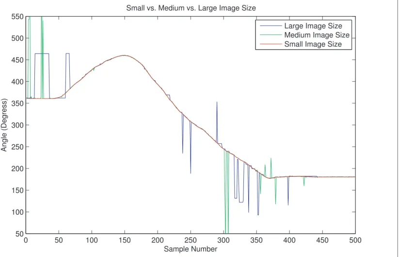
Small vs. Medium vs. Large Image Size
Large Image Size Medium Image Size Small Image Size
Figure 8: A comparison of using different resolutions for the Object Recognition method. Large (full size) is
1280x1024 pixels, Medium is 50%, and Small is 20%. Both the video and reference images have been resized.
2
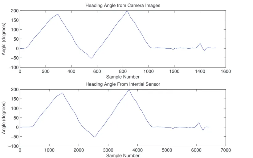
0 0 9 -0 1 A T E S T R E S U LT 0 200 400 600 800 1000 1200 1400 1600 −100 −50 0 50 100 150 200 Angle (degrees) Sample Number 0 1000 2000 3000 4000 5000 6000 7000 −100 −50 0 50 100 150 200 Sample Number Angle (degrees)
Heading Angle From Intertial Sensor
perspec-S R -2 0 0 9 -0 1 0 50 100 150 200 250 −6 −4 −2 0 2 4
Heading Angle from Camera Images
Sample Number Angle (degrees) 0 100 200 300 400 500 600 700 800 −8 −6 −4 −2 0 2
Heading Angle from Inertial Sensor
Sample Number
Angle (degrees)
Figure 10: A comparison between the ceiling angles method and the inertial sensor data. Clearly, the resolution
of the inertial sensor is much greater upon close inspection.
3
0 0 9 -0 1 B MA T L A B C O D
B.1
lightpositions.m
1 %%2 % Position locater for a visual tracking system 3 % Written by: AJ Smith
4 % Date: Feb 3 2009 5 % Updated: Feb 9 2009
6 % Requires the function LMFnlsq by M. Balda located on MATLAB Central
7 %%
8 % Take an image and get information on the location of lights 9 clear; 10 centerx = 295; 11 centery = 229; 12 I = imread('Picture 21.jpg'); 13 G = I(:,:,2); 14 %Th = (I(:,:,2)>140); 15 Th = im2bw(G,0.6); 16 [labeled,numObjects] = bwlabel(Th,8); 17 alldata = regionprops(labeled,'basic'); 18 j = 1; 19 for i = 1:numObjects 20 if alldata(i,1).Area < 20 21 lightdata(j,1) = alldata(i,1); 22 j = j+1; 23 end 24 end
S R -2 0 0 9 -0 1 B .1 lig h tp o s itio n s .m 27 for i = 1:j−1 28 angle = atan2(lightdata(i,1).Centroid(1)−centerx, ... 29 centery−lightdata(i,1).Centroid(2)); 30 if angle < 0
31 angle = angle + (2*pi);
32 end 33 lightangles(i,1) = angle; 34 end 35 sortangles = sort(lightangles); 36 37 %t = sortangles; 38 %for k = 0:offset 39 t = [sortangles(2); 40 sortangles(3); 41 sortangles(4); 42 sortangles(5); 43 sortangles(1);]; 44 %end 45 differences = diff(t) 46 47 %%
48 % Use a non−linear system of equations to determine position and heading 49 %a = [0;24;60;50;10]; %x−coordinates of lights 50 %b = [59;84;45;0;0]; %y−coordinates of lights 51 52 a = [50;47;0 ;24;60]; %x−coordinates of lights 53 b = [0 ; 0;59;84;45]; %y−coordinates of lights 54
55 x0 = [0;0;0]; %initial guess of position 56
57
58 ffun = @(x) [a(1)− x(1)−(b(1)−x(2))*tan(x(3)+t(1));
3
0 0 9 -0 1 B MA T L A B C O D 60 a(3)− x(1)−(b(3)−x(2))*tan(x(3)+t(3)); 61 a(4)− x(1)−(b(4)−x(2))*tan(x(3)+t(4)); 62 a(5)− x(1)−(b(5)−x(2))*tan(x(3)+t(5))]; 63 64 LMFnlsq(ffun,x0) 65 66 67 %% 68 q = zeros(480,640); 69 for i = 1:5 70 q(int16(lightdata(i,1).Centroid(2)), ... 71 int16(lightdata(i,1).Centroid(1))) = 255; 72 end 73 %figure,imshow(q)
S R -2 0 0 9 -0 1 B .2 lig h tp o s itio n s 2 .m
B.2
lightpositions2.m
1 %%2 % Position locater for a visual tracking system 3 % Written by: AJ Smith
4 % Date: Feb 3 2009 5 % Updated: Feb 13 2009
6 %%
7 % Take an image and get information on the location of lights 8 clear; 9 centerx = 295; 10 centery = 229; 11 I = imread('Picture 19.jpg'); 12 G = I(:,:,2); 13 %Th = (I(:,:,2)>140); 14 Th = im2bw(G,0.6); 15 [labeled,numObjects] = bwlabel(Th,8); 16 alldata = regionprops(labeled,'basic'); 17 j = 1; 18 for i = 1:numObjects 19 if alldata(i,1).Area < 20 20 lightdata(j,1) = alldata(i,1); 21 j = j+1; 22 end 23 end 24 %%
25 % Find the angles of the lights 26 for i = 1:j−1
27 angle = atan2(lightdata(i,1).Centroid(1)−centerx, ... 28 centery−lightdata(i,1).Centroid(2));
3
0 0 9 -0 1 B MA T L A B C O D
30 angle = angle + (2*pi);
31 end
32 lightangles(i,1) = angle;
33 end
34 sortangles = sort(lightangles); 35
36 % the following code sorts the angles of the points
37 % the two points with the smallest angle between each other 38 % are the reference points
39 differences = diff(sortangles); 40 min diff = 10;
41 for i = 1:size(differences) 42 if min diff > differences(i) 43 min diff = differences(i); 44 offset = i−1; 45 end 46 end 47 48 49 for k = 1:offset 50 sortangles = [sortangles(2); 51 sortangles(3); 52 sortangles(4); 53 sortangles(5); 54 sortangles(1);]; 55 end 56 %differences = diff(t) 57 t = sortangles; 58 59 %%
S R -2 0 0 9 -0 1 B .2 lig h tp o s itio n s 2 .m 61 %a = [0;24;60;50;10]; %x−coordinates of lights 62 %b = [59;84;45;0;0]; %y−coordinates of lights 63 64 a = [50;47;0 ;24;60]; %x−coordinates of lights 65 b = [0 ; 0;59;84;45]; %y−coordinates of lights 66
67 x0 = [0;0;0]; %initial guess of position 68
69
70 ffun = @(x) [a(1)− x(1)−(b(1)−x(2))*tan(x(3)+t(1)); 71 a(2)− x(1)−(b(2)−x(2))*tan(x(3)+t(2)); 72 a(3)− x(1)−(b(3)−x(2))*tan(x(3)+t(3)); 73 a(4)− x(1)−(b(4)−x(2))*tan(x(3)+t(4)); 74 a(5)− x(1)−(b(5)−x(2))*tan(x(3)+t(5))]; 75 76 LMFnlsq(ffun,x0) 77 78 79 %%
80 % plot the assumed positions of the lights 81 q = zeros(480,640); 82 for i = 1:5 83 q(int16(lightdata(i,1).Centroid(2)), ... 84 int16(lightdata(i,1).Centroid(1))) = 255; 85 end 86 figure,imshow(q) 3 7
S R -2 0 0 9 -0 1 B .3 e d g e fi n d e r2 .m
B.3
edgefinder2.m
1 % sorts through a folder of images and finds the angles of edges in each 2 % image, adding it to the angles[] array.
3 % returns the array [fixangle] containing the angles and quadrants 4 % corresponding to the angle.
5 % function [angles] = edgefinder2(init)
6 %
7 % Created Feb 10 2009 8 % A. Smith
9 %
10 images = dir('image2/*.jpg'); 11 for i = 1:size(images)
12 rgb img = imread(strcat('image2/',images(i).name)); 13 I = rgb img(:,:,1);
14 BW = edge(I,'canny',0.3); 15 [H,theta,rho] = hough(BW);
16 P = houghpeaks(H,1,'threshold',ceil(0.3*max(H(:)))); 17 x = theta(P(:,2));
18 y = rho(P(:,1)); 19
20 % The following code converts the angle found to an angle between 0 and 21 % 45 degrees, because the ceiling in the Offshore Engineering Basin has 22 % 3 angles: 0, 45, and 90 degrees. This way it doesn't matter which one 23 % the edge detection picks up.
24 if x ≥ −90 && x < −45 25 angle = x+90 26 elseif x ≥ −45 && x < 0 27 angle = x+45 28 elseif x > 45 && x < 90 3 9
0 0 9 -0 1 B MA T L A B C O D 30 else 31 angle = x 32 end 33 angles(i) = angle; 34 end 35
36 %% Go through the array of angles and "unwrap" it from 0−45 to 0−360 37 % Determine what "quadrant" (technically octant) the initial angle is in 38 init = 359; % initial estimate of the first angle
39 if init ≥ 0 && init < 45 40 quadr = 1;
41 elseif init ≥ 45 && init < 90
42 quadr = 2;
43 elseif init ≥ 90 && init < 135
44 quadr = 3;
45 elseif init ≥ 135 && init < 180
46 quadr = 4;
47 elseif init ≥ 180 && init < 225
48 quadr = 5;
49 elseif init ≥ 225 && init < 270
50 quadr = 6;
51 elseif init ≥ 270 && init < 315
52 quadr = 7;
53 elseif init ≥ 315 && init < 360
54 quadr = 8;
55 else
56 quadr = 0;
57 end
58
S R -2 0 0 9 -0 1 B .3 e d g e fi n d e r2 .m 61 switch quadr 62 case 1 63 angle = angles(i); 64 case 2 65 angle = 45 + angles(i); 66 case 3 67 angle = 90 + angles(i); 68 case 4 69 angle = 135 + angles(i); 70 case 5 71 angle = 180 + angles(i); 72 case 6 73 angle = 225 + angles(i); 74 case 7 75 angle = 270 + angles(i); 76 case 8 77 angle = 315 + angles(i); 78 end 79 fixangle(1,i) = angle; 80 % fixangle(2,i) = quadr;
81 diffang = angles(i+1) − angles(i);
82 if diffang < −15 % detect when data crosses over to the next quadrant 83 if quadr == 8
84 quadr = 1;
85 else
86 quadr = quadr + 1;
87 end
88 elseif diffang > 15 % detect when data crosses back to the previous quadrant
89 if quadr == 1 90 quadr = 8; 91 else 92 quadr = quadr − 1; 4 1
3 e n d 4 e n d 5 e n d
S R -2 0 0 9 -0 1 B .4 e d g e fi n d e r2 v id .m
B.4
edgefinder2 vid.m
1 % function [fixangle] = edgefinder2 vid(vidname,init)
2 % vidname = a string "pointing" to an avi file, for example 'video.avi' 3 % init = the initial angle at which the data starts at
4 %
5 % returns the array [fixangle] containing the angles and quadrants 6 % corresponding to the angle.
7 %
8 % Created Feb 10 2009 9 % A. Smith
10 %
11 function [fixangle] = edgefinder2 vid(vidname,init)
12 vid = mmreader(vidname);
13 for i = 1:vid.NumberOfFrames−1 14 rgb img = read(vid,i);
15 bw img = rgb img(:,:,1); %edge function only accepts b&w images 16 %crops edge artifacts from frame
17 I = imcrop(bw img,[1 1 (size(bw img,2)−2) (size(bw img,1)−2)]); 18 BW = edge(I,'canny',0.3); %find all apparent edges
19 [H,theta,rho] = hough(BW);
20 P = houghpeaks(H,1,'threshold',ceil(0.3*max(H(:)))); 21 x = theta(P(:,2));
22 y = rho(P(:,1)); 23
24 % The following code converts the angle found to an angle between 0 and 25 % 45 degrees, because the ceiling in the Offshore Engineering Basin has 26 % 3 angles: 0, 45, and 90 degrees. This way it doesn't matter which one 27 % the edge detection picks up.
28 if x ≥ −90 && x < −45
4
0 0 9 -0 1 B MA T L A B C O D 30 elseif x −45 && x < 0 31 angle = x+45 32 elseif x > 45 && x < 90 33 angle = x−45 34 else 35 angle = x 36 end 37 angles(i) = angle; 38 end 39
40 %% Go through the array of angles and "unwrap" it from 0−45 to 0−360 41 %init = 100;
42 % Determine what "quadrant" (technically octant) the initial angle is in 43 if init ≥ 0 && init < 45
44 quadr = 1;
45 elseif init ≥ 45 && init < 90
46 quadr = 2;
47 elseif init ≥ 90 && init < 135
48 quadr = 3;
49 elseif init ≥ 135 && init < 180
50 quadr = 4;
51 elseif init ≥ 180 && init < 225
52 quadr = 5;
53 elseif init ≥ 225 && init < 270
54 quadr = 6;
55 elseif init ≥ 270 && init < 315
56 quadr = 7;
57 elseif init ≥ 315 && init < 360
58 quadr = 8;
S R -2 0 0 9 -0 1 B .4 e d g e fi n d e r2 v id .m 61 end 62
63 % Based on the inital angle, unwrap the data 64 for i = 1:(size(angles,2)−1) 65 switch quadr 66 case 1 67 angle = angles(i); 68 case 2 69 angle = 45 + angles(i); 70 case 3 71 angle = 90 + angles(i); 72 case 4 73 angle = 135 + angles(i); 74 case 5 75 angle = 180 + angles(i); 76 case 6 77 angle = 225 + angles(i); 78 case 7 79 angle = 270 + angles(i); 80 case 8 81 angle = 315 + angles(i); 82 end 83 fixangle(1,i) = angle; 84 fixangle(2,i) = quadr;
85 diffang = angles(i+1) − angles(i);
86 if diffang < −15 % detect when data crosses over to the next quadrant 87 if quadr == 8
88 quadr = 1;
89 else
90 quadr = quadr + 1;
91 end
92 elseif diffang > 15 % detect when data crosses back to the previous quadrant
4
0 0 9 -0 1 B MA T L A B C O D 94 quadr = 8; 95 else 96 quadr = quadr − 1; 97 end 98 end 99 end
S R -2 0 0 9 -0 1 B .5 e d g e fi n d e r2 c re a te v id e o .m
B.5
edgefinder2 createvideo.m
1 % function [fixangle] = edgefinder2 vid(vidname,init)
2 % vidname = a string "pointing" to an avi file, for example 'video.avi' 3 % init = the initial angle at which the data starts at
4 %
5 % returns the array [fixangle] containing the angles and quadrants 6 % corresponding to the angle.
7 %
8 function [fixangle,angvideo] = edgefinder createvideo(vidname,init)
9 vid = mmreader(vidname); 10 fig1 = figure(1); 11 % winsize = get(fig1,'Position') 12 % winsize(1:4) = [84 57 320 240] 13 for i = 1:500 %vid.NumberOfFrames−1 14 rgb img = read(vid,i);
15 bw img = rgb img(:,:,1); %edge function only accepts b&w images 16 %crops edge artifacts from frame
17 I = imcrop(bw img,[1 1 (size(bw img,2)−2) (size(bw img,1)−2)]); 18 BW = edge(I,'canny',0.3); %find all apparent edges
19 [H,theta,rho] = hough(BW);
20 P = houghpeaks(H,1,'threshold',ceil(0.3*max(H(:)))); 21 x = theta(P(:,2));
22 y = rho(P(:,1)); 23
24 %plot a figure showing the edges with the longest line highlighted 25 plot(x,y,'s','color','black');
26 lines = houghlines(BW,theta,rho,P,'FillGap',5,'MinLength',7); 27 imshow(I), hold on
28 max len = 0;
4
0 0 9 -0 1 B MA T L A B C O D 30 xy = [lines(k).point1; lines(k).point2];
31 plot(xy(:,1),xy(:,2),'LineWidth',2,'Color','green'); 32
33 % Plot beginnings and ends of lines
34 plot(xy(1,1),xy(1,2),'x','LineWidth',2,'Color','yellow'); 35 plot(xy(2,1),xy(2,2),'x','LineWidth',2,'Color','red'); 36
37 % Determine the endpoints of the longest line segment 38 len = norm(lines(k).point1 − lines(k).point2);
39 if ( len > max len) 40 max len = len; 41 xy long = xy;
42 end
43 end
44
45 % highlight the longest line segment
46 plot(xy long(:,1),xy long(:,2),'LineWidth',2,'Color','cyan'); 47
48 %A(:,i)=getframe(fig1,winsize); 49
50
51 % The following code converts the angle found to an angle between 0 and 52 % 45 degrees, because the ceiling in the Offshore Engineering Basin has 53 % 3 angles: 0, 45, and 90 degrees. This way it doesn't matter which one 54 % the edge detection picks up.
55 if x ≥ −90 && x < −45 56 angle = x+90
57 elseif x ≥ −45 && x < 0
58 angle = x+45
S R -2 0 0 9 -0 1 B .5 e d g e fi n d e r2 c re a te v id e o .m 61 else 62 angle = x 63 end 64 angles(i) = angle; 65
66 text(20,220,num2str(angle),'color','white','fontsize',16); 67 A(:,i)=getframe(gca);
68
69 end
70
71 %% Go through the array of angles and "unwrap" it from 0−45 to 0−360 72 %init = 100;
73 % Determine what "quadrant" (technically octant) the initial angle is in 74 if init ≥ 0 && init < 45
75 quadr = 1;
76 elseif init ≥ 45 && init < 90
77 quadr = 2;
78 elseif init ≥ 90 && init < 135
79 quadr = 3;
80 elseif init ≥ 135 && init < 180
81 quadr = 4;
82 elseif init ≥ 180 && init < 225
83 quadr = 5;
84 elseif init ≥ 225 && init < 270
85 quadr = 6;
86 elseif init ≥ 270 && init < 315
87 quadr = 7;
88 elseif init ≥ 315 && init < 360
89 quadr = 8; 90 else 91 quadr = 0; 92 end 4 9
0 0 9 -0 1 B MA T L A B C O D
94 % Based on the inital angle, unwrap the data 95 for i = 1:(size(angles,2)−1) 96 switch quadr 97 case 1 98 angle = angles(i); 99 case 2 100 angle = 45 + angles(i); 101 case 3 102 angle = 90 + angles(i); 103 case 4 104 angle = 135 + angles(i); 105 case 5 106 angle = 180 + angles(i); 107 case 6 108 angle = 225 + angles(i); 109 case 7 110 angle = 270 + angles(i); 111 case 8 112 angle = 315 + angles(i); 113 end 114 fixangle(1,i) = angle; 115 fixangle(2,i) = quadr;
116 diffang = angles(i+1) − angles(i);
117 if diffang < −15 % detect when data crosses over to the next quadrant 118 if quadr == 8
119 quadr = 1;
120 else
121 quadr = quadr + 1;
122 end
S R -2 0 0 9 -0 1 B .5 e d g e fi n d e r2 c re a te v id e o .m 125 quadr = 8; 126 else 127 quadr = quadr − 1; 128 end 129 end 130 end 131 angvideo = A; 5 1
S R -2 0 0 9 -0 1 B .6 v id e o ru n .m
B.6
video run.m
1 % A script to run through each frame in a video to determine it's
2 % orientation with respect to a reference image using the SIFT algorithm. 3 % Created by AJ Smith, March 2009
4 clear
5 vid = mmreader('video.avi');
6 F = imread('reference image.pgm');
7 % F = imresize(F,0.2); %resize the reference image 8 [im2, des2, loc2] = sift2(F);
9 for i = 1:vid.NumberOfFrames 10 rgb img = read(vid,i); 11 bw img = rgb img(:,:,1);
12 bw img = imresize(bw img,0.5); %resize the video frame
13 try
14 angle(i) = match4(bw img, im2, des2, loc2);
15 catch % if no angles are returned, duplicate the previous angle
16 if i > 1 17 angle(i) = angle(i−1); 18 else 19 angle(i) = 0; 20 end 21 end 22 i
23 % A(:,i)=getframe(gca); %create a MATLAB video
24 end 25 26 %% 27 % for i = 1:size(angle,2) 28 % if angle(i) <0 5 3
0 0 9 -0 1 B MA T L A B C O D 30 % end 31 % end
S R -2 0 0 9 -0 1 B .7 ma tc h 4 .m
B.7
match4.m
1 % num = match3(image1, image2)
2 %
3 % This function reads two images, finds their SIFT features, and
4 % displays lines connecting the matched keypoints. A match is accepted 5 % only if its distance is less than distRatio times the distance to the 6 % second closest match.
7 % It returns the angle at which the object in image2 is rotated compared to image1
8 %
9 % Example:
10 % orig = imload
11 % match('scene.pgm','book.pgm'); 12
13 function angle = match3(image1, im2, des2, loc2)
14
15 % Find SIFT keypoints for each image 16 [im1, des1, loc1] = sift2(image1); 17 %[im2, des2, loc2] = sift2(image2); 18
19 % For efficiency in Matlab, it is cheaper to compute dot products between 20 % unit vectors rather than Euclidean distances. Note that the ratio of 21 % angles (acos of dot products of unit vectors) is a close approximation 22 % to the ratio of Euclidean distances for small angles.
23 %
24 % distRatio: Only keep matches in which the ratio of vector angles from the 25 % nearest to second nearest neighbor is less than distRatio.
26 distRatio = 0.7; 27
28 % For each descriptor in the first image, select its match to second image.
5
0 0 9 -0 1 B MA T L A B C O D 30 for i = 1 : size(des1,1)
31 dotprods = des1(i,:) * des2t; % Computes vector of dot products 32 [vals,indx] = sort(acos(dotprods)); % Take inverse cosine and sort results 33
34 % Check if nearest neighbor has angle less than distRatio times 2nd. 35 if (vals(1) < distRatio * vals(2))
36 match(i) = indx(1); 37 else 38 match(i) = 0; 39 end 40 end 41
42 % Create a new image showing the two images side by side. 43 im3 = appendimages(im1,im2);
44
45 % Show a figure with lines joining the accepted matches. 46 %figure('Position', [100 100 size(im3,2) size(im3,1)]); 47 colormap('gray');
48 imagesc(im3);
49 %rect = [5 50 1345 590]; 50 rect = [5 50 1000 600]; 51 fig1 = figure(1);
52 set(fig1,'Position',rect); 53 hold on;
54 cols1 = size(im1,2); 55 count = 0;
56 for i = 1: size(des1,1) 57 if (match(i) > 0)
58 % Create a bounding box (so as not to select two objects) 59 % Adjust the numbers to accomodate for different image
S R -2 0 0 9 -0 1 B .7 ma tc h 4 .m
61 if ((loc1(i,1) < loc1(1,1)+90) && (loc1(i,1) > loc1(1,1)−90) &&... 62 (loc1(i,2) < loc1(1,2)+90) && (loc1(i,2) > loc1(1,2)−90)) 63 % draw lines between matching points
64 % line([loc1(i,2) loc2(match(i),2)+cols1], ... 65 % [loc1(i,1) loc2(match(i),1)], 'Color', 'c'); 66 count = count + 1;
67 x(count,1) = loc1(i,2); % first x−coordinate 68 x(count,2) = loc1(i,1); % first y−coordinate
69 x(count,3) = loc2(match(i),2)+cols1; % second x−coordinate 70 x(count,4) = loc2(match(i),1); % second y−coordinate
71 end 72 end 73 end 74 x = sortrows(x); 75 %x1,x2,y1,y2 76 count2 = 0; 77 for j = 1:count−1 78 if x(j,1)>(x(j+1,1)+3) | | x(j,1)<(x(j+1,1)−3) 79 % x(j,1),j 80 count2 = count2 + 1; 81 angle1 = atan2(x(j,2)−x(j+1,2), x(j,1)−x(j+1,1)); 82 angle2 = atan2(x(j,4)−x(j+1,4), x(j,3)−x(j+1,3)); 83 rot(count2) = (angle1−angle2)*180/pi;
84 if rot(count2) < 0 85 rot(count2) = rot(count2)+360; 86 end 87 88 line([x(j,1) x(j,3)], [x(j,2) x(j,4)]); 89 end 90 end 91 sort(rot) 92 angle = median(rot); 5 7
0 0 9 -0 1 B MA T L A B C O D 94 hold off; 95 %num = sum(match > 0);
S R -2 0 0 9 -0 1 B .8 s ift 2 .m
B.8
sift2.m
1 % [image, descriptors, locs] = sift(imageFile)
2 %
3 % This function reads an image and returns its SIFT keypoints. 4 % Input parameters:
5 % imageFile: the file name for the image.
6 %
7 % Returned:
8 % image: the image array in double format
9 % descriptors: a K−by−128 matrix, where each row gives an invariant 10 % descriptor for one of the K keypoints. The descriptor is a vector 11 % of 128 values normalized to unit length.
12 % locs: K−by−4 matrix, in which each row has the 4 values for a 13 % keypoint location (row, column, scale, orientation). The 14 % orientation is in the range [−PI, PI] radians.
15 %
16 % Credits: Thanks for initial version of this program to D. Alvaro and 17 % J.J. Guerrero, Universidad de Zaragoza (modified by D. Lowe) 18
19 function [image, descriptors, locs] = sift(image)
20
21 % Load image
22 %image = imread(imageFile); 23
24 % If you have the Image Processing Toolbox, you can uncomment the following 25 % lines to allow input of color images, which will be converted to grayscale. 26 % if isrgb(image)
27 % image = rgb2gray(image); 28 % end
5
0 0 9 -0 1 B MA T L A B C O D
30 [rows, cols] = size(image); 31
32 % Convert into PGM imagefile, readable by "keypoints" executable 33 f = fopen('tmp.pgm', 'w');
34 if f == −1
35 error('Could not create file tmp.pgm.');
36 end
37 fprintf(f, 'P5\n%d\n%d\n255\n', cols, rows); 38 fwrite(f, image', 'uint8');
39 fclose(f); 40
41 % Call keypoints executable 42 if isunix
43 command = '!./sift ';
44 else
45 command = '!siftWin32 ';
46 end
47 command = [command ' <tmp.pgm >tmp.key']; 48 eval(command);
49
50 % Open tmp.key and check its header 51 g = fopen('tmp.key', 'r');
52 if g == −1
53 error('Could not open file tmp.key.');
54 end
55 [header, count] = fscanf(g, '%d %d', [1 2]); 56 if count 6= 2
57 error('Invalid keypoint file beginning.');
58 end
S R -2 0 0 9 -0 1 B .8 s ift 2 .m 61 if len 6= 128
62 error('Keypoint descriptor length invalid (should be 128).');
63 end
64
65 % Creates the two output matrices (use known size for efficiency) 66 locs = double(zeros(num, 4));
67 descriptors = double(zeros(num, 128)); 68
69 % Parse tmp.key 70 for i = 1:num
71 [vector, count] = fscanf(g, '%f %f %f %f', [1 4]); %row col scale ori 72 if count 6= 4
73 error('Invalid keypoint file format');
74 end
75 locs(i, :) = vector(1, :); 76
77 [descrip, count] = fscanf(g, '%d', [1 len]); 78 if (count 6= 128)
79 error('Invalid keypoint file value.');
80 end
81 % Normalize each input vector to unit length 82 descrip = descrip / sqrt(sum(descrip.ˆ2)); 83 descriptors(i, :) = descrip(1, :);
84 end
85 fclose(g);
6