Bio-inspired swimming helix

A~C~UE.$

Bio-Inspired Swimming Helix

by

Benjamin C. F. Johnson

S.B. Electrical Engineering and Computer Science, MIT 2010

Submitted to the Department of Electrical Engineering and Computer

Science

in Partial Fulfillment of the Requirements for the Degree of

Masters of Engineering in Electrical Engineering and Computer

Science

at the Massachusetts Institute of Technology

May 2012

@

Massachusetts Institute of Technology 2012. All rights reserved.

Author..

Diartment of Eltical Engineering and Computer Science

May 21, 2012

C ertified by ...

Alexandra H. Techet, Associate Professor, Thesis Supervisor

May 21, 2012

K

Accepted by... ...

..

..

...

Prof. Dennis M. Freeman,

Chairman, Masters of Engineering Thesis Committee

Bio-Inspired Swimming Helix

by

Benjamin C. F. Johnson

Submitted to the Department of Electrical Engineering and Computer Science on May 21, 2012, in Partial Fulfillment of the

Requirements for the Degree of

Masters of Engineering in Electrical Engineering and Computer Science

Abstract

This thesis investigated a bio-inspired swimming chain (BISH), inspired by Weelia

cylindrica. After developing a model, it was used to investigate conditions under

which helical motion would emerge. The properties of this chain as the number of nodes changes was also investigated, to see if the helical motion or other properties of its motion were emergent behaviors. Other modes of motion were also observed. Optimization of the angle of propulsion of each was performed, and other optimiza-tions attempted, although practical difficulties prevented useful results. A ten node chain was constructed to empirically verify the helical mode of motion.

Thesis Supervisor: Alexandra H. Techet Title: Associate Professor

Contents

1 Introduction 11 1.1 Bio-inspiration . . . . 11 1.2 Salps . . . . 11 1.3 Underactuated Systems. . . . . 12 1.4 Motivation . . . . 14

2 Modeling and Simulation 15 2.1 Introduction . . . . 15 2.2 Model ... .. ... 15 2.2.1 Drag . . . . 16 2.2.2 Bouyancy . . . . 17 2.2.3 Node Connections. . . . . 18 2.2.4 Propulsion . . . . 18 2.3 Simulation . . . . 19

2.4 Model issues and Practical considerations . . . . 20

2.5 Modes of Motion . . . . 21

2.6 Model Validation . . . . 25

3 Optimization 27 3.1 Introduction . . . . 27

3.2 Stochastic Gradient Search. . . . . 27

3.3 Results. . . . . 29

3.3.2 Optimization issues and incomplete/failed attempts . . . . 29

3.3.3 Conclusions and Suggestions for Improvements . . . . 31

4 Contraction and Stability Analysis 33 4.1 Introduction . . . . 33

4.2 Dynamic Equations . . . . 34

4.2.1 Variable Descriptions . . . . 34

4.2.2 Equation for a Single Node . . . . 34

4.3 Initial Attempt at Contraction Analysis: Coupling Terms . . . . 35

4.4 Contraction Analysis: The Jacobian . . . . 36

4.5 Emergent Behavior . . . . 39

5 Physical Implementation 41 6 Conclusion and Suggestions for Future Work 45 A Derivation of Equations for Single Node 47 A.1 Variable Descriptions . . . . 47

B Paramters for BISH simulations 51 B.1 Parameters for Propulsion Angle Optimization . . . . 51

List of Figures

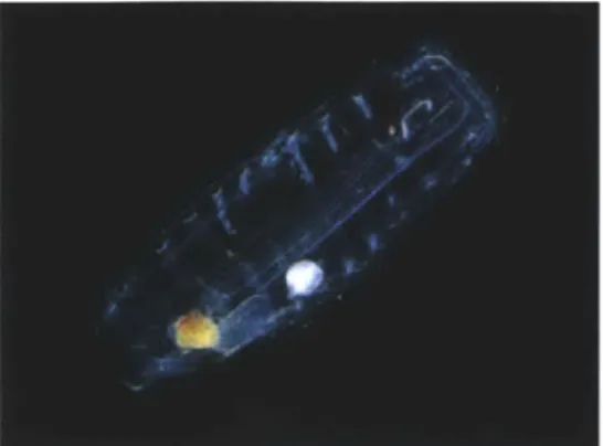
1-1 A single zooid of Weelia cylindrica. . . . . 12

1-2 The solitary and aggregate forms of three salp species[6]. . . . . 13

1-3 Weelia cylindrica in its aggregate form, swimming in a helix [8]. . . . 13

2-1 The body coordinates used for each node. . . . . 16

2-2 A Drawing showing Weelia Cylindrica in its aggregate chain form. Arrows indicate direction of fluid flow [6]. . . . . 19

2-3 The time to simulate the BISH model as a function of number of nodes in the chain. . . . . 21

2-4 Example of center of mass motion during helical motion. . . . . 23

2-5 The x component of the center of mass velocities in the inertial frame of a chain moving in a helix along a helical trajectory. . . . . 23

3-1 All points visited by stochastic gradient while searching for the optimal propulsion angle. . . . . 30

3-2 Results of 50 runs of propulsion angle optimization. Showing that many times the simulations necessary halt due to errors. All the red dots at the bottom halted on the first iterations of the optimization. . 30 4-1 Parameters of helical motion as a function of number of nodes in the chain. . . . . 40

5-1 A single node of the BISH and its neighbors . . . . 42

5-2 The BISH in a typical configuration . . . . 42

List of Tables

Chapter 1

Introduction

1.1

Bio-inspiration

Biological systems function and act in ways often very different from human-engineered

systems. Recently there has been a growing trend in imitating and finding inspiration

in nature for novel and better engineered systems. This includes all sorts of

technolo-gies from an efficient bio-inspired analog to digital converter

[11]

to robotic fish that

seek to emulate some of the hydrodynamic efficiencies of real fish, such as RoboTuna

[1]. Many mechanisms in nature are under-actuated, which may contribute to their

efficiency. In this project and many others, there is a hope to gain insights into how

biological creatures work and why they have the mechanisms they do. In this thesis

I investigate how the salp Weelia cylindrica is able to swim in a helical shape.

1.2

Salps

Salps are gelatinous underwater creatures, usually cylindrical in shape [3], which

squirt water out their rear orifice to propel themselves. During on part of their life

cycle salps exist as solitary organisms, like the one in Figure 1-1. In the part of

their life cycle, salps are born as aggregates of various morphologies depending on

their species [3]. Figure 1-2 shows a few examples. Weelia cylindrica, also known as

Figure 1-1: A single zooid of Weelia cylindrica.

helixes as they swim through the water. Figure 1-3 shows a picture of one swimming

in the ocean. This helical shape is interesting and slightly puzzling because there are

no muscles between the individual salps (zooids) nor anything rigid to give them this

shape. Because of this lack of actuation, Weelia cylindrica in its aggregate form can

be modeled as an underactuated system; these systems are an area of active research

in robotics.

1.3

Underactuated Systems

The differential equations for almost all robotic systems can be written in the form

[9]:

4 = fi(q, el, t) + f2(q, el, t)u.

(1.1)

When rank[f

2

(q, 4, t)u] < dim[q] the system is under-actuated. An intuitive way of

understanding this is that a system is under actuated if it is not possible for the control

input, u, to create an instantaneous acceleration in any direction. The column space

of f

2

does not span R' where n

=

dim[q]. A simple example of this occurs when there

are more degrees of freedom than there are actuators. Underactuated mechanisms

are an active area of research in robotics. Many standard control formulations and

approaches cannot be directly applied to these situations.

B. Pegs. conftednt aggrsg

Stolon

C. Ieha (Salu) eynches slty

F Cybse sew* ap egate

Figure 1-2:

The solitary and aggregate forms of three salp species[6].

Figure 1-3: Weelia cylindrica in its aggregate form, swimming in a helix [8].

1.4

Motivation

Weelia cylindrica in its aggregate form is underactuated, assuming at least one

addi-tional degree of freedom for for the chain for each salp. In addition it only has muscles

for propulsion cite, no muscles or rigid parts to control the shape of the aggregate.

Despite these factors it forms a helical structure as it swims, shown in Figure 1-3. The

question of how it does this appealed to me and was investigated primarily through a

series of simulations and optimizations, with some of the basic ideas being confirmed

by the construction of a ten node chain. Inspired by these salps, I modeled and built

a chain where each node was analogous to a single salp, having its own propulsion

and being coupled to its neighbors.

Chapter 2

Modeling and Simulation

2.1

Introduction

This section describes the model and and simulation of the salp inspired under-actuated swimming chain. The chain is modeled as rigid nodes connected by pivot joints. This was chosen because a rigid model like this is easier to analyze both in

simulation and analytically. I implemented it with SimMechanics Toolbox in Matlab. This was utilized because of the ability to model the system without having to explic-itly write out the differential equations. Appendix A contains the derivation of the equations of motion for a single node; however, the equations of motion for an entire chain were deemed too complex to be useful. Matlab was then used to numerically simulate this model, to look at the chains dynamic behavior.

2.2

Model

Each node was modeled as an elliptical rigid body connected to its neighbors by two rotational degrees of freedom. The propulsion was modeled as a force and torque acting on a particle point on each rigid body.

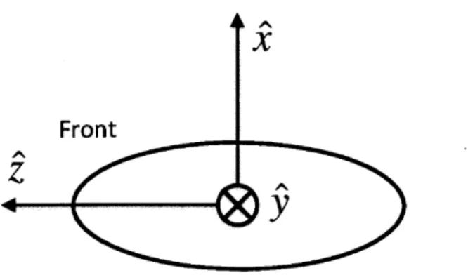
Euler angles were used to describe the rotation of each node. The z-y-x convention was used, meaning to go from the world coordinate reference frame first rotate

4

about the z axis, then 0 about the resulting intermediate y-axis then V) about the resulting

Front

X

Figure 2-1: The body coordinates used for each node.

x-axis, which is the body-fixed coordinate frame x-axis. The body fixed coordinates are shown in Figure 2-1. Transforming a vector from global coordinates to local coordinates then takes the form:

Vlocal = RxRyRzvgobai. (2.1)

Sign conventions must be observed since opposite signs are used for the angles when converting vectors between reference frames as opposed to rotating a reference frame to its position relative to the world coordinates.

2.2.1

Drag

Hydrodynamic drag was modeled as v2 drag, where v is velocity. The constants for the different cardinal directions were constant multiples of each other corresponding to the different surface areas. The drag for each node was calculated independently during the simulation, based only on equations 2.2 and 2.3. This means streamlining and drafting affects are not taken into account at all in this model. This is one significant difference between the BISH (Bio-Inspired Swimming Helix) that is modeled and

Weelia cylindrica. The chain structure of w. cylindrica greatly reduces the drag

Translational drag equation with components in the axis of the local frame:

FD=

ICy~IjI

(2.2)

Rotational drag equation with components in the axis of the local frame:

[bxw w.

Il

TD =-bywyIwyI

(2.3)

[b~w.

I w.

I

The drag forces and torques were applied to the center of pressure of the body. The center of pressure was one of the parameters of the model. It was always chosen to be some length behind the center of mass on the z-axis.

The close relationship between force, velocity, and drag contributed to the stiffness of the system. For this reason in the model, the drag force was applied to an extra rigid body, 100 times smaller then the node, and their center of masses were attached

by six springs and dampers, with very high spring constants. The spring constants

were high enough that the time constant of the small mass and the springs was much faster then everything else going on, and the deflections small enough so they would not perturb the results to any noticeable extent. This significantly speeded up the simulation times, by loosening the coupling between these terms.

2.2.2

Bouyancy

The model did not account for buoyancy or gravity at all. This is equivalent to assuming the center of mass and center of buoyancy are at the same location and each node is neutrally buoyant. This was done because it probably models real salps well, it yields a simpler model, and it was thought buoyancy effects do not contribute to helical motion. Because buoyant forces act in the vertical direction, and resultant torques would seek to always orient the salp a certain way and neither align with

the symmetries of helical swimming in arbitrary directions it was concluded buoyant forces probably do not play any significant role in the helical motion of the salp chains.

2.2.3

Node Connections

In Weelia cylindrica each zooid is connected to its four neighbors see figure 2-2 [3]. The model used for the BISH is that each node is connected to its to adjacent neigh-bors with universal joints. In reality, since the salps are made of gelatinous material, there are probably more than two degrees of freedom between nodes. This model was chosen to make things simple and provide a clear idea of what and how things are coupled. This connection was modeled using simMechanics universal joint block, which is composed of two rotational degree of freedom primitives [4]. Real universal joints behave in a more complex matter, but the difference only would have mattered in the pool testing of the BISH, where the comparison's were of a qualitative sort, so any difference was negligible. With each node connected by a universal joint to each of its two neighbors, the chain has 6

+

2 * (n - 1) degrees of freedom, where n is the

number of nodes.

The universal joints were limited to ±900 in each degree of freedom. This seems reasonable since the real salps probably can only rotate much less than 90* with respect to their neighbors. This limit was made to prevent the topology of the chain from changing; two 1800 flips in the two free rotational degrees of freedom is equivalent to a flip in the constrained rotation. This would sometimes occur during start-up transients, and cause erratic non-helical behavior.

2.2.4

Propulsion

Propulsion was modeled as a being applied to a point on the rigid body, typically at the back point of the ellipsoid. The propulsion was a force applied at that point. In addition, a torque could be applied to that point. Typically the propulsion just had a force component applied at that point, but no separate torque component. This force does, of course, induce a torque about the center of mass of the node. The amplitude

Figure 2-2: A Drawing showing Weelia Cylindrica in its aggregate chain form. Arrows indicate direction of fluid flow [6].

of the propulsion was constant for most of the simulations. Initially it was set up to be square pulses, but that simulated quite slowly. Using a smoother waveform like a sinusoid went faster, but a constant value over time ran the fastest, so that was used in this thesis. Real salps have a pulsed propulsion, which could effect the shape and formation of the helix. If the pulse rate is significantly faster then the effective time constant of hydrodynamic drag on the body, the chain will behave very similar to if the propulsion was a constant value.

Salps squirt out vortex rings as a means of propulsion. Vortex rings produce a force, but no parallel torque [1]. However the propeller modules used to build a physical model produce both a force and a torque, so it was desired to be able to incorporate this into the model.

2.3

Simulation

Simulations were performed in Matlab, primarily R2011B, although some initial de-velopment was done in earlier versions. A variable step, stiff solver (odel5s) was chosen because the simulations ran significantly faster then with non-stiff solvers or constant step solvers. This was most likely due to the closed algebraic loop between the velocity of the rigid body and the drag force. This was lessened by the introduc-tion of an intermediate body, but the stiff solver still performed better. One of the

problems encountered was that particular sets of parameters (size of nodes, length of connections between nodes etc.) would simulate easier then others. The relative and absolute tolerances were both set to le-3 to decrease instances of the solver stopping the simulation, because it couldn't meet the error tolerances. Other solver parameters were fairly typical. Details can be found by looking the parameters in salpChain.mdl in the repository www. github. com/bcf

j

ohns/Saips-git.

2.4

Model issues and Practical considerations

There were some practical considerations and issues that had to be dealt with, when developing the model to get reasonable simulation times and expected modes of mo-tion. It was necessary to place the center of pressure, COP, behind the center of mass to help prevent the node from flipping around. What could happen is the node would rotate 1800 about both the rotation degrees of freedom which is equivalent to

a 1800 rotation about the constrained axis. The mechanical signals could be

prop-agated through subsystem block meaning if I wanted more salps I could copy and paste the subsystem block. However if I had to change something (like the name of a parameter, or add a parameterization for what used to be a hardcoded constant), I would have to either do it manually in each subsystem, or do it in one and then recopy and paste. Matlab model reference does not (in R2011b) support mechanical signal input and output ports. This added modularity would have been nice.

It would have been better in the repository to have a main/master branch that held the basic code for the algorithms and model, so when I changed things there, I could merge that with all the branches, and then update everything at once, instead of master being what I was trying to primarily focus on, in addition the code wasn't quite structured to allow this well, like with the size and initial guesses of alpha not being abstracted away.

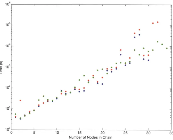
Naturally the simulation time went up as the number of nodes increased, see Figure 2-3 Simulation times could also be effected by the specific parameters, although nothing specific was noted. Sometimes certain sets of parameters would cause the

10 5 10 -4S 10-* S . 10 102 1 Os 100 -010 0 5 10 15 20 25 30 35

Number of Nodes in Chain

Figure 2-3: The time to simulate the BISH model as a function of number of nodes in the chain.

simulation to error out before it had completed. This created a great deal of difficulty when attempting to perform optimizations.

2-.5

Modes of Motion

Unsurprisingly the modes of motion for a chain are different than for a single node. For a single node to go in a helix, you need a force that creates a circular motion,

and then some propulsion component that twists the node along its

axis. This

additional component can either be a torque with a or the force is not applied to a point along the z axis. Table 2.1 lays this out in more detail.

Helical motion of the nodes in the chain was the predominant form of motion. In all simulations, the chain was started from an initial rest configuration with the

Table 2.1: Modes of motion and associated propulsion parameters for a single node

Case

Propulsion Position

Force

Torque

Motion

Conditions

A

[0,

0, -lz]

[0, 0, Fz]

[0,0,0]

straight

none

B

[0, 0 - lz]

[F, Fy, Fz]

[0,0,0]

Circle

Fx #0 or FY / 0

FX#0

or F #0

C

[l2,

Y, lz]

[Fx,

Fy, Fz) [0,0,0]

Helix

ix

0 or

1

_{y 4}

lX

0 or ly

f

0

D

[0, 0,lz

[Fx, Fy, F]

[0,0,-z]

Helix

Fx# 0 or Fy

#

0

chain in a line; all initial state values were zero. It turns out that a force applied not

pointing at the center of mass on a point off center seems to be all that is necessary

to get helical motion for a single node, case B in Table 2.1. A torque as a component

of the propulsion is not necessary. Figure 2-4 shows a sample helical motion after

transitory behavior.

Equation 2.4 gives expressions for the position and orientation of the center of

mass during helical motion along the z-axis.

x = r cos(kt)

y = r sin(kt)

z = vt

(2.4)

#

=

kt + $o

General expressions for the position and velocity of the center of mass moving in

a helix in an arbitrary direction are of the form:

x

xO

0

+

v

t

+ r sin(kt

+

o)()

x

=

vx +

rk cos(kt

+

$o)

and likewise for the y and z components. This is the equation that was fitted to the

results of the simulations in order to determine the parameters of the helix that was

present. The radius of the helix is r and the forward velocity v; their components are

given along world coordinates and designated by subscripts. The rotational velocity

50 40 30 20 10 0 -10 500 600

Time (s)

Figure 2-4: Example of center of mass motion during helical motion.

First Node

300 400 500 600 700 800 900 1000

time (s)

Middle Node

time (s)

Last Node

I I I I III-300 400 500 600 700 800 900 1000

time (s)

Figure 2-5: The x component of the center of mass velocities in the inertial frame of

a chain moving in a helix along a helical trajectory.

100 200 300 400 C 0 C,, 0

a- 0.2-0.1 - 00.1 - -0.2-200 0

E

0 0 CD 0.5 0 -0.5 '-200

of the helix is k; the final value was the average from the three fits. The value of r

was calculated from its components as follows:

r--VrX2 +

_r

rY2 +j rj2(26

_{= .(2.6)}

Other modes of motion were observed. One, referred to as a helical helix is where

the chain is swimming in a helical mode; however, instead of following a straight

line, such as in equations 2.4 and 2.5, it traces out a helical path. Figure 2-5 shows

position plots of the helical helix, which can be compared to Figure 2-4 which shows

a chain in its helical mode tracing out a straight line.

Other modes of motion were observed, but they generally had a helical component

except in the trivial case where everything just moved straight. In this thesis I

typically used a simpler set of parameters that what gives rise to the helical helix.

The important difference being the point the propulsion is applied to is off only in its

z component from the center of mass. The intuition for why the helical helix motion

arose is a result of the point where the propulsion was applied. When the propulsion

force was applied to the mass at a point away from the center of mass in both the 2

and

Q

directions, the

Q

component causes the propulsion force to cause a torque in the

z-direction about the center of mass on the node. This extra rotational component

creates the extra rotational component seen as the helical path the chain traces out.

Constraining the universal joints to

±900

and modeling the center of pressure

behind the center of mass, prevented the chain from moving erratically. In these

cases it was observed that the universal joint angles were both be near 180 degrees,

which is equivalent to the constrained rotational degree of freedom being rotated by

180 , which effectively causes the the x and y components of the propulsion to switch

direction for that particular node. Since a few nodes in the chain would then have

propulsion pointing in distinctly different direction erratic behavior would result.

2.6

Model Validation

The model was validated in a handful of ways. A single node simulation was performed using one node from the simMechanics model and another that was numerically in-tegrated from the derived equations of motion given in Appendix A. The equations for helical motion from the simulation of a single node, was numerically plugged into the equations derived for a single node, and this agreed for the center of mass motion and angular velocity, although the angular acceleration terms did not agree. This was assumed to be caused by an error on my part and not suggesting something wrong with the simMechanics model. Equation 2.5 was fit to results from the simMechanics simulation and R2 values were very high often at least 0.999 and sometimes 1.

In addition, identical simulations were run hundreds of times in a row, and the speeds after transients went away were compared. This was done three times with random selection of propulsion angles and the standard deviations of the speeds was on the order to 10-13. This is the same set of parameters used in the propulsion angle optimization. This showed that there are no numerical instabilities, nor any random or pseudorandom effects causing simulations to vary.

A qualitative validation of the conclusion that a chain will move with some kind

of helical motion when the propulsion is at an angle with respect to the z axis was done by building a ten node chain and observing it swimming in water with a few different sets of parameters. The chain swam in a helical mode of motion except when the rudders were set at 00; see chapter 5 for more details.

Chapter 3

Optimization

3.1

Introduction

One of the reasons for bio-mimicry and bio-inspiration in engineering is that nature often has highly optimized mechanisms for its environment. I was curious what kind of results would emerge if I optimized the chain for group speed, and searched over parameters such as propulsion angle, and the length and orientation of linkages between nodes. Due to a few issues discussed below, the only results obtained during the course of this research were for a specific case of optimizing the angle of the propulsive force.

3.2

Stochastic Gradient Search

To optimize the parameters of the robot, a stochastic gradient descent algorithm was employed: take a parameter vector a, a cost function to minimize J(a), and a learning rate 7. The algorithm approximates the gradient by running a simulation at a and at

#

+ a.

#

is a small random variable. The update is then given by[5]:

The algorithm works with each component of 0 drawn from a mean zero gaussian dis-tribution or when 0 is drawn from the shell disdis-tribution [5]. The shell distribution is where

3

is of constant magnitude and the direction is drawn from a uniform distribu-tion. Both distributions were used, but no differences were observed in the behavior of the algorithm, because other problems occurred, which overwhelmed whatever the effect of the different probability distributions.

This algorithm was used for a handful of reasons. It scales as the number of parameters being optimized, so even for a 20 link chain, which has 24 degrees-of-freedom, if it is optimizing four parameters, the search algorithm itself only operates in a four dimensional space. The simulation time of the system of course does increase as the number of nodes increases (Figure 2-3), so the actual optimization time can still be quite long for a chain with many nodes.

Most search algorithms require some means of calculating or approximating the gradient. Since to analytically calculate the gradients of a cost function like speed of a helix in terms of parameters of the chain seemed very difficult, it was desirable to have an algorithm that did not need the gradients handed to it.

/

had a standard deviation of 0.1 when drawn from a gaussian distribution, and had a magnitude of 0.1 or 0.01 when drawn from a shell distribution. The idea is to choose

/

large enough so the signal to noise ratio is high enough to get a good measure of the gradient, but small enough that it still provides a good local approximation of the gradient. q was often decreased by some small factor every iteration in order to help it to converge to the minimum closer. This factor was tried at several different levels. If q was kept constant at a smaller value it would have been easier to see the algorithm converging, but because simulation times of long chains are so long, it was desirable to try and speed up the algorithm by starting with a larger 7q. The other issue with shrinking q is the has the number of iterations grows 77 becomes so small that the cost is not going to noticeably decrease anymore regardless of whether or

3.3

Results

3.3.1

Propulsion Angle

The value function was the main traveling velocity of the helix. The speed was

chosen as the value function because Weelia cylindrica in its aggregate form is a fast

swimmer compared to other species [3]. The two optimization variables were the two

angles controlling the direction of the propulsion. The other parameters were chosen

to be reasonably close to those used when the chain was built and they are given in

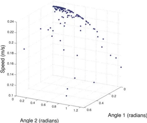
Appendix B. The points visited by the algorithm are shown in Figure 3-1. The final

result reached had propulsion angles of 0 and 0.0676 radians (3.8702 degrees), which

is nearly inline with the longitudinal (2) axis. The final velocity reached was 0.23

m/s. When both angles were set to 0, the speed was slightly slower by 0.00075 m/s.

I would have expected straight to be the fastest, but perhaps is has something to do

with the small torque (0.001 Nm) in the propulsion. The final speed reached is also

faster than typical speeds for Weelia cylindrica which are around 0.01 m/s to 0.1 m/s

[3][6][7].

This optimization was performed with 3 drawn from a mean zero gaussian

distri-bution. While it does appear the algorithm converged near the global maximum,

it jumped around quite a bit. The initial starting point was actually very near

the optimal [-0.2308, -0.2308],

although the algorithm visited points as far away

as [0.6069, 0.9382]. This was likely due to the large learning rate of the algorithm

initially, since the cost function appears smooth and convex in Figure 3-1.

3.3.2

Optimization issues and incomplete/failed attempts

In an effort to further support the optimum found in the preceding section, I ran

the algorithm 50 times from random initial angles, the results are shown in Figure

3-2. The plot shows that most of the time the algorithm did not complete the first

iteration; these points are the red, and have an arbitrary value of -0.666 assigned to

them. These failed attempts at optimization were due to some sets of parameters

0.24- 0.22-0.2

E

0.18 0.16 .) 0.14- 0.12-0.10. 0.4 0. 1.2 0.6 * 0 0. 0 %PNi 0g 9

Angle 2 (radians)

Figure 3-1: All points visited by stochastic gradient

propulsion angle.

* Got to final iteration

* Errored out Did not learn

0.6 0.2

E

0 -0.2 C) *4* -0.4 -0.64 ** * * **

Angle 1 (radians)

while searching for the optimal

* * * ~** # .**

*4*

* :* ~ 4 ~ ** 0 t * * 0.5

Angle 2 (radians)

Angle 1 (radians)

Figure 3-2: Results of 50 runs of propulsion angle optimization. Showing that many

times the simulations necessary halt due to errors. All the red dots at the bottom

halted on the first iterations of the optimization.

being significantly more difficult for the numerical simulation to handle. One of the other problems that happened only twice in this set of optimization, but was observed as a common problem, was the algorithm would get stuck in one small portion of parameters space, even though it did not appear to be a local minimum. Reasons for this are uncertain; it could be that some areas of parameter space are more numerically sensitive, perhaps making the cost function no longer smooth.

One of the differences between different species of salps is the architecture of their aggregate forms. I thought it would be interesting to see what would happen when the optimization was run over the parameters of the linkages between nodes, but no meaningful results were obtained, since this required searching over a larger number of parameters, which resulted in an even higher number of cases, where there were sets of parameters that could not be simulated.

A set of optimizations were also attempted to search over parameters of pulsed

propulsion, although in this case it was too difficult to know if the optimization converged in the set number of iterations, and even if any of the final points reached were local minimum, let alone a global minimum. This could probably be remedied

by better tuning of the optimization algorithm.

3.3.3

Conclusions and Suggestions for Improvements

A salp-like chain model was created in Matlab's SimMechanics toolbox, which

al-lowed investigation into the modes of motion such a chain as it swims. One partic-ular chain's propulsion angles were optimized for speed, creating a chain that moves nearly straight. Further optimizations could probably be successfully performed by improving the solver parameters, and creating a more robust optimization algorithm.

Chapter 4

Contraction and Stability Analysis

4.1

Introduction

Once the universal joints were limited in simulation to ±900 and some other details of the simulation were corrected, the chains for various sets of parameters always converged to a limit cycle, with some sort of helical nature to it. It was desired to try and determine whether the helical motion was an emergent behavior and, if so, under what relations between the parameters characterizing a simulated salp chain this would emerge. To this end, contraction analysis was attempted, since it provides certification that all trajectories of a system converge to the same trajectory, and it was hoped to show contraction to a helical trajectory. A set of simulations were performed to less rigorously provide insight into any emergent nature of the chains motion and see if there were any observable transition points, as with some contracting systems where, after a certain number of nodes are in the system, the emergent behavior changes and then persists.

4.2

Dynamic Equations

4.2.1

Variable Descriptions

State vector of a single node:

S =

Euler Angles:

0

[

=q>

Vector from the center of mass to the connection at its front to the i-1 node in coordinates fixed to the body:

XI

rf 0

ZI

Vector from the center of mass to the connection to the i+1 node in body coordi-nates: Xb rb= 0 -Zb (4.4) (4.3)

4.2.2

Equation for a Single Node

The equations of motion for a single node are given by rigid body dynamics [10].

Appendix A contains a fuller derivation.

A

=

f(s)

_(4.5)

x x 6) (4.1) (4.2)

k R(Fp+FD) = 1 _(4.6)

(I, - Iz)wywz

I-1(z

- Iz)Wz + -1(rp XFp +TT) (12: - I,)Wz,.

4.3

Initial Attempt at Contraction Analysis:

Cou-pling Terms

The ith node is connected at its front to the i-1 node and at its back to the i+1 node. rf being the vector from the universal joint to the center of mass, for the front connection, and rb being the vector from the center of mass to the joint that connects to the i+1 node. I originally tried to model the nodes as connected by an ideal universal joint, so a rigid connection except for two rotational degrees of freedom, causing the nodes to have a common

4.

However this results in the coupling terms not being simply a function of the state, s, but also 9. This would naturally create redundant equations, and prevent a model of the form:

si = f(s) + g(si-1, Si, Si+1)- (4.7)

where f(si) is the dynamics for the node and g(si_1j, si, si+1) represents all coupling terms between nodes. To get around this each of the rigid components of the con-nections was modeled as a spring with a very high spring constant. Torque from the spring on the rotational degree of freedom that is constrained by the universal joint:

0

r =0 (4.8)

. The torque induced by the force from the linear springs on the back and front of

the node, that replace the constant length linkage to the universal joint:

Tb = rb x [R[Ki(xi+1 - xi) + RTRi+lrb] (4.9)

rf = rf x [RTKI(xi - xi) + RT Ri-ir] (4.10)

No damping was modeled since that results from the water the BISH would swim in. This leads to the following coupling terms:

0

Li =K(xi_1 - 2xi

+

i+1

+

Rirb - Ri(rf + rb)

+R+r)

(4.11) Tr. ± Tb ± Tf

The form which these equations take prevents separating Li into g(si)

+

g(si_1)

+

g(si+1). This means techniques of simple virtual systems for coupled systems [2] cannot be used to perform contraction analysis. Coupling terms like RTRilrb mean Li is not affine in the state, so techniques from networks where the coupling can be written in the form Lx [2} are also unavailable for analysis of the BISH.

4.4

Contraction Analysis: The Jacobian

Because the desired behavior is locomotion in a limit cycle, the contraction of x or

0, is not only irrelevant, but these dynamics are unstable, because I want indefinite locomotion of the helix, so those dynamics will be ignored. A new system with the state only composed of * and w leads to

yi = g(yj) + L(yi, yi-1, yi+1) (4.12)

Furthermore, because of the issues stated above, the Jacobian of the entire system must be considered. If it is shown to be negative definite under some coordinate

transform 0. Concatenating the dynamic systems for all the nodes together leads to:

(4.13)

The next step is to form the generalized Jacobian:

(4.14)

F = 0--G ~1 + W0~,

_F=8r1±O

This can be thought of as taking the Jacobian after a coordinate transformation.

RT 0

When 0 is block diagonal with blocks , this corresponds to forming the

0 I

Jacobian by taking derivatives with respect to velocities in the frame fixed to each node, since the velocities in y1 in 4.13 are in the world frame. Note that L does

not depend on x or w, so it has no contribution to the Jacobian, so 0-20-1 is block diagonal. Each block is the Jacobian of the respective individual node. The remaining term of the generalized Jacobian,

F

is given by:

g-1

= 0 Wz -WY 0 0 0

WZ

0 0x 0 0 0 WY 0 0 0 0 0 0 0 0 0 0 0 0 0 0 0 0 0 0 0

0

0 0 (4.15)

The symmetric part of this matrix is 0, so it doesn't contribute anything to the evaluation of the negative definiteness of F. So for the purposes of this analysis F is now block diagonal composed of n of the following matrices, each only containing

state variables of a single node.

-2c.|k|

0 0 0 0 0

0

-2c.,|Q| 0 0 0 0

0

0

-2czIi|

0

0

0

0

-2rc&PcVWi/I2

0

-2bx Jwx|/12x (Iy - Iz)LLz/I, (ly - Iz)Lvy/I,

2rc,,c2|Il/I, 0 0 (Iz - Ix)bwz/Iy -2by|wy|/I, (Iz - Ix)wx/I,

0 0 0 (Ix - I)w/Iz (Ix - Iy)w2/I2 -2bzlwzl/Iz

(4.16)

Since all the blocks are identical, it is only necessary to examine one of them to determine if F is negative definite. The upper left corner is clearly negative definite. The lower right corner however poses a problem. While it can be simplified due to cylindrical symmetry (I2 =

I,),

I was unable to derive a result that was independent of extra information about w. Sticking constants together and taking the symmetric part of the bottom right 3x3 matrix yields:

-2bi w2|

0

b2Wy/2

0

-2bily|

-bwx/2

(4.17)

b2wy/2 -bw2/2 -2b 3

|w.2-The determinates of the upper 1xi and 2x2 matrices are negative and positive as required for negative definiteness, however the determinate of the whole matrix yields the following condition:

bib2IwI 3

₊

_{bib |w1Y}3

_<

_4b

_b

3w2TIWYIIlz (4.18)

This clearly will not always be true without some guarantees on the relationships between the angular velocities. The z-axis has the largest moment of inertia, so wz would tend to dominate without the presence of external forces, but since it is under a constant propulsion force, this is clearly not the case and more work is needed to achieve an insightful analysis of this system. Failing the ability to show the BISH to be a contracting system, it was still desired to see if there were emergent properties

of the systems behavior.

4.5

Emergent Behavior

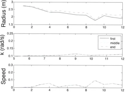
A set of simulations was run on chains from one to twelve nodes in length, to see how

the size and speed of the helical swimming mode changed with length (Figure 4-1).

See Appendix B for the precise parameters used for these simulations.

The speed and angular velocity for the first, middle, and end nodes are all the

same for all chain lengths. This means the chains are not bunching up or twisting

into a tighter helix. This supports that the helix fitted is a limited cycle. All R

2

values for the fits were nearly at least 0.9999. One thing worth noting is that the

chain did seem to have a larger radius towards the back.

The general trend is higher smaller radius, slightly higher spin (the angular

ve-locity of the helical motion), and generally increasing speed. The rough correlation

between these values makes sense, because the smaller the radius, likely the more the

propulsion is pointing forward, so the higher the speed.

A single node swims in a circle with a speed of 0.232 m/s (the helix speed was 0).

The largest speed for a chain was 0.097 m/s with a length of nine nodes. This does

not show anything analogous to Weelia cylindrica, whose aggregate speed can exceed

0.1 m/s, but whose solitary speed is 0.06 m/s [3]. This is probably due to the model

of hydrodynamic drag used, which does not account for any drafting between nodes

or streamlining.

No threshold on the behavior as a function of chain length was observed. If this

had occurred, it would be consistent with the hope of a tractable contraction

anal-ysis, since contraction analysis is used to show such effects in networks and coupled

oscillators.

E 3

E

25-Co. -2-1.5 0 2 4 6 8 10 12 0.25 0.2 - first middle C . _end 0.15-0.1 --- I - -5 6 7 8 9 10 11 12 0.3 S0.2-C- 0.1 -0,: - -- -~ 0 2 4 6 8 10 12

Figure 4-1: Parameters of helical motion as a function of number of nodes in the

chain.

Chapter 5

Physical Implementation

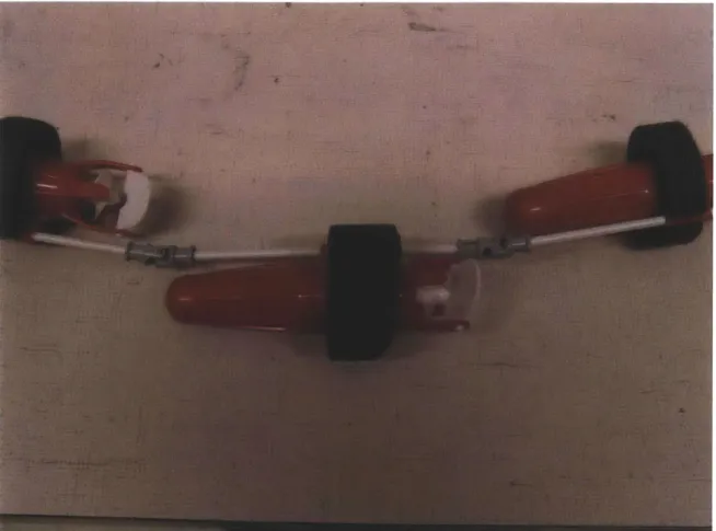
A robot was built to demonstrate some of the basic concepts found in the simulations.

It confirmed that the presence of a torque and off-axis force can make a helical

swim-ming motion. A ten node chain that formed a helix as it swam was demonstrated. The

chain was constructed from ten independent propeller modules. The unit used was

a Tamiya Submarine Motor, Mini High-Speed Type (Tamiya Item Number 70185).

This is a self contained unit with a AAA battery motor and propeller. The units

were connected with pieces of 1/8 in. fiberglass rod and LEGOTM universal joints.

Sealed cell pipe insulation foam was attached to each node to make it near neutrally

buoyant. The connections between the fiberglass rod and each unit were left free

to rotate so the chain could be tried in different configurations. Figure 5-2 shows a

typical configuration of the chain of nodes and Figure 5-1 shows a close up.

A few experiments were also done with a single node, verifying that with the

rudder at an angle the node would move in a helix. This verifies the torque and force

produced by the propeller is enough to make a single node move in a helix, which

was also demonstrated in simulation.

The primary distinction between this chain and what was often used in simulation

is that the propeller produces both a force and a torque, while the vortex ring from

a salp produces only a force. Most of the simulations were done with only a force,

although some were performed with a torque. The simulations also did not model

gravity or buoyancy, which is the equivalent to each node being neutrally buoyant

Figure 5-1: A single node of the BISH and its neighbors

and the center of mass at the same location as the center of buoyancy.

The rudders were adjustable and experiments were performed at a few different

angles. The only result the experiments clearly demonstrated was that when all the

rudders are straight

(00

with respect to the long axis of each node), the chain does

not form into a helix, but with the rudders at an angle (a few angles in the range of

30' to 90' were tried), a helix does indeed form. Figure 5-3 shows frames from about

every half second of one such experiment.

The third rotational degree of freedom was not completely fixed, because it was

just friction fitted, and in many cases some nodes orientations changed. This was not

a huge concern, since the experimental setup did not allow for much measurement of

the actual size or speed of the helix.

Buoyancy effects prevented the chain from swimming in anything but a

predomi-nantly vertical direction, which prevented observations of more then a few rotations

of the helix. The chain was constructed to be near neutrally buoyant. In practice this

cannot be achieved perfectly; this, combined with the center of buoyancy not being

at the same location as the center of mass, made it impossible to get the chain to

move in a primarily horizontal direction. Most tests ended up being performed with

the chain not quite neutrally buoyant, so it would slowly sink, face the bottom, and

then swim toward the bottom. Since the chain was 1.11 meters (43.75 inches) long,

and the pool only 3.96 meters (13 feet) deep this only allowed observations of at most

two or three rotations of the helix before it hit the bottom of the pool. The final

frame in figure 5-3 shows when the lowest node has just touched or is about to touch

the bottom of the pool.

Chapter 6

Conclusion and Suggestions for

Future Work

The basis for the helical motion is the result of an off axis force, which creates both a spinning and a translational motion, causing a helix. In the contraction analysis I was unable to show the Jacobian to be negative definite due to the condition in equation 4.18. However the system does still appear to display emergent behavior at times, forming helixes that trace out straight paths or helical paths. The basic helical mode of motion and the BISH's contraction towards such a trajectory were demonstrated

qualitatively by the construction of a ten node chain.

There are many possibilities for future analysis of BISH. While I was unable to get results from the contraction analysis, it is possible a chain with a different morphology could yield a successful analysis, or more advanced mathematics. It could also be worth deriving conditions under which the helical mode is a solution to the equations of motion, and not the helical helix, or other modes of motion.

Using Langrangian dynamics the full equations of motion for a chain could be written out. There may be some insights to be gained by examining the equations of motion. It may be possible to write out analytic gradients, which would allow other optimizations algorithms to be used.

The optimizations attempted in this thesis could probably be made to work better,

in the successful simulations more often. Simulating a shorter chain, would result in the algorithm running faster. Parameters more precisely modeling real salps could be used. A drag model that includes drafting would be useful for future investigations into the morphology of the aggregates.

In terms of hydrodynamic drag the most efficient I hypothesize is probably when spiraling and moving forward such that other than skin drag the only drag is on the front, it's precisely following along in the spiral. Everything else would require pushing more water aside. This could be used as the assumed motion and than perform analysis on a chain that acts that way.

There is room for a lot more research in similar swimming chains. Not investigated at all in this thesis are questions of how to construct a robot of this structure that can swim around freely, it would be an interesting test bed for distributed and under-actuated control. The efficiencies of a distributed propulsion present in chains like this, is also an area worth investigating, since like many other areas in engineering, nature has a lot to teach us about efficiency.

Appendix A

Derivation of Equations for Single

Node

This appendix contains a derivation of the equations of motion for a single node of a BISH. It is a single rigid body with forces and torques acting on it in 3D space. The body fixed axis is that shown in 2-1.

A.1

Variable Descriptions

Euler angles were used to describe the rotation of each node.

0

05

(A.1)

The z-y-x convention was used, meaning to go from the world coordinate reference frame first rotate

4

about the z axis, then V) about the resulting intermediate y-axis then 0 about the resulting x-axis, which is the body-fixed coordinate frame x-axis. Transforming a vector from global coordinates to local coordinates then takes the form:

Sign conventions must be observed, since opposite signs are used for the angles when converting vectors as compared to rotating reference frames, or equivalently different rotation matrices.

The state vector is composed of positions,x, and velocities,*, with respect to inertial world coordinates frame; euler angles as described above; and angular velocity

w with components along the body fixed axes.

x k

s = (A.3)

0

Moment of Inertia in the body frame:

I2 0 0

1= 0 IV 0 (A.4)

0O 0 IzJ

In all cases considered in this thesis Ix = I, and Iz > Ix.

The center of pressure is the point on the body where all drag forces and torques are applied. This is represented as a vector from the center of mass to the center of pressure in body coordinates:

0

rc

[=

0 (A.5)

-rco,

This rotation matrix rotates from a set of body fixed axis to the global frame:

cos(4) cos(#) - cos(0) sin(0) sin(4) cos(#b) sin(#) + cos(O) sin(V)) cos(#) sin(4@) sin(O)

R = - cos(#) sin(V)) - cos(9) cos(V)) sin(#) cos(O) cos(7p) cos(#) - sin(#) sin(#) cos(V)) sin(O)

sin(#) sin(9) - cos(#) sin(9) cos(O)

(A.6)

angles to angular velocities. cos(#) T = E sin(O) _ sin(#) tan(O)

-

_{sin(#) 0}

cos(#) ₀ sin(O) cos(#) tan(O) _

Translational drag equation given with velocities in the local frame:

FDiocal =

-cIi

Pii

CyAi I I

czii

I

zi|

Translational drag equation given with velocities in the global frame:

cFj 0

0

FD -0 Cy 0 0 0 czj

|RTdiag(k)|R

I

(A.9)

Rotational drag equation in the local frame:

b2wxIWXI1

TD = - bywyw (A.10)

bzwz Iwz

I

Total of all drag terms that canse a torque on the node. This variable is used for notational simplicity:

TT = rCOP x FD + TD (A.11)

The equations of motion for a single node are given by rigid body dynamics [10].

A

= f (s)

(A.12)

(A.7)

x R(F,

+

FD)

T-'w

( I V - I z ) w y wz _{- r}

_~

T

I-i

(I. - I.)wzw +I1(rxF,+T)

Appendix B

Paramters for BISH simulations

B.1

_{Parameters for Propulsion Angle}

Optimiza-tion

This appendix contains sets of parameters used for the BISH simulations.

_{'salp' in}

the comments in the code is used to refer to a node in the simulation, not necessarily

a real salp.

These are the parameters used for the simulations for the propulsion angle

opti-mization in section 3.3.1.

1 %All the parameters for the salp simulation

2 %all units are assumed to be degrees and mks 3 clear all;

4 close all;

5 _{global uAmplitudeEven xFinal valueHist alphaHist oddTorque evenTorque} 6

8 %general parameters

9 sLength = 0.14; %the length of a salp

10 sRadius = 0.02; %the radius of the salp.

11

13 0

14 %Parameters for the salp body

15 %

16 %all frames of a single body are assumed to be aligned with CS1 ...

(the front

17 %connection), which is then rotated with respect to the adjoining frame

18 %(the back connection of the previous salp).

19 %z points in the direction of forward travel. x is the "left-right" 20 %direction where salps are to the left and right of each other. 21 %==

22 % CURRENTLY ARBITRARY!

23 sMass = 0.04; %about 40 grams %Mass of the salp 24

25 % CURRENTLY ARBITRARY!

26 sInertia = [.0008 0 0; 0 .0008 0; 0 0 .0004]; %moment of inertia .. tensor of the salp.

27

28

29 %CS1->CG

30 %vector pointing from the forward connection point (CS1) to the ... center of

31 %gravity (CG) in components of the body coordinate frame.

32 frontConnect = [0 -sRadius*l -sLength];

33

34 %CG->CS2

35 %vector pointing from the center fo gravity (CG) to the back ... connection

36 %point (CS2) in components of the body coordinate frames.

37 backConnect = [0 sRadius*l -sLength]; 38

39 %CG->CS3

40 %the vector from the center of gravity to where the propulsion ... acts (CS3)

41 propulsionPosition = [0 0 -sLength]; %[0 sRadius*0.5 -sLength*0.5]; 42

43 %CS2 -prev->CSl current

44 %orientation vector of Euler angles (x y z) of one salp with ...

respect to the

45 %previous salp. Orientation of CS1 to adjoining. 46 connectR = [0 0 30];

47 %can use this to set the initial orientation fo the salp, when ...

there's only

48 %one.

49

50 relRotInit = [0 0]; %the initial angles of the universal joint ...

between salps

51

52 %Params for limiting the motion of the universal joint

53 angleLimit = 90; %needs to be in same units as angle sensor (degrees)

54 angleConstraintK = 400; %spring constant,

55 angleConstraintB = 25; %damping constant. a little over damped

56

57 %Center of pressure position

58 COPPosition = [0 0 -sLength];

59

60 %spring constant for springs joining a small mass that has the ...

drag force

61 %applied to it to the main salp body.

62 kDrag = [360 360 360 100 100 100]*100*sMass;

63

64 %damping coefficients for same springs to get critically damped ...

system 65 bDrag = 2*sqrt(kDrag*1.01*sMass); 66 %[360 360 360 10 10 10]*10; 67 68 69 %%========================================= 70 rho-water = le3; 71

72 %10times should only be temporary