HAL Id: hal-02902728
https://hal.archives-ouvertes.fr/hal-02902728
Submitted on 28 Aug 2020
HAL is a multi-disciplinary open access
archive for the deposit and dissemination of
sci-entific research documents, whether they are
pub-lished or not. The documents may come from
teaching and research institutions in France or
abroad, or from public or private research centers.
L’archive ouverte pluridisciplinaire HAL, est
destinée au dépôt et à la diffusion de documents
scientifiques de niveau recherche, publiés ou non,
émanant des établissements d’enseignement et de
recherche français ou étrangers, des laboratoires
publics ou privés.
Distributed under a Creative Commons Attribution| 4.0 International License
International challenge to model the long-range
transport of radioxenon released from medical isotope
production to six Comprehensive Nuclear-Test-Ban
Treaty monitoring stations
Christian Maurer, Jonathan Baré, Jolanta Kusmierczyk-Michulec, Alice
Crawford, Paul Eslinger, Petra Seibert, Blake Orr, Anne Philipp, Ole Ross,
Sylvia Generoso, et al.
To cite this version:
Christian Maurer, Jonathan Baré, Jolanta Kusmierczyk-Michulec, Alice Crawford, Paul Eslinger, et
al.. International challenge to model the long-range transport of radioxenon released from medical
isotope production to six Comprehensive Nuclear-Test-Ban Treaty monitoring stations. Journal of
Environmental Radioactivity, Elsevier, 2018, 192, pp.667-686. �10.1016/j.jenvrad.2018.01.030�.
�hal-02902728�
Contents lists available atScienceDirect
Journal of Environmental Radioactivity
journal homepage:www.elsevier.com/locate/jenvrad
International challenge to model the long-range transport of radioxenon
released from medical isotope production to six Comprehensive
Nuclear-Test-Ban Treaty monitoring stations
Christian Maurer
a,∗, Jonathan Baré
b, Jolanta Kusmierczyk-Michulec
b, Alice Crawford
c,
Paul W. Eslinger
d, Petra Seibert
e, Blake Orr
f, Anne Philipp
g, Ole Ross
h, Sylvia Generoso
i,
Pascal Achim
i, Michael Schoeppner
b,j, Alain Malo
k, Anders Ringbom
l, Olivier Saunier
m,
Denis Quèlo
m, Anne Mathieu
m, Yuichi Kijima
n, Ariel Stein
c, Tianfeng Chai
c, Fong Ngan
c,
Susan J. Leadbetter
o, Pieter De Meutter
p, Andy Delcloo
p, Rich Britton
q, Ashley Davies
q,
Lee G. Glascoe
r, Donald D. Lucas
r, Matthew D. Simpson
r, Phil Vogt
r, Martin Kalinowski
b,
Theodore W. Bowyer
daZentralanstalt fuer Meteorologie und Geodynamik (ZAMG), Hohe Warte 38, 1190 Vienna, Austria bComprehensive Nuclear-Test-Ban Treaty Organization, International Data Center, Vienna, Austria cNational Oceanic and Atmospheric Administration Air Resources Laboratory, College Park, MD, USA dPacific Northwest National Laboratory, Richland, WA, USA
eUniversity of Natural Resources and Life Sciences, Institute of Meteorology, Vienna, Austria fAustralian Radiation Protection and Nuclear Safety Agency, Yallambie, Miranda, Australia gUniversity of Vienna, Department of Meteorology and Geophysics, Vienna, Austria hFederal Institute for Geosciences and Natural Resources (BGR), Hannover, Germany iCommissariat à l’Énergie Atomique, Arpajon, France
jPrinceton University, Program on Science and Global Security, Princeton, NJ, USA
kEnvironment and Climate Change Canada, Meteorological Service of Canada, Canadian Meteorological Centre, Environmental Emergency Response Section, RSMC
Montreal, Dorval, Québec, Canada
lSwedish Defence Research Agency, Stockholm, Sweden
mFrench Institute for Radiation Protection and Nuclear Safety, Fontenay-aux-Roses, France nJapan Atomic Energy Agency, Tokai, Ibaraki, Japan
oMet. Office, Exeter, Devon, UK
pBelgian Nuclear Research Center, Mol, Belgium & Royal Meteorological Institute of Belgium, Brussels, Belgium qUnited Kingdom-National Data Center (NDC), Aldermaston, Reading, United Kingdom
rNational Atmospheric Release Advisory Center (NARAC) at the Lawrence Livermore National Laboratory (LLNL), Livermore, CA, USA
A R T I C L E I N F O
Keywords:Atmospheric transport modelling Nuclear explosion monitoring Medical isotope production Radioxenon background
Model inter-comparison and evaluation
A B S T R A C T
After performing afirst multi-model exercise in 2015 a comprehensive and technically more demanding at-mospheric transport modelling challenge was organized in 2016. Release data were provided by the Australian Nuclear Science and Technology Organization radiopharmaceutical facility in Sydney (Australia) for a one month period. Measured samples for the same time frame were gathered from six International Monitoring System stations in the Southern Hemisphere with distances to the source ranging between 680 (Melbourne) and about 17,000 km (Tristan da Cunha). Participants were prompted to work with unit emissions in pre-defined emission intervals (daily, half-daily, 3-hourly and hourly emission segment lengths) and in order to perform a blind test actual emission values were not provided to them. Despite the quite different settings of the two atmospheric transport modelling challenges there is common evidence that for long-range atmospheric transport using temporally highly resolved emissions and highly space-resolved meteorological inputfields has no sig-nificant advantage compared to using lower resolved ones. As well an uncertainty of up to 20% in the daily stack emission data turns out to be acceptable for the purpose of a study like this. Model performance at individual stations is quite diverse depending largely on successfully capturing boundary layer processes. No single model-meteorology combination performs best for all stations. Moreover, the stations statistics do not depend on the distance between the source and the individual stations. Finally, it became more evident how future exercises
https://doi.org/10.1016/j.jenvrad.2018.01.030
Received 24 August 2017; Received in revised form 31 January 2018; Accepted 31 January 2018
∗Corresponding author.
E-mail address:christian.maurer@zamg.ac.at(C. Maurer).
Available online 08 March 2018
0265-931X/ © 2018 The Authors. Published by Elsevier Ltd. This is an open access article under the CC BY-NC-ND license (http://creativecommons.org/licenses/BY-NC-ND/4.0/).
need to be designed. Set-up parameters like the meteorological driver or the output grid resolution should be pre-scribed in order to enhance diversity as well as comparability among model runs.
1. Introduction
The Comprehensive Nuclear-Test-Ban Treaty (CTBT), an interna-tional agreement to ban all nuclear tests, has developed a global net-work of 321 monitoring stations and 16 laboratories for verification purposes (CTBT, 1996), the International Monitoring System (IMS). It monitors seismic, hydroacoustic, infrasound and radionuclide sig-natures (CTBTO, 2017).
The radionuclide component comprises measurements of aerosol-bound radioactivity at 80 locations. Half of the 80 stations shall have additional equipment to measure ambient air concentrations of four radioactive xenon isotopes (Xe-131 m, Xe-133, Xe-133 m, and Xe-135) produced in nuclear explosions. 31 noble gas stations are already in operation, and 25 of those have been certified by the Comprehensive Nuclear-Test-Ban Treaty Organization (CTBTO).
In 1999, the International Noble Gas Experiment (INGE) was laun-ched to determine the feasibility of building and deploying automated systems to detect the four radioactive xenon (radioxenon) isotopes of interest (Auer et al., 2010; Bowyer et al., 2002). Commercial versions of three of the four radioxenon detection systems developed for the INGE are now deployed in the IMS: 1) The Automatic Radioanalyzer for Isotopic Xenon (ARIX), from the Khlopin Radium Institute, Russia (Dubasov et al., 2005), 2) the Swedish Automatic Unit for Noble Gas Acquisition (SAUNA, nowadays produced by Scienta Sauna Systems AB, Uppsala, Sweden), from Totalförsvarets Forskningsinstitut (FOI), Sweden (Ringbom et al., 2003), and 3) the Système de Prélèvement d' Air Automatique en Ligne avec l' Analyse radioXénons atmosphériques (SPALAX) from Departement Analyse, Surveillance, Environnement du Commissariat à l’Énergie Atomique (CEA/DASE), France (Fontaine et al., 2004).
Discrimination between radioxenon releases originating from a nuclear explosion or from civil facilities is a challenging task for the CTBTO. To our knowledge currently at least nine facilities worldwide are in operation: IRE located in Fleurus/Belgium, Mallinckrodt in Petten/the Netherlands, NIIAR in Dimitrovgrad/Russia, BaTek in Jakarta/Indonesia, NECSA in Pelindaba/South Africa, CENA in Ezeiza/ Argentina, HFETR in Chengdu/China, PINSTECH PAAR-1 in Islamabad/Pakistan and ANSTO in Lucas Heights/Australia (Gueibe et al., 2017; Achim et al., 2016). Atmospheric transport modelling (ATM) combined with isotopic ratio analysis (Kalinowski et al., 2010) can be considered as the most important means for achieving this goal. A large number of studies of the release and transport of radioxenon from nuclear power plants and medical isotope production and other man-made radionuclide emission facilities have been conducted to develop an understanding of background levels (Eslinger et al., 2014; Hoffman et al., 2009; Kalinowski et al., 2008; Saey et al., 2010; Wotawa et al., 2010, 2003; Zaehringer et al., 2009; Achim et al., 2016; Schoeppner, 2017). These studies confirm that fission-based production of molybdenum-99 for medical purposes is the largest routine con-tributor of radioxenon (which comes as a by-product of the production process) in the atmosphere, and that related releases can be detected at large distances. The Mo-99 daughter Tc-99 m is widely used for medical purposes (Peykov and Cameron (2014), approximately 30–40 million medical procedures per year) and a future growth in demand is ex-pected.
Radioxenon levels at IMS noble gas stations resulting from under-ground nuclear tests can be comparable to backunder-ground levels (Ringbom et al., 2014; Saey, 2009) and are thus harder to detect in regions under the influence from medical isotope production facilities. A reduction of their radioxenon releases would therefore be useful (Bowyer et al.,
2013). Nevertheless, medical isotope production facilities do meet regulatory release limits (Tinker et al., 2010; Hoffmann et al., 2001), thus their operators have little incentive for spending money on re-duction measures.
Although atmospheric modelling studies using inert tracers have been conducted since the early 1980s (e.g., Ferber et al., 1986; Gudiksen et al., 1984), detailed source-term data for the simulation of the transport of radioxenon from medical isotope production facilities have not been made available until recently. A 2013 study examined the regional impact of source-term data of different time resolutions on the capability to predict IMS radioxenon detections (Schoeppner et al., 2013). The study utilized emission data down to daily time resolution from the ANSTO facility close to Sydney (Australia) and detections in Australia and New Zealand. It found increasing agreement between simulations and detections from annual down to daily time resolution of the emission data. Little influences from other sources in the Southern Hemisphere were observed. A recent international model comparison (1st ATM Challenge,Eslinger et al. (2016)) used Xe-133 stack emission data from the Institut des Radioéléments (IRE) radio-pharmaceutical plant in Fleurus (Belgium) and activity concentration data collected at the IMS noble gas sampler at radionuclide station DEX33 (Schauinsland, Germany). The purpose of that exercise was to ascertain the level of agreement that can be achieved between Atmo-spheric Transport Models (ATMs) using stack monitoring data and xenon isotopic concentration measurements at IMS stations. One of the conclusions from that exercise was that using stack monitoring data to calculate radionuclide concentrations at a distance of about 400 km can match larger individual simulated sample concentrations (i.e., above 3 mBq m−3) to within±40% of the measured concentrations if an op-timally selected (according to the mean square error) ensemble mean of ATMs is used, and in some cases even lower deviations are achievable. Also, models using source term data in 15 min to 3 h time intervals produced similar agreement with measured concentrations as models using source term data averaged over longer intervals. In addition, even though the releases from IRE dominated the measured concentrations at DEX33, releases from other facilities such as nuclear power plants also influenced the smaller measured concentrations (see also De Meutter et al. (2016)). One of the benefits of that exercise was that it sparked many discussions on which techniques were most suitable, what knowledge and technique gaps exist, and what datafidelity is needed from stack monitors.
This current study also addresses the question of the level of agreement that can be achieved between IMS measurements and those simulated using Xe-133 stack release data and atmospheric transport modelling. Since ATM is a cornerstone of Treaty verification (Becker et al. (2007); Wotawa et al. (2003), including the discrimination be-tween military and civil radionuclide sources) the scenario team of the challenge (made up by ZAMG, CTBTO/IDC and PNNL) sought broad participation of the respective community. The role of ATM in Treaty verification should be underpinned. Having at hand a multitude of si-mulations an ensemble approach pays off since this is the only way of overcoming individual ATMs' deficiencies and uncertainties and re-producing related measured samples more accurately. Rere-producing measured radioxenon samples related to industrial production could be of great benefit to National Data Centers (NDCs,CTBT (1996)) which for verification purposes have to deal every month with a multitude of elevated radioxenon concentrations detected at IMS stations.
The setting of the current challenge is different in several ways compared to the previous one. Concentration data are used from six IMS radionuclide stations rather than just from one, as was used earlier.
The distance between the release point in Australia (ANSTO) and the samplers is between 680 and 17,000 km rather than 380 km. The new challenge is set in the Southern Hemisphere which has different weather circulation patterns than the Northern Hemisphere. In addi-tion, only the Koeberg complex in South Africa, the Atucha and Embalse complexes in Argentina and the Angra complex in Brazil have operating nuclear power plants, although releases from other medical isotope production facilities (e.g., Pelindaba in South Africa) can sometimes influence the selected IMS samplers (Eslinger et al., 2014). Overall radioxenon levels are lower in the Southern compared to the Northern Hemisphere (Achim et al., 2016). Just because of these dif-ferences between the two challenges it will be interesting to compare the two exercises in terms of qualitative, but also quantitative outcomes in order to deduce common characteristics.
2. Materials and methods 2.1. Participating organizations
Seventeen organizations from ten countries (Australia, Austria, Germany, France, Canada, Sweden, Japan, USA, United Kingdom and Belgium) took part in the 2nd ATM Challenge (Table 1). An overview of the models used is provided inTable 2together with some key para-meters of the model set-ups. Participants were encouraged to submit multiple runs, but were asked to submit at least one run using source term data with daily resolution, as radiopharmaceutical producers would– if at all – probably supply data with this resolution. There were up to six contributions per organization. Participants applied different model set-ups, different meteorological drivers in different spatial and/ or temporal resolutions and different spatial output resolutions. In total 97 simulations were performed, of which 30 were based on daily emission source resolution.
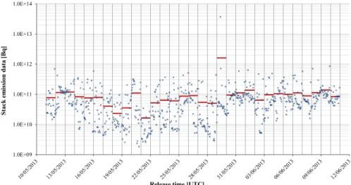
2.2. Stack emission data
The scenario team of the ATM Challenge received Xe-133 stack emission data from the Australian Nuclear Science and Technology Organization (ANSTO) radiopharmaceutical facility in Lucas Heights, Sydney, Australia (150.98° E and 34.05° S; see Fig. 2). The emission data cover a period of a month, from May, 11th, to June 10th, 2013. This period was chosen due to emission data availability, but also be-cause some stations had outstanding recordings of radioxenon during this period. Emissions at the stack were measured with a sodium-iodide (NaI) system based on the 81.0 keV gamma emission line of Xe-133. The activities were provided for 744 contiguous 1 h release periods, each one being the sum of four 900 s measurements, and are shown together with the daily average of hourly emissions inFig. 1.
During the period of interest for this ATM Challenge, it is observed that standard release quantities varied by as much as two orders of magnitude. The minimum activity measured by the system during this period is 1.83× 10⁹Bq (May 20th, 2013), the maximum activity is 3.67× 10¹³Bq (exceptional release on May 29th, 2013) and the median activity adds up to 5.46× 10¹⁰Bq. From one hour to the next, the typical variation of release quantities is by one order of magnitude, but var-iations by as much as two orders of magnitude are also observed from time to time.
In 2013 there were several process steps which could explain the variability of the releases. One of the main sources of peak emissions was the vacuum buffer tank. Solutions were moved around using va-cuum lines and if extra vava-cuum capacity was required during a pro-duction run, any off-gases it may have contained were released. A second source of peaked emissions was the regeneration of the hy-drogen convertor. Separately, whilst the facility was equipped with multiple gas storage tanks for trapping the off-gases from target dis-solution, there were no large banks of carbon to delay and smooth out any in-cell releases. The decay tanks were released after around seven weeks delay, giving rise to small emissions. Between production runs, maintenance and waste transfer activities were also associated with
Table 1
Participants of the 2nd ATM Challenge. Organizations participating in the 1st Challenge are printedbold.∗No blind test, involved in drafting the challenge. Organization
Abbreviation
Name(s) of participant(s) Organization full name Submission(s)
ARPANSA Blake Orr Australian Radiation Protection and Nuclear Safety Agency, Yallambie/Miranda,
Australia
ARPANSA
BGR Ole Ross Federal Institute for Geosciences and Natural Resources (BGR), Hannover, Germany BGR
BOKU Petra Seibert & Anne Philipp University of Natural Resources and Life Sciences, Institute of Meteorology & University of Vienna, Department of Meteorology and Geophysics; Vienna, Austria
BOKU1–6
CEA Sylvia Generoso & Pascal Achim Commissariat à l’Énergie Atomique, Arpajon, France CEA1–2
CTBTO* Jolanta Kusmierczyk-Michulec Comprehensive Nuclear-Test-Ban Treaty Organization, International Data Center, Vienna,
Austria
CTBTO1
CTBTO Michael Schoeppner Comprehensive Nuclear-Test-Ban Treaty Organization, International Data Center, Vienna, Austria
CTBTO2
ECCC-CMC Alain Malo Environment and Climate Change Canada, Meteorological Service of Canada, Canadian
Meteorological Center, Environmental Emergency Response Section, RSMC Montreal, Dorval, Québec, Canada
CMC1–2
FOI Anders Ringbom Swedish Defence Research Agency, Stockholm, Sweden FOI
IRSN Olivier Saunier, Denis Quèlo,
Anne Mathieu
French Institute for Radiation protection and Nuclear Safety, Fontenay-aux-Roses, France IRSN
JAEA Yuichi Kijima Japan Atomic Energy Agency, Tokai, Ibaraki, Japan JAEA
LLNL Lee G. Glascoe, Donald D. Lucas,
Matthew D. Simpson, Phil Vogt
National Atmospheric Release Advisory Center (NARAC) at the Lawrence Livermore National Laboratory (LLNL), Livermore, California, USA
LLNL1–2
Met. Office Susan J. Leadbetter Met. Office, Exeter, Devon, UK METOFFICE
NOAA-ARL Alice Crawford, Ariel Stein, Tianfeng Chai, Fong Ngan
National Oceanic and Atmospheric Administration Air Resources Laboratory, College Park, Maryland, USA
NOAA-ARL1–4
PNNL Paul W. Eslinger Pacific Northwest National Laboratory, Richland, Washington, USA PNNL
PU Michael Schoeppner Princeton University, Program on Science and Global Security, Princeton, New Jersey, USA
PU SCK•CEN RMI Pieter De Meutter & Andy Delcloo Belgian Nuclear Research Center, Mol, Belgium & Royal Meteorological Institute of
Belgium, Brussels, Belgium
SCKCEN RMI1–2
UK-NDC Rich Britton & Ashley Davies United Kingdom-National Data Center (NDC), Aldermaston, Reading, UK UK-NDC
Table 2 Models and set-ups used. Columns indicate the ID of the submission, the name of the atmospheric transport model (ATM), the meteorological model provi ding the meteorological input (NWP model), the horizontal, vertical (with number of model levels below 2.5 km including the surface level) and temporal resolution of the meteorological input (Meteorological input resolution), the horizo ntal output resolution, the top height(s) of the ATM output layer(s) above surface used for concentration averaging and temporal output resolution (Output resolution), the ATM simulation direction (Simulation direction, forward in time from the source/FWD or backward in time from a receptor/BWD), emission segment resolutions considered (Emission resolution) and the number of particles released per hour (#particles/hour released, k = 1000, M = 1 million). If not indicated v ia superscripts otherwise particle ranges refer to the particles used for low and high emission resolution runs. For the BOKU submissions the di ff erence is only in the horizontal and vertical averaging of dispersion output around the ANSTO facility. Di ff erent resolutions at upper model layers for the same meteorological input (e.g., NCEP-GDAS) result from clipping the meteorological input at di ff erent altitudes. ID ATM NWP model Meteorological input resolution Output resolution Simulation direction Emission resolution #particles/hour released x Δ zm Δ () (# levels below 2.5 km) t Δ (h) x Δ zm Δ () t Δ (h) ARPANSA HYSPLIT ver. 0711 NCEP-GFS 1.0° 110-6300 (9) 3 0.5° 50 3 FWD daily 20.8 k BOKU 1 FLEXPART 9.2beta.r3 ECMWF 0.125° 10-6700 (19) 1 10 km 100 1 BWD all 41.6 to 250 k a BOKU 2 FLEXPART 9.2beta.r3 ECMWF 0.125° 10-6700 (19) 1 10 km 500 1 BWD all 41.6 to 250 k a BOKU 3 FLEXPART 9.2beta.r3 ECMWF 0.125° 10-6700 (19) 1 10 km 1000 1 BWD all 41.6 to 250 k a BOKU 4 FLEXPART 9.2beta.r3 ECMWF 0.125° 10-6700 (19) 1 70 km 500 1 BWD all 41.6 to 250 k a BOKU 5 FLEXPART 9.2beta.r3 ECMWF 0.125° 10-6700 (19) 1 130 km 1000 1 BWD all 41.6 to 250 k a BOKU 6 FLEXPART 9.2beta.r3 ECMWF 0.125° 10-6700 (19) 1 250 km 1000 1 BWD all 41.6 to 250 k a BGR HYSPLIT NCEP-GDAS 0.5° 1-610 (19) 3 0.5° 100 3 FWD daily 20.8 k CEA 1 FLEXPART 8.2, variable time step NCEP-GFS 0.5° 110-4700 (9) 6 recep. point output 100 1 FWD all 416.7 k to 1 M CEA 2 FLEXPART 8.2, fi xed time step NCEP-GFS 0.5° 110-4700 (9) 6 recep. point output 100 1 FWD all 416.7 k to 1 M CMC 1 MLPD GDPS-analysis 0.22° x0.35° 40-1500 (15) 6 0.25° 100 0.0833 (5 min) FWD daily, half-daily, 3-hourly 41.7 to 333.3 k CMC 2 MLPD GDPS-forecast 0.22° x0.35° 40-1500 (15) 3 0.25° 100 0.0833 (5 min) FWD daily, half-daily, 3-hourly 41.7 to 333.3 k CTBTO 1 FLEXPART 9.0.2 ECMWF 0.5° 10-6700 (19) 3 0.5° 150 3 FWD daily, half-daily, 3-hourly 83.3 to 666.7 k CTBTO 2 FLEXPART-WRF 3.3 WRF (NCEP) 50 to 15 km no information 1 20 km 100 1 BWD all 83 k FOI HYSPLIT ver. 20150916 NCEP-GDAS 1.0° 110-1500 (9) 3 1.0° 100 3 FWD daily, 3-hourly 20.8 and 166.7 k IRSN IdX-C3X ARPEGE 0.5° 40-1000 (7) 3 0.5° 40 1 FWD all Eulerian JAEA HYSPLIT ver. 4 NCEP-GDAS 0.5° 1-900 (19) 3 0.5° 10, 30, 60 100 b 1 FWD daily, half-daily 16.7 k LLNL 1 LODI NCEP-GFS-ADAPT c 0.5° 10-2200 (15) 3 20 km 20-25 (terrain dependent) 12 to 24 FWD daily 83 k LLNL 2 FLEXPART 9.0.2 NCEP-GFS 0.5° 110-4700 (9) 3 1.0° x0.5° 400 & 500 b 1 FWD daily 167 k METOFFICE NAME Met O ffi ce Uni fi ed Model-Global 0.35° x0.23° 10-2000 (19) 3 1.0° 2000 0.25 FWD all 42 k NOAA-ARL 1 HYSPLIT ECMWF-ERA-Interim 0.75° 110-6000 (12) 3 1.0° 1000 0.25 FWD all 250 k NOAA-ARL 2 HYSPLIT NCEP-GDAS 1.0° 110-5900 (9) 3 1.0° 1000 0.25 FWD all 250 k NOAA-ARL 3 HYSPLIT-GEM NCEP-GDAS 1.0° 110-5900 (9) 3 1.0° 1000 0.25 FWD all 250 k NOAA-ARL 4 HYSPLIT NCEP-NCAR 2.5° 110-4700 (4) 6 1.0° 1000 0.25 FWD all 250 k PNNL HYSPLIT par. ver. 0113 NCEP-GDAS 1.0° 10-890 (12) 3 0.5° 100 1 FWD all 416.7 to 500 k PU FLEXPART 8.2.3 NCEP-GDAS 0.5° 110-6000 (12) 3 0.5° 100 3 BWD daily, half-daily, 3-hourly 83 to 166 k d SCKCENRMI 1 FLEXPART 9.0.2 ECMWF 1.0° 10-6700 (19) 3 1.0° 100 (starting at 50) 1 FWD all 100 k SCKCENRMI 2 FLEXPART 9.0.2 ECMWF 0.5° 10-6700 (19) 3 0.5° 100 (starting at 50) 1 FWD all 100 k UK-NDC FLEXPART 8.1 ECMWF 1.0° 10-6700 (19) 3 1.0° 150 3 BWD daily 50 k to 100 k e ZAMG FLEXPART 8.2.3 ECMWF 0.5° 10-6700 (19) 3 0.5° 100 1 FWD all 80.6 k a41.6 k for AUX04, 125 k for AUX09, 250 k for NZX46 and FRX27, 83.3 k for GBX68 and BRX11. b Concentrations are averaged over four, respectively two, layers. cSee supplementary material subsection 1.10 . d 83 k for AUX04, AUX09, NZX46; 42 k for FRX27, 166 k for BRX11 and GBX68. e100 k for FRX27, 50 k otherwise.
small (peaked and smoothed) releases. Since 2013, improvements to the plant and process have helped to reduce the variability of such emissions. ANSTO is currently commissioning its new Mo-99 nuclear medicine facility which includes an extensive abatement system de-signed to reduce xenon emissions even further.
A crucial aspect of stack emission data is of course its uncertainty. According to ISO Norm 2889, Appendix E,“Evaluating the errors and the uncertainty for the sampling of effluent gases” (ISO, 2010) an overall uncertainty of 10–20% should be achievable if all parameters and system components are suitably qualified and their performance is verified. However, most facilities were operating long before this standard was issued and will not necessarily have upgraded their heating, ventilation, air conditioning and emission monitoring systems to meet the standard, due to the considerable expense involved and the low dose impact of medical isotope production facilities emissions (Tinker et al., 2010; Hoffmann et al., 2001). The latter also implies that the driver from a regulatory viewpoint has historically been low. Thus, the stack emission data measured in 900 s intervals are assumed to have an average uncertainty of at least 20% (Hoffmann, 2017).
The stack monitoring data is subject to uncertainties from the spe-cific measurement devices, their calibration, involved models, software and parameters used to calculate thefinal result. The systematic bias for the NaI system most importantly includes the resolution of the detector. A region of interest is pre-set at the energy of each target nuclide. The NaI detector has a lower peak resolution than a High Performance Germanium Detector (HPGe) which leads to the overestimation of the true activity present if there are overlapping peaks.
Some of the random and systematic errors can be easily quantified, such as the counting statistics error (random) or the sample extraction plane error (systematic error due to the gasflow not being fully per-pendicular to the extraction plane), however the bias that remains is not fully known as some effects are temporal. These include:
•
Changes in theflow rates due to declining performance of the ex-traction fan over time,•
drift in the gain of the NaI detector,•
calibration of the detector and of theflow measurement device,•
and changes in the background or interference present in the plant which may affect the monitoring equipment.2.3. IMS station data
Six Southern Hemisphere noble gas stations of the CTBTO-IMS network were used in the exercise (Table 3,Fig. 2).
The SPALAX system (Fontaine et al., 2004) at FRX27 collects air
samples of about 80 m3at ambient temperatures during cycles of 24 h. Each sample is dried, concentrated and purified to produce a final stable xenon volume of about 7.5 ml per air sample. The spectrum ac-quisition is automatically performed by high resolutionγ-spectrometry (HPGe detector). The SAUNA system (Ringbom et al., 2003) at the other stations collects air samples of about 15 m3at ambient temperatures during cycles of 12 h (by combining two samples of 7.5 m3, each one being collected during 6 h). From each sample, the system extracts a unique stable xenon volume of about 1.5 ml per air sample. The spec-trum acquisition is performed by beta-gamma coincidence detection technique (BC404 plastic scintillator combined with a NaI detector). Both detection systems have at least minimum detectable concentra-tions (MDCs) of about 1mBq m−3for Xe-133 as required for a mea-surement system to be part of the IMS. The reported concentrations for each sample are a decay-corrected average value valid for the sample collection period.
2.4. Meteorological data
As can be seen fromTable 2the meteorological input data to drive the atmospheric transport models was quite diverse, but similar to the ones used in the 1st ATM Challenge (Eslinger et al., 2016). Participants ran their models mainly with European Center for Medium-Range Weather Forecasts (ECMWF,Simmons et al. (1989)) and the U.S. Na-tional Oceanic and Atmospheric Administration's (NOAA) NaNa-tional Weather Service's National Centers for Environmental Prediction (NCEP,NCEP (2003); Saha et al. (2011)) short-term forecasts, analyses and re-analyses. Four participants employed other NWP data, i.e. the Weather Research and Forecasting (WRF) model (Done et al., 2004; Michalakes et al., 2001; Skamarock et al., 2008), the Action de Re-cherche Petit Echelle Grand Echelle (ARPEGE) global model (Déqué et al., 1994; Déqué and Piedelievre, 1995), the Canadian Meteor-ological Center (CMC) Global Deterministic Prediction System (GDPS) model (Buehner et al., 2013, 2015; Charron et al., 2012) and the Met. Office Unified Model-Global (Davies et al., 2005). Horizontal resolution ranges mostly between 0.125° and 1.0° (one submission has a resolution of only 2.5°), temporal resolution between one and 6 h. It should be noted that for some meteorological input (i.e., for ECMWF, NCEP-GDAS and NCEP-GFS) which is listed with different horizontal resolutions in Table 2 the term resolution refers to the extracted resolution rather than to a model resolution, because the underlying model with its specific resolution at which the model is actually run is the same. 1.0E+09 1.0E+10 1.0E+11 1.0E+12 1.0E+13 1.0E+14 S ta ck e m issi on d a ta [Bq ]
Release time [UTC]
2.5. Atmospheric transport models
The models employed for the challenge were similar to those of the 1st ATM Challenge (Eslinger et al., 2016). Five Lagrangian models as well as one Eulerian model and one mixed model (HYSPLIT-GEM) were used. The majority of simulations was accomplished with FLEXPART (16 submissions, Stohl et al. (1998, 2005)) and HYSPLIT (8
submissions, Stein et al. (2015)). Six submissions are based on the models MLPD (D'Amours et al., 2010, 2015), IdX (Tombette et al., 2014), NAME (Jones et al., 2007), HYSPLIT-GEM (Stein et al., 2015) and LODI (Ermak and Nasstrom, 2000; Larson and Nasstrom, 2002). Eight organizations employed FLEXPART, six HYSPLIT, one MLPD, one IdX-C3X, one LODI, one NAME and another one HYSPLIT-GEM. Hor-izontal output grid resolution ranged between receptor points (i.e.,
Fig. 2. Upper panel: Xenon concentration four days after start of the continuous emission from ANSTO as calculated with FLEXPART and ECMWF meteorological input data for the lowest 100 m a.g.l. Brown triangle: ANSTO facility; dark green labelled dots: IMS stations selected for the challenge. Middle panel: Same as upper panel, but valid for day 14 after the emission start. Lower panel: Plume dispersion at the IMS stations at the time of the respective maximum simulated concentrations (AUX04: May, 28th, 01 UTC; AUX09: May, 28th, 02 UTC; FRX27: June, 7th, 02 UTC; NZX46: June, 1st, 20 UTC; GBX68: June, 10th, 15 UTC).
station locations) and around 2.0°, temporal resolution between 5 min and 24 h.
2.6. Challenge scenario
Apart from gathering emission data from a radiopharmaceutical facility related IMS samples preferably exclusively influenced by the known source are needed. In order to estimate the influence of the main emitters in the Southern Hemisphere (i.e., BaTek in Jakarta (Indonesia), ANSTO in Lucas Heights (Australia), NECSA in Pelindaba (South Africa) and CNEA in Ezeiza (Argentina)) on IMS stations, a new feature of the CTBTO/IDC software WEBGRAPE (CTBTO, 2016) was used. WEBGR-APE (Web connected Graphics Engine) allows users to post-process and visualize source-receptor-sensitivityfields (SRS,Wotawa et al. (2003)), generated by the FLEXPART model and operationally calculated at the IDC. Thus, the six stations listed inTable 3were selected and can be grouped as follows:
•
Melbourne (AUX04), Darwin (AUX09), Chatham Island (NZX46) and Papeete/Tahiti (FRX27): In general, depending on the season, the four MIPFs considered in this work may influence the radio-xenon measurements at these stations (Kuśmierczyk-Michulec et al., 2017). For the relevant time frame, according to the WEBGRAPE analysis, the ANSTO facility was identified as the main emitter. However, contributions from unknown sources as well as model deficiencies in the FLEXPART SRS fields may be expected. There may be samples above the MDC which are not caused by ANSTO and thus even a perfect simulation would exhibit a non-perfect score.•
Tristan da Cunha (GBX68): For this station only slight, short ANSTO influences are visible within several periods which are dominated by CNEA (seeFig. 3). Impaired statistics are even more likely in this case. However, this station is very interesting since it is located 17,000 km away from the source but was nevertheless evidently influenced by the exceptional ANSTO release on May, 29th.•
Rio de Janeiro (BRX11): This station has no reliable ANSTOinfluence at all and thus was not included into the statistical eva-luation. It was only chosen to assure that none of the submitted runs would produce above MDC values where no measurements related to the ANSTO emissions can be found.
2.7. Blind test
The 2nd ATM Challenge was divided into a Blind Phase and an Open Phase. The paper exclusively deals with results gathered during thefirst of the two phases. During the Blind Phase participants had no access to the real emission data. These data could only be accessed after the submission of results via signing an agreement with CTBTO. Instead participants were asked to perform their simulations with unit emis-sions for four different pre-described emission time resolutions, i.e. daily, half-daily, 3-hourly and hourly. To ensure consistency between the submissions participants received templates with emission time intervals. According to the period of interest, May 11th, 2013 to June 10th, 2013 these templates contained 31, 62, 248 and 744 individual time intervals, respectively release sections. The reasoning behind that procedure was to make it practically impossible that simulations are guided by expectations following from inspecting the station mea-surements. Since many participants are members of National Data Centers (NDCs) access to the observations - in clear contrast to the emissions - could not be precluded. For each release section, SRS values per IMS station sampling intervals had to be calculated. The output format pre-scribed was not common to all the participants and also any (emergency) operational model set-ups could hardly be used. Therefore all runs underwent a sanity check during post-processing. For evalu-ating the runs, all the SRS values per release section were multiplied by the corresponding actual release value (including the outlier on May, 29th) and consequently these products were summed up over all re-leases per sample collection time in order to yield thefinal predicted radioxenon concentration values.
Table 3
IMS radionuclide stations considered with noble gas measurement system used.
Name Country Station code Latitude Longitude Distance to source Elevation System
Melbourne Australia AUX04 37.73° S 145.10° E 680 km 40 m SAUNA
Darwin Australia AUX09 12.43° S 130.89° E 3150 km 10 m SAUNA
Rio de Janeiro Brazil BRX11 22.99° S 43.42° W 15,500 kma 8 m SAUNA
Papeete Tahiti/France FRX27 17.57° S 149.57° W 6140 km 300 m SPALAX
Chatham Island New Zealand NZX46 43.82° S 176.48° W 3000 km 17 m SAUNA
Tristan da Cunha United Kingdom GBX68 37.07° S 12.31° W 17,000 kma 56 m SAUNA
aNot shortest distance, but rather the distance a plume would travel.
1.0E-06 1.0E-05 1.0E-04 1.0E-03 04/0 1 04 /1 1 04 /2 1 05 /0 1 05 /1 1 05 /2 1 05/3 1 06 /1 0 06 /2 0 06 /3 0 [Bq/m
ഺ
]GBX68
ANSTO CNEAFig. 3. Sensitivity analysis (using daily average emissions) based on FLEXPART simulations and the CTBTO/IDC software WEBGRAPE for station Tristan da Cunha (GBX68) for the time period April, 1st, to July 1st, 2013.
2.8. Statistical measures
In order to make the results of the 1st and 2nd ATM Challenge as comparable as possible, similar statistical scores (Chang and Hanna, 2004; Draxler, 2006) were evaluated and four of them combined into a rank number: = + ⎛ ⎝ − ⎞ ⎠+ + R Rank 1 FB 2 F5 ACC 2 (1) The squared correlation coefficient R2 is the fraction of measure-ment variance explained by a linear relationship between measured and predicted values. The fractional bias FB is the bias (mean predicted minus mean measured concentration) normalized by the sum of the two means and multiplied by 2. This score, in the range −2 to 2, is less sensitive to small measured concentrations related to releases other than the ones from the facility under investigation (i.e., ANSTO).
The fraction within a factor of 5 (F5) is the fraction of predicted values that is at most a factor larger (5) or smaller (0.2) than the measured values. The latter threshold is applied since this statistic can heavily be influenced by modelled values around zero and measured values, not connected to the known source, at or just above the MDC. It was relevant to define a modified criterion for normalization, because many quotients are not defined when replacing measured samples below the MDC with zero values (see paragraph below). Thus, in the
modified definition of F5 the numerator contains the sum of model-measurement pairs satisfying the ratio threshold (0.2–5) and the de-nominator contains only the sum of pairs where at least either the si-mulated sample or the measured sample (or both of them) is/(are) greater than or equal to the MDC, regardless of whether a quotient is defined or not (i.e., if the measured sample falls below the MDC and is set to zero). In that way, time series with modelled values below the MDC compared to those ones above the MDC were promoted in case the measurements fell below the MDC and were set to zero.
The accuracy ACC (Swets, 1988) represents the ratio between the sum of true positives and negatives on one side and true and false po-sitives and negatives on the other side. The criterion adopted for true positives and negatives is whether the predicted and measured values lie simultaneously at/above or below the MDC. As it is well known that predicted samples may strongly deviate in magnitude and even in phase from the observed values, the ACC measure accounts only for the fact that if there was something relevant (or likewise nothing relevant) observed, the model manages to reproduce this important, basic in-formation.
The maximum time-lagged correlation TLRmax in comparsion to R indicates whether the model predictions exhibit a phase shift of amount tˆin relation to the measured samples. tˆ represents the time shiftΔtin samples yielding the maximum time-lagged correlation TLR (Δt).
The Kolmogorov-Smirnov parameter KS, unlike for the 1st ATM
Table 4
Average statistics per submission-ID over all time resolutions and stations AUX04, AUX09, FRX27, NZX46 and GBX68 ordered by rank.∗: GBX68 not provided.∗∗: FRX27, and GBX68 not provided.+: GBX68 not considered.++: Undefined statistical scores for GBX68. Bold numbers for individual metrics (rank excluded) mark the best value for the specific metric among all
submissions and organizations.
Submission-ID R FB F5 [%] RMSE NMSE ACC [%] NAAD [%] TLRmax (tˆ) Rank
ARPANSA 0.73 0.02 55 0.23 14 88 125 0.73 (0) 2.66 NOAA-ARL3 0.60 −0.14 49 0.17 13 87 90 0.70 (12) 2.51 SCKCENRMI1 0.68 −0.04 49 0.21 16 84 122 0.77 (3) 2.48 SCKCENRMI1–2 0.66 −0.11 44 0.28 21 84 146 0.79 (5) 2.41 SCKCENRMI2 0.64 −0.18 39 0.36 26 84 170 0.80 (7) 2.33 METOFFICE 0.56 −0.15 36 0.20 15 82 129 0.70 (11) 2.27 PNNL 0.57 0.10 35 0.23 25 82 134 0.78 (6) 2.23 BOKU6 0.51 −0.01 30 0.29 25 85 146 0.67 (3) 2.16 CEA2 0.53 0.47 38 0.52 34 83 206 0.73 (4) 2.15 CEA1–2 0.55 0.67 39 0.81 38 82 293 0.72 (8) 2.14 BOKU5 0.48 0.02 29 0.34 29 84 161 0.67 (1) 2.12 ZAMG 0.53 −0.36 33 0.24 23 83 114 0.76 (5) 2.12 NOAA-ARL2 0.56 0.00 28 0.25 21 83 140 0.72 (6) 2.11 CEA1 0.58 0.92 40 1.11 48 82 404 0.73 (9) 2.11 BOKU1 0.48 0.27 30 0.55 38 84 245 0.70 (1) 2.10 PU 0.55 0.23 33 0.47 37 82 245 0.74 (6) 2.09 BOKU4 0.47 0.12 30 0.42 33 85 188 0.68 (−3) 2.08 LLNL2 0.42 0.23 31 0.26 18 82 164 0.70 (6) 2.08 JAEA 0.49 0.28 41 0.43 45 81 365 0.67 (6) 2.06 FOI 0.56 0.08 29 0.35 54 85 162 0.70 (6) 2.06 LLNL1 0.58 −0.50 23 0.18 52 84 114 0.71 (6) 2.06 NOAA-ARL1–4 0.47 −0.23 28 0.23 28 83 138 0.71 (2) 2.03 CTBTO1 0.50 1.00 39 1.13 41 81 389 0.70 (9) 2.03∗ BGR 0.56 0.09 35 0.32 115 81 261 0.73 (6) 2.03 LLNL1–2 0.48 −0.17 27 0.22 35 83 140 0.68 (6) 2.02 BOKU1–6 0.48 0.51 29 1.19 85 82 511 0.69 (−1) 1.98 CMC1 0.42 −0.51 25 0.25 210 81 141 0.66 (13) 1.97 CTBTO1–2 0.48 0.60 25 0.74 44 87 305 0.66 (11) 1.86∗∗ NOAA-ARL1 0.48 −0.33 15 0.35 46 82 200 0.71 (3) 1.78 CMC1–2 0.41 −0.48 19 0.31 205 81 173 0.66 (13) 1.78 IRSN 0.43 −0.13 17 0.40 20 77 165 0.64 (15) 1.76++ CTBTO2 0.63 0.54 15 0.68 51 85 403 0.74 (−1) 1.74∗∗ BOKU2 0.48 1.29 26 2.65 178 79 1095 0.70 (−2) 1.73 UK-NDC 0.48 −0.31 19 0.25 48 80 198 0.76 (8) 1.69 CMC2 0.45 −0.38 15 0.37 199 81 216 0.70 (12) 1.68 BOKU3 0.48 1.37 26 2.95 201 78 1230 0.70 (−4) 1.67 NOAA-ARL4 0.18 −0.57 16 0.19 34 79 116 0.68 (−6) 1.67 Mean 0.51 0.33 32 0.48 44 80 253 0.72 (6) 2.06+ Median 0.50 0.26 32 0.36 25 80 221 0.72 (7) 2.07+
Challenge, had to be discarded for the current challenge due to the special nature of the investigated samples. A rigid definition of the KS parameter (i.e., no identical pairs of values, respectively ties, are al-lowed, only percentiles between 5 and 95% are considered) as in Draxler (2006)does not allow the evaluation of very sparse (i.e., very few samples above MDC) data.
Further, the normalized mean square error NMSE which measures the quadratic difference between paired measured and predicted values in relation to the product of mean measurements and mean predictions as well as the root mean square error, RMSE, were applied. Finally, a further statistical measure, the normalized average absolute deviation, NAAD, was introduced for the purpose of the current challenge, since often the question arises how much simulations deviate on average from the measured samples in terms of %. The score only considers samples were either predictions or measurements are greater than or equal to the MDC and normalizes their absolute average difference with the average measurement values that are greater than or equal to the MDC. A clear disadvantage of this simple-to-understand score, in con-trast to FB, is that it favors underestimating model runs over over-estimating ones, since the underestimation cannot be bigger than 100%. A more detailed description of the statistical metrics can be found in the Appendix.
One important aspect when calculating the statistics is how to deal with measured samples below the MDC, especially for the current challenge, since samples below MDC are frequently encountered. Here, it was decided to set sample values below the MDC to zero, since the signals at the six selected IMS stations related to the ANSTO emissions are quite distinct in time and it is very likely that the real value, ex-clusively related to the ANSTO emissions, is closer to zero than to the MDC. Only for samples immediately before or after a measured value above MDC taking the MDC values to calculate the metrics would be probably more appropriate. For the rest of the below MDC samples it is more likely that they reflect unknown minor sources. In fact there exists no optimal homogeneous solution for the treatment of below MDC measurements.
Further, since the 2nd ATM Challenge dealt with long-range trans-port, the arrival of the plume had to be determined at every station. Otherwise statistical scores would have been artificially impaired by comparing measured samples with simulated ones connected to release times at the ANSTO facility for which no emission values were available (i.e., emissions before May 11th, 2013 00:00 UTC). The time of plume arrival was calculated as the time of thefirst above-zero median con-centration of all involved runs at a given temporal source resolution and at a given station. Of course this procedure does not completely exclude comparing inappropriate measurements with the predicted samples. It has to be assumed that smaller emitters have an additional influence also on the above MDC measurements and that the plume arrival time calculated on the basis of all involved simulations at a station and for a certain time resolution is not perfect. One should mind in addition that the first simulated sample concentrations at plume arrival may lack contributions from stack emissions before the start date of provided releases. However, all major detections at the six IMS stations occur more than two weeks after simulation start.
3. Results and discussion
As can be seen inFig. 2(upper panel) within four days after the start of the continuous release from ANSTO using daily emission values two separate branches of the simulated xenon plume reach stations AUX04 and NZX46. Due to prevailing westerlies, eastward dispersion of the plume is much faster than northward dispersion so that stations AUX09 and FRX27 are reached at a similar time. By around May, 25th (Fig. 2, middle panel), the plume hits the remaining four stations, thereby being nearly fully dispersed over the Southern Hemisphere. As can be ex-pected the Inter-Tropical Convergence Zone (ITCZ) acts as natural barrier for the plume and prevents any relevant spread across the
equator. Simulated activities in the surface layer (0–100 m) reach maxima of several mBq m−3, especially over and around Australia. The lower panel ofFig. 2demonstrates that around the time of maximum observed and modelled sample concentration the IMS stations (except BRX11) are well immersed in major branches (green and blue colors) of the modelled plume and so that stations are clearly hit.
3.1. Overall statistics
InTable 4, the overall statistics are presented for individual sub-missions (e.g., BOKU1), for each organization as a whole (e.g., BOKU1–6) and over all submissions (mean and median in the bottom lines of the table) for the purpose of ranking the submissions similarly to what was done for the 1st ATM Challenge. Scores for submissions are based on up to four runs with different source time resolutions and on up tofive different stations and were averaged in order to yield at first a single number per score for every submission and organization. Grouped statistics are presented in the next subsection; detailed sta-tistics per station and emission time resolution are given in the sup-plementary material. Because of missing results for GBX68 in some of the submissions and because the station is clearly influenced by another major emitter in the period of investigation (seesubsection 2.6) the station was also not included in all statistics based on multiple sub-missions.
The correlation R, the fractional bias FB, the fraction within a factor of 5 F5, the root mean square error RMSE, the normalized mean square error NMSE, the accuracy ACC and the normalized average absolute deviation NAAD adopt maximum/minimum values of 0.73, 0.0, 55%, 0.17, 13, 88% and 90%. The maximum time-lagged correlations yield up to 0.80. On average zero shift of measurements against simulations (which means that correlation is equal to the maximum time-lagged correlation) can be found for one submission. Maximum time-lagged correlations adopted for time shifts bigger than one sample period imply that– at least for one involved station – even trying to correct for a reasonable phase mismatch does not improve the forecast. The rank spans from 1.67 in case of the BOKU3and the NOAA-ARL4submissions up to 2.66 for the ARPANSA submission.
The influence of the four metrics incorporated in the rank on its overall number of 2.06 calculated over all individual organizations is quite diverse. With 69% of its possible range [0,1] (calculated as the difference between the actual maximum and minimum values divided by the difference between the theoretical maximum and minimum va-lues) the absolute number of FB divided by 2 (see equation(1)) exhibits the largest influence, which can be expected since absolute values of measurement and simulation pairs are contrasted to each other. R2and F5 with each 50% and 40% are located in the middlefield, which is also not unreasonable, because absolute amplitudes play only a subordinate role. With 11% ACC has the weakest influence, because absolute am-plitudes and the exact timing of the simulated plumes are only of sec-ondary significance. Apart from the NMSE value statistical scores are quite similar for mean and median calculated over all organizations.
The statistics over all the organizations in terms of mean values can be summarized as follows:
•
The correlation of 0.51 is rather moderate.•
According to the fractional bias of 0.33 measured values are on average only slightly overestimated by the predicted ones.•
The fraction within a factor of 5 reflects that on average a moderate fraction of 32% falls within the desired range of simulation versus measurement ratios between 0.2 and 5.0.•
The small root mean square error of 0.48 mBq m−3has to be seen in the light of the larger normalized mean square error of 44.•
The accuracy, which can be somehow considered as most basic metric, yields a rather satisfying value of 80%.•
The normalized average absolute deviation adds up to 253%, which is not uncommon for in-situ model-measurement comparisons.•
The overall rank of 2.06 can be considered average, given the fact that this metric can vary between 0 and 4.At this point it should not be concealed that due to the very sparse nature of the measurement (and also simulation) data shortcomings of the individual statistical metrics, each to a different extent, have to be expected. It is also clear that samples with measurement values set to zero (which are originally values below the MDC) cannot simply be discarded as would be appropriate if lots of data above the MDC would be available.
Nevertheless, trying to compare the overall statistics of the 2nd with those of the 1st ATM Challenge onefinds a somewhat reduced corre-lation (0.57 versus 0.69) a (positive) fractional bias with threefold magnitude (0.82 versus 0.27), a fraction within a factor of 5 which is lower by nearly one half (35% versus 61%) and a normalized mean square error which is bigger by one order of magnitude (31 versus 3.52). Mind that the values for the 2nd ATM challenge were not ex-tracted fromTable 4, but– for consistency reasons with the statistics in Eslinger et al. (2016)– calculated for the full ensembles over all sub-mission-IDs and time resolutions per station andfinally averaged over the four (AUX04, AUX09, FRX27 and NZX46) involved stations. Un-fortunately, for the reasons mentioned, the overall rank is not com-parable. In this context it also has to be remembered that the two ex-ercises are completely different in terms of station distances from the source and amplitudes to predict. It is well known from model-mea-surement inter-comparisons that larger meamodel-mea-surements are easier to predict than smaller ones (Arnold et al., 2015). While the maximum measured sample amplitude amounted to around 27 mBq m−3at sta-tion Schauinsland (DEX33, Germany) for the previous challenge a maximum value of around 3.6 mBq m−3can be found for Melbourne (AUX04, Australia) with maximum amplitudes at the four remaining stations considered in the statistics being even one order of magnitude lower than that (seeFigs. 5, 6, 8 and 9below).
3.2. Grouped statistics
In the following it was investigated in how far model ranks grouped by common characteristics are comparable to groupings from the 1st
ATM-Challenge. In order to end up with balanced values not biased towards certain comprehensive submissions, only the best run per or-ganization and per (set-up) characteristic (e.g., spatial resolution, me-teorological input data or IMS station) according to the rank was al-lowed in the calculation of the average. Since it is evident fromFig. 4 that the model performance using the four different emission time re-solutions is not significantly different, all but 7 bars in the plot refer to model runs based on daily emission segments. The IRSN submission (employing the Eulerian model IdX) could naturally not be considered when checking the influence of the number of released particles per hour. As for the overall average model performance given in the bottom lines of Table 4station GBX68 was neglected especially because of undefined statistical scores or submissions not considering GBX68 at all.
Fig. 4reveals that some differences in the group averaged ranks can be found, especially according to individual stations (black and grey squares in the right half of the plot). The overall model performance for station NZX46 is reduced by a factor of more than 1/3 compared to that of AUX09. No overall difference is visible for the four different emission segment durations. Even for AUX04, which is by a factor of 4.5 closer to ANSTO than the next nearest station NZX46, only little advantage be-comes evident when using hourly resolved emission values (compare the black and grey squares for this station). Besides, AUX04 and NZX46 exhibit quite comparable performance. For AUX09, FRX27, NZX46 and GBX68 with distances to ANSTO greater than or equal to 3,000 km it is comprehensible that the emission segment length has a minor impact. One also has to bear in mind that only two organizations used me-teorological input with hourly resolution and that model predictions have to be averaged over at least 12 h before being comparable to measured IMS samples.
Whereas for the current challenge a HYSPLIT run using NCEP-GFS input scores best, this was the case for a MLDP run using CMC-GDPS input for the previous challenge. Similarly, HYSPLIT has a slightly better average score contrasted to FLEXPART and thefive other models in the 2nd ATM Challenge, whereas HYSPLIT performed worse during the 1st ATM Challenge. NCEP meteorologicalfields beat ECMWF and other meteorological drivers in the current challenge, but scored lower compared to ECMWF and other meteorological drivers in the previous
Fig. 4. Average, maximum and minimum ranks for runs grouped by common characteristics. All values pertain to runs based on daily emissions if not indicated otherwise in the bar label. Number in brackets give the number of contributing runs. Boxes denote average values, whiskers minimum and maximum. Vertical lines separate different set-up characteristics.
challenge. However, the analysis of the influence of the dispersion model and of the meteorology is hampered by the fact that for the current challenge five out of the eight FLEXPART runs evaluated in Fig. 4have ECMWFfields as input and all HYSPLIT runs evaluated in Fig. 4have NCEPfields as input. Therefore it is impossible to separate the effect of the model and the meteorological driver. The result for grouping according to models may just reflect those for the meteor-ological drivers, which may perform differently for different times and regions of the world.
Albeit the 1st and the 2nd ATM Challenges do not allow to deduce generally accepted features (since they are just two case studies), it becomes evident, on the other side, that the two challenges have the following features in common:
•
Daily emissions do not cause a major loss in performance for the purpose of the challenges.•
Using finer (extracted) meteorological field resolutions than 1.0° does not seem to pay off. An equivalent result is found for the cur-rent challenge regarding model output grid resolution. However,model-meteorology combinations used and their specific set-ups differ between the two challenges, which somehow limits compar-ability.
Due to the fact that the statements listed above hold for both challenges, we have gained at least some evidence that these results are not purely random.
3.3. Individual station series
Ensemble plots based on daily emissions are discussed in the fol-lowing paragraphs. Plots for individual runs can be found in the sup-plementary material. For displaying the error bars for the median of all the individual simulations a more conservative estimate of 20% in the daily emission strengths was adopted for simplicity. Only in case error bars of simulated and measured samples overlap the dispersion model and/or the underlying meteorology is likely not the cause of dis-crepancy. However, this is rarely the case. An alternative, probably more sophisticated way - at least in theory - would be starting with the
Fig. 5. Minimum, 1st quartile, median, 3rd quartile and maximum of all model simulations (30) with error bars for the median due to errors in the measurement system at the stack. Measurements with error bars due to errors in the measurement system at the station and MDCs for IMS station Melbourne (AUX04). First date-time displayed corresponds to the time of thefirst above-zero median concentration. For better distinguishing the lines in the above and the following legends, the reader is referred to the web version of this article.
Fig. 6. Minimum, 1st quartile, median, 3rd quartile and maximum of all model simulations (30) with error bars for the median due to errors in the measurement system at the stack. Measurements with error bars due to errors in the measurement system at the station and MDCs for IMS station Darwin (AUX09). First date-time displayed corresponds to the time of the first above-zero median concentration.
errors of the provided, more highly resolved stack measurements and calculating the error for the coarser emission resolutions on the basis of Gaussian error propagation, i.e., computing the total error as square root of the sum of squared individual errors. Gaussian error propaga-tion, however, assumes that errors are independent from each other; an assumption which may not be fulfilled. Likewise, when summing the SRS values scaled with the (daily) releases with 20% uncertainty to yield concentrations for every collection period, errors are simply added giving the maximum possible error related to the emissions for every sample.
Fig. 5shows that for the station AUX04, closest to the source, the timing of the only one measured sample above MDC is roughly captured with by far more than 75% of simulations being advanced, some others delayed by one sampling period (i.e., 12 h). The median deviates by around 100% from the above MDC sample whereas the 1st quartile is in agreement with the observation. At the beginning, but even more at the end of the time period of investigation, we can see further peaks in a lot of the simulations not reflected in the measurements.
For the ZAMG-FLEXPART run as an example, given a daily source resolution, the most relevant release for the simulated maximum of 5.7 mBq m−3resulting in a contribution of 3.4 mBq m−3for the collection period starting on May, 27th, 18:53 UTC (with no above MDC mea-surement), occurs on May, 26th. For the contribution of the next release on May, 27th, to the next collection period starting on May, 28th, 6:53 UTC (with an actual above MDC measurement of 3.6 mBq m−3), a value similar in magnitude of 2.2 mBq m−3, is obtained. The maximum contribution from hourly releases of 1.9 mBq m−3originates on May, 27th, between 2:00 and 3:00 UTC, and adds up together with the other hourly release contributions for that day to 3.2 mBq m−3, to be con-trasted to the overall simulated value of 3.6 mBq m−3, for the collection period starting on May, 28th, 6:53 UTC. For the contribution of the hourly releases from May, 26th, to the previous collection period starting on May, 27th, 18:53 UTC, one obtains a total value of 3.4 mBq m−3. One notices that for the collection period starting on the evening of May, 27th, the daily as well as the hourly emission segments result in exactly the same improper contribution of 3.4 mBq m−3. No
Fig. 7. Minimum, 1st quartile, median, 3rd quartile and maximum of all model simulations (30) with error bars for the median due to errors in the measurement system at the stack. Measurements with error bars due to errors in the measurement system at the station and MDCs for IMS station Rio de Janeiro (BRX11). First date-time displayed corresponds to the time of thefirst above-zero median concentration (ARPANSA submitted a second result for station BRX11 (ARPANSA2), which is only considered here. CTBTO2run not available for this
station).
Fig. 8. Minimum, 1st quartile, median, 3rd quartile and maximum of all model simulations (29) with error bars for the median due to errors in the measurement system at the stack. Measurements with error bars due to errors in the measurement system at the station and MDCs for IMS station Papeete/Tahiti (FRX27). First date-time displayed corresponds to the time of thefirst above-zero median concentration (CTBTO2run not available for this station).
concentration above the MDC of around 0.20 mBq m−3was observed for that period. So there is no benefit from a high temporal resolution for the ZAMG-run, a feature which matches the overall picture.
For station AUX09 (Fig. 6) the starting time of the plume passage is captured by more than 75% of the runs, but often not the double-peak structure of the measured signal. For some runs (see alsosupplementary material) a double-peak structure can be found, but not in phase with the measurements. The median underestimates the measured peak amplitudes by around 50%. Here it is the 3rd quartile which comes closest to the peak measurements. As for AUX04 the simulated signal is too broad in time. A second peak in the simulations is visible also for this station, however, hardly exceeding the MDCs (3rd quartile well below the MDC).
For station BRX11 (Fig. 7) all simulated values stay far below the MDC and nothing relevant is predicted by all the different model-me-teorology combinations, despite a relatively low MDC of only around 0.15 mBq m−3. According to sensitivity studies (seesubsection 2.6) the two samples above MDC could be related to the CNEA facility in Ezeiza. Station FRX27 (Fig. 8) is an example of what ATM can achieve even
more than 6,000 km away from the source. The plume timing of the main measured samples around June, 6th, is perfectly reproduced by all runs. The median deviates at maximum by around 50% from the measured samples.
Station NZX46 (Fig. 9) makes visible considerable deficiencies in the simulations. Whereas there are indications that some measurements just above MDC are reflected by some model runs (although with values mainly below MDC) the main peak at the beginning of the month of June 2013 is not at all correctly depicted. We can see a broad spread of the simulations around the actual event, which hints at an extended plume passage in upper layers together with inappropriate downward mixing (see subsection3.4andFig. 14). It is evident from the error bars related to measurement and stack emission detection uncertainties that the meteorology and/or model errors are the main drivers of the mis-match between measured and predicted samples.
Finally, for station GBX68 (Fig. 10), wefind another result in favor of the capability of ATM. Even around 17,000 km away from the source the measured signal is correctly depicted with regard to time by all the model runs. However, for all but the NOAA-ARL1run (see brown line
Fig. 9. Minimum, 1st quartile, median, 3rd quartile and maximum of all model simulations (30) with error bars for the median due to errors in the measurement system at the stack. Measurements with error bars due to errors in the measurement system at the station and MDCs for IMS station Chatham Island (NZX46). First date-time displayed corresponds to the time of thefirst above-zero median concentration.
Fig. 10. Minimum, 1st quartile, median, 3rd quartile and maximum of all model simulations (28) with error bars for the median due to errors in the measurement system at the stack. Measurements with error bars due to errors in the measurement system at the station and MDCs for IMS station Tristan da Cunha (GBX68). First date-time displayed corresponds to the time of thefirst above-zero median concentration (CTBTO1–2runs not available for this station).
for the ensemble maximum) predicted samples stay well below the MDC, with the median underestimating the true maximum by around 75%.
The last three stations cited (FRX27, NZX46 and GBX68) all owe their distinct maximum peaks to the exceptional release on May, 29th, between 9:00 and 10:00 UTC, which demonstrates the need to work with real emission data rather than disaggregated averages.
3.4. Mismatch between the measured and predicted samples
An attempt is made in the following to explain at least some in-correctly predicted samples by investigating the vertical distribution of Xe-133 concentrations for selected model outputs.
Figs. 11–15show the time-height cross sections (on the basis of 20 model levels) of average Xe-133 concentrations over the individual station collection times for the ZAMG-FLEXPART and the NOAA-ARL2
HYSPLIT-NCEP run (seeTable 2) using daily resolved source estimates. However, in order to optimize comparability, the HYSPLIT output grid was adapted to those of the FLEXPART run, i.e., to 0.5° and 100 m vertical intervals. Thus, the values for the lowest layer are only exactly equal to those depicted in supplementary material section 1.17 for ZAMG. Whereas the sample on May, 28th, with collection start at 6:53 UTC is correctly reproduced for Melbourne (AUX04) by both runs, the modelled value of around 6 mBq m−3, 4 mBq m−3respectively, just one sample before (May, 27th, collection start at 18:53 UTC) is not present at all in the measurements. Looking at the time-height cross sections inFig. 11onefinds a modelled average concentration of over 20 mBq m−3 at an altitude of around 1,000 m a.g.l. for the FLEXP-ART-run; thus having more than a triplication of concentrations from the ground up to 1,000 m a.g.l. For HYSPLIT amplitudes for thefirst of the two discussed samples at around 1,000 m a.g.l. are about half as big as for the FLEXPART run. Likely as a consequence, the wrongly
Fig. 11. Time-height cross sections of average concentrations for sample collection times for station Melbourne (AUX04) of the ZAMG-FLEXPART (left) and NOAA-ARL-HYSPLIT (right) run. Please mind the difference in the scale depicted.
predicted Xe concentration at the surface is smaller than for FLEXPART and is nearly the same as for the second sample. It can be assumed that in this specific case more vertical mixing occurs in the models than is the case in reality and that the FLEXPART run is more affected than the HYSPLIT run.
This hypothesis gets confirmed when checking the vertical profiles for May, 28th, 00 UTC, as measured by a radiosonde and supplied by the University of Wyoming (http://weather.uwyo.edu/upperair/ sounding.html) and the average vertical profiles of the four grid points in the ECMWF (0.5°) and NCEP (1.0°) input data nearest to Melbourne for virtual potential temperature and both horizontal wind components (Fig. 16). All three quantities are crucial parameters for determining the height and the characteristics of the planetary boundary layer (PBL). In FLEXPART the PBL height is parameterized via the Richardson number (Vogelezang and Holtslag, 1996), whereas for the HYSPLIT run shown it comes as direct (parametrized) output from the numerical weather prediction model, but could also be
computed from the profile of potential temperature. Although a double inversion structure is observed between 950 and 850 hPa inFig. 16for the virtual potential temperature, there is no sign of such a structure (or even one inversion) in the analyses. On the other side, for May, 28th, 12 UTC, when the average sample concentration was properly reproduced by the models, the profiles of virtual potential temperature match quite good. For the third investigated date, June, 10th, 00 UTC, which co-incides with considerable above MDC model predictions in contrast to a below MDC measurement, one can detect again a stable layer in the sounding close to the surface not reproduced by the ECMWF and NCEP analyses. Looking at the wind components also quite some deviations in the v-component between analyses and soundings become apparent for May, 28th, 00 UTC, and June, 10th, 00 UTC.
A similar, but even more striking situation is found for station Chatham Island (NZX46,Fig. 14). On June, 1st, and collection start 14:15 UTC a modelled average value in the surface layer of around 0.3 mBq m−3occurs for the FLEXPART run, which increases tenfold up to
Fig. 13. Same asFig. 11, but for station Papeete/Tahiti (FRX27).
over 3 mBq m−3at an altitude of around 2,000 m a.g.l. The situation is very similar for the HYSPLIT run. Four collection periods later, when an observed sample of about 0.3 mBq m−3 is encountered, FLEXPART model values of around 1.5 mBq m−3are present at around 1,500 m a.g.l. not reaching the ground to the necessary extent. Although HYS-PLIT better reproduces the one and only observed sample, for both models the concentrations are peaking some collection periods before the actual observation. In general a broad plume spanning several collection periods is visible for both simulations with modelled con-centrations often adding up to more than 0.5–1 mBq m−3at altitudes between 1,000 and 2,000 m a.g.l. Such a situation must be considered prone to yield wrong modelled surface concentrations. A problem
which clearly does affect also other participants' contributions. In contrast to the two stations just mentioned, IMS stations Darwin (AUX09, Fig. 12), Papeete (FRX27, Fig. 13) and Tristan da Cunha (GBX68,Fig. 15) do not display sharp concentrations gradients within a few hundreds of meters of altitude. Apparently for two of them, FRX27 and GBX68, the FLEXPART and the HYSPLIT run feature quite good plume timing results (bearing also in mind the considerable distance between ANSTO and GBX68). Amplitudes, however, are better captured by the FLEXPART run. A proper timing can once again also be found for other submissions. For both stations time-height cross-sections (Figs. 13 and 15) exhibit well mixed modelled average concentrations up to above 1,000 m a.g.l.
Fig. 15. Same asFig. 11, but for station Tristan da Cunha (GBX68).
Fig. 16. Observed (solid line), ECMWF model (dashed line) and NCEP model (dotted line) vertical profiles of virtual potential temperature, wind component u and wind component v for the three sample periods with the biggest ZAMG-FLEXPART and NOAA-ARL2-HYSPLIT model concentrations in the surface layer (0–100 m a.g.l.) at station Melbourne (AUX04). Circles: