HAL Id: hal-02361667
https://hal.archives-ouvertes.fr/hal-02361667v2
Preprint submitted on 1 May 2020
HAL is a multi-disciplinary open access
archive for the deposit and dissemination of sci-entific research documents, whether they are pub-lished or not. The documents may come from teaching and research institutions in France or abroad, or from public or private research centers.
L’archive ouverte pluridisciplinaire HAL, est destinée au dépôt et à la diffusion de documents scientifiques de niveau recherche, publiés ou non, émanant des établissements d’enseignement et de recherche français ou étrangers, des laboratoires publics ou privés.
Quantization-based Bermudan option pricing in the FX
world
Jean-Michel Fayolle, Vincent Lemaire, Thibaut Montes, Gilles Pagès
To cite this version:
Jean-Michel Fayolle, Vincent Lemaire, Thibaut Montes, Gilles Pagès. Quantization-based Bermudan option pricing in the FX world. 2020. �hal-02361667v2�
Quantization-based Bermudan option pricing in the
F X world
Jean-Michel Fayolle ∗ Vincent Lemaire † Thibaut Montes ∗†
Gilles Pagès †
May 1, 2020
Abstract
This paper proposes two numerical solution based on Product Optimal Quan-tization for the pricing of Foreign Exchange (FX) linked long term Bermudan options e.g. Bermudan Power Reverse Dual Currency options, where we take into account stochastic domestic and foreign interest rates on top of stochastic FX rate, hence we consider a 3-factor model. For these two numerical methods, we give an estimation of the L2-error induced by such approximations and we illustrate them with market-based examples that highlight the speed of such methods.
Keywords— Foreign Exchange rates; Bermudan Options; Numerical method; Power Reverse Dual Currency; Product Optimal Quantization.
Introduction
Persistent low levels of interest rates in Japan in the latter decades of the 20th century were one of the core sources that led to the creation of structured financial products responding to the need of investors for coupons higher than the low yen-based ones. This started with relatively simple dual currency notes in the 80s where coupons were linked to foreign (i.e. non yen-based) currencies enabling payments of coupons significantly higher. As time (and issuers’ competition) went by, such structured notes were iteratively “enhanced” to reverse dual currency, power reverse dual currency (PRDC), cancellable power reverse dual currency etc., each version adding further features such as limits, early repayment options, etc. Finally, in the early 2000s, the denomination xPRD took root to describe those structured notes typically long-dated (over 30y initial term) and based on multiple currencies (see [Wys17]). The total notional invested in such notes is likely to be in the hundreds of billions of USD. The valuation of such investments obviously requires the modeling of the main components driving the key risks, namely the interest rates of each pair of currencies involved as well as the corresponding exchange rates. In its simplest and most popular version, that means 3 sources of risk: domestic and foreign rates and the exchange rate. The 3-factor model discussed herein is an answer to that problem.
Gradually, as the note’s features became more and more complex, further refinements to the modeling were needed, for instance requiring the inclusion of the volatility smile, the dependence
∗
The Independent Calculation Agent, ICA, 112 Avenue Kleber, 75116 Paris, France. †
Sorbonne Université, Laboratoire de Probabilités, Statistique et Modélisation, LPSM, Campus Pierre et Marie Curie, case 158, 4 place Jussieu, F-75252 Paris Cedex 5, France.
of implied volatilities on both the expiry and the strike1 of the option, prevalent in the F X options market. Such more complete modeling should ideally consist in successive refinements of the initial modeling enabling consistency across the various flavors of xPRDs at stake.
The model discussed herein was one of the answers popular amongst practitioners for multiple reasons: it was accounting for the main risks – interest rates in the currencies involved and exchange rates – in a relatively simple manner and the numerical implementations proposed at that time were based on simple extensions of well-known single dimensional techniques such as 3 dimensional trinomial trees, PDE based method (see [Pit05]) or on Monte Carlo simulations.
Despite the qualities of these methods, the calculation time could be rather slow (around 20 minutes with a trinomial tree for one price), especially when factoring in the cost for hedging (that is, measuring the sensitivities to all the input parameters) and even more post 2008, where the computation of risk measures and their sensitivities to market values became a central challenge for the financial markets participants. Indeed, even though these products were issued towards the end of the 20th century, they are still present in the banks’s books and need to be considered when evaluating counterparty risk computations such as Credit Valuation Adjustment (CVA), Debt Valuation Adjustment (DVA), Funding Valuation Adjustment (FVA), Capital Valuation Adjustment (KVA), ..., in short xVA’s (see [BMP13, CBB14, Gre15] for more details on the subject). Hence, a fast and accurate numerical method is important for being able to produce the correct values in a timely manner. The present paper aims at providing an elegant and efficient answer to that problem of numerical efficiency based on Optimal Quantization. Our novel method allows us reach a computation time of 1 or 2 seconds at the expense of a systematic error that we quantify in Section 3.
Let P pt, T q be the value at time t of one unit of the currency delivered (that is, paid) at time T , also known as a zero coupon price or discount factor. A few iterations were needed by researchers and practitioners before the seminal family of Heath-Jarrow-Morton models came about. The general Heath-Jarrow-Morton (HJM) family of yield curve models can be expressed as follows – although originally expressed by its authors in terms of rates dynamics, the two are equivalent, see [HJM92] – in a n-factor setting, we have for the curve P pt, T q that
dP pt, T q
P pt, T q “ rtdt ` ÿ
i
σi`t, T, P pt, T q˘dWti (0.1)
where rt is the instantaneous rate at time t (therefore a random variable), Wi, i “ 1, ¨ ¨ ¨ , n are n correlated Brownian motions and σi`t, T, P pt, T q˘ are volatility functions in the most general
settings (with the obvious constraint that σi`T, T, P pT, T q˘ “ 0). Indeed, the general HJM
framework allows for the volatility functions σi`t, T, P pt, T q˘ to also depend on the yield curve’s (random) levels up to t – actually through forward rates – and therefore be random too. However, it has been demonstrated in [EKMV92] that, to keep a tractable version (i.e. a finite number of state variables), the volatility functions must be of a specific form, namely, of the mean-reverting type (where the mean reversion can also depend on time). We use this way of expressing the model as a mean to recall that such model is essentially the usual and well-known Black Scholes model applied to all and any zero-coupon prices, with various enhancements regarding number of factors and volatility functions, to keep the calculations tractable. For further details and theory, one can refer to some of the following articles [EKFG96, EKMV92, HJM92, BS73]. Of course, such a framework can be applied to any yield curve. In its simplest form (i.e. flat volatility and one-factor), we have under the risk-neutral measure
dP pt, T q
P pt, T q “ rtdt ` σpT ´ tqdWt (0.2)
1
where W is a standard Brownian motion under the risk-neutral probability. In that case, σ is the flat volatility, which means the volatility of (zero-coupon) interest rates. That is often referred to as a Hull-White model without mean reversion (see [HW93]) or a continuous-time version of the Ho-Lee model. In the rest of the paper, we work with the model presented in (0.2) for the diffusion of the zero coupon although the extension to non-flat volatilities is easily feasible.
About the Foreign Exchange (F X) rate, we denote by St the value at time t ą 0 of one unit of foreign currency in the domestic one. The diffusion is that of a standard Black-Scholes model with the following equation
dSt
St
“ prdt ´ r f
tqdt ` σSdWtS (0.3)
where rdt is the instantaneous rate of the domestic currency at time t, rft is the instantaneous rate of the foreign currency at time t, σS is the volatility of the F X rate and WS is a standard
Brownian motion under the risk-neutral probability.
Let us briefly recall the principle of the adopted numerical method, Optimal quantization. Optimal Quantization is a numerical method whose aim is to approximate optimally, for a given norm, a continuous random signal by a discrete one with a given cardinality at most N . [She97] was the first to work on it for the uniform distribution on unit hypercubes. Since then, it has been extended to more general distributions with applications to Signal transmission in the 50’s at the Bell Laboratory (see [GG82]). Formally, let Z be anRd-valued random vector with distribution PZ defined on a probability space pΩ, A,Pq such that Z P L
2pPq. We search for Γ
N, a finite
subset of Rddefined by ΓN :“ tzN1 , . . . , zNNu ĂRd, solution to the following problem min
ΓNĂRd,|ΓN|ďN
}Z ´ pZN}2
where pZN denotes the nearest neighbour projection of Z onto ΓN. This problem can be extended to the Lp-optimal quantization by replacing the L2-norm by the Lp-norm but this not in the scope
of this paper. In our case, we mostly consider quadratic one-dimensional optimal quantization, i.e d “ 1 and p “ 2. The existence of an optimal quantizer at level N goes back to [CAGM97] (see also [Pag98, GL00] for further developments). In the one-dimensional case, if the distribution of Z is absolutely continuous with a log-concave density, then there exists a unique optimal quantizer at level N , see [Kie83]. We scale to the higher dimension using Optimal Product Quantization which deals with multi-dimensional quantizers built by considering the cartesian product of one-dimensional optimal quantizers.
Considering again Z “ pZ`q`“1:d, a Rd-valued random vector. First, we look separately at
each component Z` independently by building a one-dimensional optimal quantization pZ`of size N`, with quantizer ΓN`
` “ z`i`, i` P t1, ¨ ¨ ¨ , N`u
(
and then, by applying the cartesian product between the one-dimensional optimal quantizers, we build the product quantizer ΓN “śd`“1ΓN`
` with cardinality N “ N1ˆ ¨ ¨ ¨ ˆ Ndby ΓN “ pz1i1, ¨ ¨ ¨ , z ` i`, ¨ ¨ ¨ , z d idq, i`P t1, ¨ ¨ ¨ , N`u, ` P t1, ¨ ¨ ¨ , du(. (0.4)
Then, in the 90s, [Pag98] developed quantization-based cubature formulas for numerical integration purposes and expectation approximations. Indeed, let f be a continuous function f : RdÝÑR such that f pZq P L1pPq, we can define the following quantization-based cubature formula using the discrete property of the quantizer pZN
E“fp pZNq‰“
N
ÿ
i“1
where pi “Pp pZN “ ziNq. Then, one could want to approximate E“fpZq‰ by E “fp pZNq
‰ when the first expression cannot be computed easily. For example, this case is exactly the problem one encounters when trying to price European options. We know the rate of convergence of the weak error induced by this cubature formula, i.e Dα P p0, 2s, depending on the regularity of f such that lim N Ñ`8N αˇ ˇE“fpZq‰ ´ E “fp pZNq ‰ˇ ˇď Cf,Xă `8. (0.5)
For more results on the rate of convergence, the value of α, we refer to [Pag18] for a survey in Rd and to [LMP19] for recent improved results in the one-dimensional case.
Later on, in a series of papers, among them [BP03, BPP05] extended this method to the computation of conditional expectations allowing to deal with nonlinear problems in finance and, more precisely, to the pricing and hedging of American/Bermudan options, which is the part we are interested in. These problems are of the form
sup τ E “ e´ş0τrd sdsψ τpSτq ‰ where ` e´ştk0 rd sdsψt kpStkq ˘
k“0,...,n is the obstacle function and τ : Ω Ñ tt0, t1, . . . , tnu is a
stop-ping time for the filtration pFtkqkě0 where Ft “ σ`Ss, P
d
ps, T q, Pfps, T q, s ď t˘ is the natural filtration to consider because the foreign exchange rate and the zero-coupon curves are observ-ables in the market.
In this paper, we will present two numerical solutions, motivated by the works described above, to the problem of the evaluation of Bermudan option on Foreign Exchange rate with stochastic interest rates. The paper is organised as follows. First, in Section 1, we introduce the diffusion models for the zero coupon curves and the foreign exchange rate we work with. In Section 2, we describe in details the financial product we want to evaluate: Bermudan option on foreign exchange rate. In this Section, we express the Backward Dynamic Programming Principle and study the regularity of the obstacle process and the value function. Then, in Section 3, we propose two numerical solutions for pricing the financial product defined above based on Product Quantization and we study the L2-error induced by these numerical approximations. In Section 4, several examples are presented in order to compare the two methods presented in Section 3. First, we begin with plain European option, this test is carried out in order to benchmark the methods because a closed-form formula is known for the price of a European Call/Put in the 3-factor model. Then, we compare the two methods in the case of a Bermudan option with several exercise dates. Finally, in Appendix A, we make some change of numéraire and in Appendix B, we give the closed-form formula for the price of an European Call, in the 3-factor model, used in Section 4 as a benchmark.
1
Diffusion Models
Interest Rate Model. We shall denote by P pt, T q the value at time t of one unit of the currency delivered (that is, paid) at time T , also known as a zero coupon price or discount factor. When t is today, this function can usually be derived from the market price of standard products, such as bonds and interest rate swaps in the market, along with an interpolation scheme (for the dates different than the maturities of the market rates used). In a simple single-curve framework, the derivation of the initial curve, that is, the zero coupons P p0, T q for T ą 0 is rather simple, through relatively standard methods of curve stripping. In more enhanced frameworks accounting for multiple yield curves such as having different for curves for
discounting and forward rates, those methods are somewhat more demanding but still relatively straightforward. We focus herein on the simple single-curve framework.
In our case we are working with financial products on Foreign Exchange (F X) rates between the domestic and the foreign currency, hence we will be working with zero coupons in the domestic currency denoted by Pdpt, T q and zero coupons in the foreign currency denoted by Pfpt, T q. The diffusion of the domestic zero-coupon curve under the domestic risk-neutral probabilityP is given by
dPdpt, T q
Pdpt, T q “ r d
tdt ` σdpT ´ tqdWtd
where Wdis aP-Brownian Motion, rtdis the domestic instantaneous rate at time t and σdis the volatility for the domestic zero coupon curve. For the foreign zero-coupon curve, the diffusion is given, under the foreign neutral probability rP, by
dPfpt, T q Pfpt, T q “ r
f
tdt ` σfpT ´ tqdĂWtf
where ĂWf is a rP-Brownian Motion, rft is the foreign instantaneous rate at time t and σf is the volatility for the foreign zero coupon curve. The two probabilities rP and P are supposed to be equivalent, i.e rP „ P and it exists ρdf defined as limit of the quadratic variation xWd, ĂWfyt “
ρdft.
Remarks 1.1. Such a framework to model random yield curves has been quite popular with practitioners due to its elegance, simplicity and intuitive understanding of rates dynamics through time yet providing a comprehensive and consistent modelling of an entire yield curve through time. Indeed, it is mathematically and numerically easily tractable. It carries no path dependency and allows the handling of multiple curves for a given currency as well as multiple currencies – and their exchange rates – as well as equities (when one wishes to account for random interest rates). It allows negative rates and can be refined by adding factors (Brownian motions).
However, it cannot easily cope with smile or non-normally distributed shocks or with internal curve ”oddities” or specifics such as different volatilities for different swap tenors within the same curve dynamics. Nonetheless, our aim being to propose a model and a numerical method which make possible to produce risk computations (such as xVA’s) in an efficient way, these properties are of little importance. That said, when it comes to deal with accounting for random rates in long-dated derivatives valuations, its benefits far outweigh its limitations and its use for such applications is popular, see [NP14] for the pricing of swaptions, [Pit05] for PRDCs...
Foreign Exchange Model. The diffusion of the foreign exchange (F X) rate defined under the domestic risk-neutral probability is
dSt
St
“ prdt ´ r f
tqdt ` σSdWtS
with WtS aP-Brownian Motion under the domestic risk-neutral probability such that their exist ρSdand ρSf defined as limit of the quadratic variation xWS, Wdyt“ ρSdt and xWS, ĂWfyt“ ρSft,
respectively.
Finally, the processes, expressed in the domestic risk-neutral probabilityP, are $ ’ ’ ’ ’ ’ ’ ’ & ’ ’ ’ ’ ’ ’ ’ % dPdpt, T q Pdpt, T q “ r d tdt ` σdpT ´ tqdWtd dSt St “ prdt ´ r f tqdt ` σSdWtS dPfpt, T q Pfpt, T q “`r f t ´ ρSfσSσfpT ´ tq˘dt ` σfpT ´ tqdWtf (1.1)
where Wf, defined by dWsf “ dĂWsf` ρSfσSds, is a P-Brownian motion, as shown in Appendix
A. Using Itô’s formula, we can explicitly express the processes $ ’ ’ ’ ’ ’ ’ ’ ’ ’ ’ & ’ ’ ’ ’ ’ ’ ’ ’ ’ ’ % Pdpt, T q “ Pdp0, T q exp ˜ żt 0 ˆ rds´ σ 2 dpT ´ sq2 2 ˙ ds ` σd żt 0 pT ´ sqdWsd ¸ St“ S0exp ˜ żt 0 ˆ rsd´ rsf´ σS2 2 ˙ ds ` σSWtS ¸ Pfpt, T q “ Pfp0, T q exp ˜ żt 0 ˆ rfs ´ ρSfσSσfpT ´ sq ´ σ2fpT ´ sq2 2 ˙ ds ` σf żt 0 pT ´ sqdWsf ¸ .
From these equations, we deduce exp ˆ ´ş0trsdds ˙ and exp ˆ ´ş0trfsds ˙ , by taking T “ t and using that Pdpt, tq “ Pfpt, tq “ 1, it follows that
$ ’ ’ ’ & ’ ’ ’ % exp ˆ ´ żt 0 rdsds ˙ “ ϕdptq exp ˆ σd żt 0 pt ´ sqdWsd ˙ exp ˆ ´ żt 0 rfsds ˙ “ ϕfptq exp ˆ σf żt 0 pt ´ sqdWsf ˙ , where ϕdptq “ Pdp0, tq exp ˆ ´ σ2d żt 0 pt ´ sq2 2 ds ˙ (1.2) and ϕfptq “ Pfp0, tq exp ˜ ´ żt 0 ˆ ρSfσSσfpt ´ sq ` σf2pt ´ sq2 2 ˙ ds ¸ . (1.3)
These expressions for the domestic and the foreign discount factors will be useful in the following sections of the paper.
2
Bermudan options
2.1 Product Description
Let pΩ, A,Pq our domestic risk neutral probability space. We want to evaluate the price of a Bermudan option on the F X rate St defined by
St“ 1 exp ˆ ´şt0rd sds ˙ S0ϕfptq exp ˆ ´σ 2 S 2 t ` σSW S t ` σf żt 0 pt ´ sqdWsf ˙ with exp ˆ ´ żt 0 rsdds ˙ “ ϕdptq exp ˆ σd żt 0 pt ´ sqdWsd ˙
where the owner of the financial product can exercise its option at predetermined dates t0, t1, ¨ ¨ ¨ , tn
with payoff ψtk at date tk, where t0 “ 0.
At a given time t, the observables in the market are the foreign exchange rate St and the zero-coupon curves `Pdpt, T q˘T ět and`Pfpt, T q˘T ět, hence the natural filtration to consider is
Ft“ σ`Ss, Pdps, T q, Pfps, T q, s ď t
˘
“ σ`WS
Let τ : Ω Ñ tt0, t1, . . . , tnu a stopping time for the filtration pFtkqkě0 and T the set of all
stopping times for the filtration pFtkqkě0. In this paper, we consider problems where the horizon
is finite then we define Tkn, the set of all stopping times taking finite values Tn
k “ τ P T , Pptkď τ ď tnq “ 1(. (2.2)
Hence, the price at time tk of the Bermudan option is given by
Vk“ sup τ PTn k E“ e´ şτ 0r d sdsψ τpSτq | Ftk ‰
and Vk is called the Snell envelope of the obstacle process` e´ ştk 0 rsddsψt kpStkq ˘ k“0:n such that E“ψtkpStkq 2‰ ă `8, @k “ 0, . . . , n. (2.3)
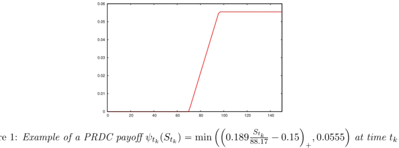
Remark 2.1. The financial products we consider in the applications are PRDC. Their payoffs (see Figure 1) have the following expression
ψtkpxq “ min ˜ maxˆ Cfptkq S0 x ´ Cdptkq, Floorptkq ˙ , Capptkq ¸ (2.4)
where Floorptkq and Capptkq are the floor and cap values chosen at the creation of the product,
as well as Cfptkq and Cdptkq that are the coupons value we wish to compare to the foreign and
the domestic currency, respectively.
0 0.01 0.02 0.03 0.04 0.05 0.06 0 20 40 60 80 100 120 140
Figure 1: Example of a PRDC payoff ψtkpStkq “ min
´´ 0.18988.17Stk ´ 0.15 ¯ `, 0.0555 ¯ at time tk.
The interesting feature of such functions is that their (right) derivative have a compact support.
2.2 Backward Dynamic Programming Principle
Vk can also be defined recursively by
$ & % Vn“ e´ ştn 0 r d sdsψ npStnq, Vk“ max ´ e´ ştk 0 rdsdsψ kpStkq,ErVk`1| Ftks ¯ , 0 ď k ď n ´ 1 (2.5)
and this representation is called the Backward Dynamic Programming Principle (BDPP). First, noticing that the obstacle process e´şt0rd
sdsψ
tpStq can be rewritten as a function ht of
two processes Xt and Yt such that
htpXt, Ytq “ e´ şt 0r d sdsψ tpStq
where h is given by htpx, yq “ ϕdptq e´yψt ˆ S0 ϕfptq ϕdptq e´σS2t{2`x`y ˙ (2.6) and pX, Y q is defined by pXt, Ytq “ ˆ σSWtS` σf żt 0 pt ´ sqdWsf, ´σd żt 0 pt ´ sqdWsd ˙ . (2.7)
Now, in order to alleviate notations, we denote by Xk “ Xtk, W
f k “ W f tk, Yk “ Ytk, W d k “ Wtdk, WkS“ WtSk and hk“ htk.
Using this new form, the Snell envelope becomes Vk “ sup
τ PTn k
E“hτpXτ, Yτq | Ftk
‰
and the Backward Dynamic Programming Principle (2.5) rewrites $ & % Vn“ hnpXn, Ynq, Vk “ max ´ hkpXk, Ykq,E“Vk`1| Ftks ¯ , 0 ď k ď n ´ 1. (2.8)
Second, in order to solve the problem theoretically by dynamic programming it is required to associate a Ft-Markov process to this problem and in our case, the simplest of them (i.e. of minimal dimension) is pXt, Wtf, Yt, Wtdq which is Ft-adapted and a Markov process because
$ ’ ’ ’ ’ ’ ’ ’ ’ ’ ’ ’ ’ ’ & ’ ’ ’ ’ ’ ’ ’ ’ ’ ’ ’ ’ ’ % Xk`1“ Xk` σfδWkf ` σS żtk`1 tk dWsS` σf żtk`1 tk ptk`1´ sqdWsf Wk`1f “ Wkf ` żtk`1 tk dWsf Yk`1“ Yk´ σdδWkd´ σd żtk`1 tk ptk`1´ sqdWsd Wk`1d “ Wkd` żtk`1 tk dWsd
where δ “ Tn and can be written as $ ’ ’ ’ ’ & ’ ’ ’ ’ % Xk`1 “ Xk` σfδWkf ` G1k`1 Wk`1f “ Wkf ` G2k`1 Yk`1 “ Yk´ σdδWkd` G3k`1 Wk`1d “ Wkd` G4k`1, (2.9)
where the increments are normally distributed ¨ ˚ ˚ ˝ G1k`1 G2k`1 G3 k`1 G4k`1 ˛ ‹ ‹ ‚„ N ´ µk`1, Σk`1 ¯ (2.10) with µk`1“ ¨ ˚ ˚ ˝ 0 0 0 0 ˛ ‹ ‹ ‚ and Σk`1“ ˆ Cov`Gik`1, G j k`1 ˘ ˙ i,j“1:4 . (2.11)
One notices that `pG1k, G2k, G3k, G4kq˘k“1...,n are i.i.d. Based on Equation (2.9), we deduce the Markov process transition of pXk, Wkf, Yk, Wkdq, for any integrable function f :R4 Ñ R, given
by
P f px, u, y, vq “ E“fpx ` σfδu ` G1k`1, u ` G2k`1, y ´ σdδv ` G3k`1, v ` G4k`1q‰. (2.12)
Remark 2.2. Using the Markov process pX, Wf, Y, Wdq newly defined, we rewrite the filtration Ftas
Ft“ σ`WS
s, Wsd, Wsf, s ď t
˘
“ σ`Xs, Wsf, Ys, Wsd, s ď t˘. (2.13)
Then, using the new expression for the filtration and the Markov property of pXk, Wkf, Yk, Wkdq,
the BDPP (2.8) reads as follows, $ & % Vn“ hnpXn, Ynq, Vk“ max ´ hkpXk, Ykq,E“Vk`1 | pXk, Wkf, Yk, Wkdq ‰¯ , 0 ď k ď n ´ 1. (2.14)
Moreover, by backward induction we get Vk“ vkpXk, Wkf, Yk, Wkdq where
$ & % vnpXn, Wnf, Yn, Wndq “ hnpXn, Ynq, vkpXk, Wkf, Yk, Wkdq “ max ´ hkpXk, Ykq, P vk`1pXk, Wkf, Yk, Wkdq ¯ , 0 ď k ď n ´ 1. (2.15) Payoff regularity. First, we look at the regularity of the payoff. The next proposition will then allow us to study the regularity of the value function through the propagation of the local Lipschitz property by the transition of the Markov process.
Proposition 2.3. If ψtk is are Lipschitz continuous with Lipschitz coefficient rψtksLip with
com-pactly supported (right) derivative (such as the payoff defined in (2.4)) then hkpx, yq given by (2.6) is locally Lipschitz continuous, for every x, x1, y, y1PR
|hkpx, yq ´ hkpx1, y1q| ď e|y|_|y 1|` r sψksLip|x ´ x 1 | ` pϕdptkq}ψtk}8` r sψksLipq|y ´ y 1 |˘ (2.16) with r sψksLip “ rψtksLipS0ϕfptkq e
´σS2tk{2}ψ1
tk}8e
c with ψ1
tk the right derivative of ψtk.
Proof. Let gk be defined by
gkpx, yq “ ψtk ˆ S0 ϕfptkq ϕdptkq e´σ2Stk{2`x`y ˙ . (2.17) As ψ1
tk has a compact support, then it exists c PR such that
|pψtkpe x qq1| “ | exψ1 tkpe x q| ď }ψ1tk}8 sup xPsupp ψ1 tk exď }ψt1k}8e c. (2.18) Hence |gkpx, yq ´ gkpx1, y1q| ď r sψksLip ϕdptkq ` |x ´ x1| ` |y ´ y1|˘ (2.19)
with r sψksLip “ rψtksLipS0ϕfptkq e
´σ2Stk{2}ψ1
tk}8e
c. Then for every x, x1, y, y1 PR, we have
|hkpx, yq ´ hkpx1, y1q| “ ϕdptkq ˇ ˇe´ygkpx, yq ´ e´y 1 gkpx1, y1q ˇ ˇ ď ϕdptkq ´ ˇ ˇe´ygkpx, yq ´ e´y 1 gkpx, yq ˇ ˇ` ˇ ˇe´u 1 gkpx, yq ´ e´y 1 gkpx1, y1q ˇ ˇ ¯ ď ϕdptkq ´ˇ ˇe´y´ e´y 1ˇ ˇ¨ }ψt k}8` e ´y1ˇ ˇgkpx, yq ´ gkpx1, y1q ˇ ˇ ¯ ď e|y|_|y1|`r sψksLip|x ´ x 1 | ` pϕdptkq}ψtk}8` r sψksLipq|y ´ y 1 |˘. (2.20)
The next Lemma shows that the transition of the Markov process propagates the local Lips-chitz continuity of a function f . This result will be helpful to estimate the error induced by the numerical approximation (2.15).
Lemma 2.4. Let P f px, u, y, vq “ E“fpx ` σfδu ` G1, u ` G2, y ´ σdδv ` G3, v ` G4q
‰ be a Markov kernel. If the function f satisfies the following local Lipschitz property,
|f px, u, y, vq ´ f px1, u1, y1, v1q| ď`A|x ´ x1| ` B|u ´ u1| ` C|y ´ y1| ` D|v ´ v1|˘ ˆ e|y|_|y1|`b|v|_|v1|
(2.21)
then
|P f px, u, y, vq ´ P f px1, u1, y1, v1q| ď`A|x ´ xr 1| ` rB|u ´ u1| ` rC|y ´ y1| ` rD|v ´ v1| ˘
ˆ e|y|_|y1|`rb|v|_|v1|.
(2.22)
Proof. It follows from Jensen’s inequality and our assumption on f |P f px, u, y, vq ´ P f px1, u1, y1, v1 q| ďE ”ˇ ˇf px ` σfδu ` G1, u ` G2, y ´ σdδv ` G3, v ` G4q ´ f px1` σfδu1` G1, u1` G2, y1´ σdδv1` G3, v1` G4q ˇ ˇ ı
ď`A|x ´ x1| ` pB ` Aσfδq|u ´ u1| ` C|y ´ y1| ` pD ` Cσdδq|v ´ v1|
˘
ˆ e|y|_|y1|`pb`σdδq|v|_|v1|E“ e|G3|`b|G4|‰
ď`A|x ´ xr 1| ` rB|u ´ u1| ` rC|y ´ y1| ` rD|v ´ v1| ˘
ˆ e|y|_|y1|`rb|v|_|v1|
(2.23)
where
r
A “ A Erκs, B “ pB ` Aσr fδq Erκs (2.24)
and
r
C “ C Erκs, D “ pD ` Cσr dδq Erκs, rb “ b ` σdδ (2.25) with κ “ expp|G3| ` b|G4|q andErκs ă `8.
Value function regularity. If the functions pψtkqk“0:n are defined as in Equation (2.4) then
vnpx, u, y, vq preserves a local Lipschitz property. Hence, for every x, x1, u, u1, y, y1, v, v1 PR,
|vnpx, u, y, vq ´ vnpx1, u1, y1, v1q| ď`An|x ´ x1| ` Bn|u ´ u1| ` Cn|y ´ y1| ` Dn|v ´ v1|
˘
ˆ e|y|_|y1|`bn|v|_|v1| (2.26)
where
An“ r sψnsLip, Bn“ 0, Cn“ ϕdptnq}ψn}8 ` r sψnsLip, Dn“ 0, bn“ 0 (2.27)
with r sψnsLip “ rψtnsLipS0ϕfptnq expp´σ
2
Stn{2q}ψt1n}8e
c. Using now Lemma 2.4 recursively and
have |vkpx, u, y, vq ´ vkpx1, u1, y1, v1q| ď max`|hkpx, yq ´ hkpx1, y1q|, |P vk`1px, u, y, vq ´ P vk`1px1, u1, y1, v1q| ˘ ď max ˆ e|y|_|y1|` r sψksLip|x ´ x 1 | ``ϕdptkq}ψtk}8 ` r sψksLip ˘ |y ´ y1|˘ ,`Ark|x ´ x1| ` rBk|u ´ u1| ` rCk|y ´ y1| ` rDk|v ´ v1| ˘ ˆ e|y|_|y1|`rbk|v|_|v1| ˙ ď`Ak|x ´ x1| ` Bk|u ´ u1| ` Ck|y ´ y1| ` Dk|v ´ v1| ˘ ˆ e|y|_|y1|`bk|v|_|v1| (2.28) where
Ak“ r sψksLip_`Ak`1Erκk`1s˘, Bk “ pBk`1` Ak`1σfδq Erκk`1s, bk“ bk`1` σdδ
(2.29) and
Ck“`ϕdptkq}ψtk}8` r sψksLip
˘
_`Ck`1Erκk`1s˘, Dk“ pDk`1` Ck`1σdδq Erκk`1s (2.30)
with κk`1“ expp|G3k`1| ` bk`1|G4k`1|q. Or equivalently
Ak “ max lěk ˆ r sψlsLip l ź j“k`1 Erκjs ˙ , Bk “ σf T n n ÿ l“k`1 max lďiďn ˆ r sψisLip i ź j“k`1 Erκjs ˙ (2.31) and Ck“ max lěk ˆ `ϕdptlq}ψl}8 ` r sψlsLip ˘ l ź j“k`1 Erκjs ˙ , Dk“ σd T n n ÿ l“k`1 max lďiďn ˆ `ϕdptiq}ψi}8` r sψisLip ˘ i ź j“k`1 Erκjs ˙ (2.32) with bk “ σdT ´ 1 ´k ´ 1 n ¯ . (2.33)
3
Bermudan pricing using Optimal Quantization
In this section, we propose two numerical solutions based on Product Optimal Quantization for the pricing of Bermudan options on the F X rate St. First, we remind briefly what is an optimal quantizer and what we mean by a product quantization tree. Second, we present a first numerical solution, based on quantization of the Markovian tuple pX, Wf, Y, Wdq, to solve the numerical problem (2.14) and detail the L2-error induced by this approximation. However, remember that we are looking for a method that makes possible to compute xVA’s risk mea-sures in a reasonable time but this solution can be too time consuming in practice due to the dimensionality of the quantized processes. That is why we present a second numerical solution which reduces the dimensionality of the problem by considering an approximate problem, based on quantization of the non-Markovian couple pX, Y q, introducing a systematic error induced by the non-markovianity and we study the L2-error produced by this approximation.
3.1 About Optimal Quantization
Theoretical background (the one-dimensional case). The aim of Optimal Quantization is to determine ΓN, a set with cardinality at most N , which minimises the quantization error
among all such sets Γ. We place ourselves in the one-dimensional case. Let Z be an R-valued random variable with distributionPZ defined on a probability space pΩ, A,Pq such that Z P L2R.
Definition 3.1. Let ΓN “ tz1, . . . , zNu ĂR be a subset of size N , called N -quantizer. A Borel
partition `CipΓNq
˘
iPJ1,N K ofR is a Voronoï partition of R induced by the N -quantizer ΓN if, for
every i “ t1, ¨ ¨ ¨ , N u, Ci`ΓN ˘ Ă ! ξ P R, |ξ ´ zi| ď min j‰i |ξ ´ zj| ) .
The Borel sets CipΓNq are called Voronoï cells of the partition induced by ΓN.
One can always consider that the quantizers are ordered: z1 ă z2ă ¨ ¨ ¨ ă zN ´1ă zN and in
that case the Voronoï cells are given by Ck`ΓN ˘ “`zk´1{2, zk`1{2‰, k PJ1, N ´ 1K, CN`ΓN ˘ “`zN ´1{2, zN `1{2 ˘
where @k P t2, ¨ ¨ ¨ , N u, zk´1{2“ zk´12`zk and z1{2“ inf` supppPZq
˘
and zN `1{2“ sup` supppPZq
˘ . Definition 3.2. Let ΓN “ tz1, . . . , zNu be an N -quantizer. The nearest neighbour projection
ProjΓN : R Ñ tz1, . . . , zNu induced by a Voronoï partition `CipΓNq
˘ iPt1,¨¨¨ ,N u is defined by @ξ PR, ProjΓNpξq “ N ÿ i“1 zi1ξPCipΓNq.
Hence, we can define the quantization of Z as the nearest neighbour projection of Z onto ΓN by
composing ProjΓ N and X p ZΓN “ Proj ΓNpZq “ N ÿ i“1 zi1ZPCipΓNq.
In order to alleviate notations, we write pZN from now on in place of pZΓN.
Now that we have defined the quantization of Z, we explain where does the term "optimal" comes from in the term optimal quantization. First, we define the quadratic distortion function. Definition 3.3. The L2-mean quantization error induced by the quantizer pZN is defined as
}Z ´ pZN}2 “ ˆ E ” min iPt1,¨¨¨ ,N u|Z ´ zi| 2ı ˙1{2 “ ˆ ż R min iPt1,¨¨¨ ,N u|ξ ´ zi| 2 PZpdξq ˙1{2 . (3.1)
It is convenient to define the quadratic distortion function at level N as the squared mean quadratic quantization error on pRqN:
Q2,N : z “`z1, . . . , zN ˘ ÞÝÑE ” min iPt1,¨¨¨ ,N u|Z ´ zi| 2ı “ }Z ´ pZN}22.
Remark 3.4. All these definitions can be extended to the Lp case. For example the Lp-mean quantization error induced by a quantizer of size N is
}Z ´ pZN}p “ ˆ E ” min iPt1,¨¨¨ ,N u|Z ´ zi| pı ˙1{p “ ˆ ż R min iPt1,¨¨¨ ,N u|Z ´ zi| p PZpdξq ˙1{p . (3.2)
The existence of a N -tuple zpN q“ pz
1, . . . , zNq minimizing the quadratic distortion function
Q2,N at level N has been shown and its associated quantizer ΓN “ tzi, i P t1, ¨ ¨ ¨ , N uu is called
an optimal quadratic N -quantizer, see e.g. [Pag18] for further details and references. We now turn to the asymptotic behaviour in N of the quadratic mean quantization error. The next Theorem, known as Zador’s Theorem, provides the sharp rate of convergence of the Lp-mean quantization error.
Theorem 3.5. (Zador’s Theorem) Let p P p0, `8q.
(a) Sharp rate. Let Z P Lp`δR pPq for some δ ą 0. Let PZpdξq “ ϕpξq ¨ λpdξq ` νpdξq, where
ν K λ i.e. denotes the singular part of PZ with respect to the Lebesgue measure λ on R.
Then, lim N Ñ`8NΓNĂR,|ΓminN|ďN }Z ´ pZN}p “ 1 2ppp ` 1q „ ż R ϕ1`p1 dλ 1`1 p . (3.3)
(b) Non asymptotic upper-bound. Let δ ą 0. There exists a real constant C1,p,δ P p0, `8q
such that, for every R-valued random variable Z,
@N ě 1, min
ΓNĂR,|ΓN|ďN
}Z ´ pZN}pď C1,p,δσδ`ppZqN
´1 (3.4)
where, for r P p0, `8q, σrpZq “ minaPR}Z ´ a}r ă `8.
The next result answers to the following question: what can be said about the convergence rate ofE“|Z ´ pZN|2`β‰, knowing that pZN is a quadratic optimal quantization?
This problem is known as the distortion mismatch problem and has been first addressed by [GLP08] and the results have been extended in Theorem 4.3 of [PS18].
Theorem 3.6. [Lr-Ls-distortion mismatch] Let Z : pΩ, A,Pq Ñ R be a random variable and let r P p0, `8q. Assume that the distribution PZ of Z has a non-zero absolutely continuous
component with density ϕ. Let pΓNqN ě1 be a sequence of Lr-optimal grids. Let s P pr, r ` 1q. If
Z P L1`r´ss `δpΩ, A,Pq (3.5)
for some δ ą 0, then
lim sup
N
N }Z ´ pZN}s ă `8. (3.6)
Product Quantization. Now, let Z “ pZ`q`“1:d be an Rd-valued random vector with
dis-tribution PZ defined on a probability space pΩ, A,Pq. There are two approaches if one wishes to scale to higher dimensions. Either one applies the above framework directly to the random vector Z and build an optimal quantizer of Z, or one may consider separately each component Z` independently, build a one-dimensional optimal quantization pZ`, of size N`, with quantizer ΓN` ` “ z`i`, i` P t1, ¨ ¨ ¨ , N
`
u( and then build the product quantizer ΓN “ śd`“1ΓNl ` of size N “ N1ˆ ¨ ¨ ¨ ˆ Nd defined by ΓN “ pz1i1, ¨ ¨ ¨ , z ` i`, ¨ ¨ ¨ , z d idq, i`P t1, ¨ ¨ ¨ , N`u, ` P t1, ¨ ¨ ¨ , du(. (3.7)
In our case we chose the second approach. Indeed, it is much more flexible when dealing with normal distribution, like in our case. We do not need to solve the d-dimensional minimization problem at each time step. We only need to load precomputed optimal quantizer of standard normal distribution N p0, 1q and then take advantage of the stability of optimal quantization by
rescaling in one dimension in the sense that if ΓN “ tzi, 1 ď i ď N u is optimal at level N for
N p0, 1q then µ ` σΓN (with obvious notations) is optimal for N pµ, σ2
q.
Even though it exists fast methods for building optimal quantizers in two-dimension based on deterministic methods like in the one-dimensional case, when dealing with optimal quantization of bivariate Gaussian vector, we may face numerical instability when the covariance matrix is ill-conditioned: so is the case if the variance of one coordinate is relatively high compared to the second one (which is our case in this paper). This a major drawback as we are looking for a fast numerical solution able to produce prices in a few seconds and this is possible when using product optimal quantization.
Quantization Tree. Now, in place of considering a random variable Z, let pZtqtPr0,T s be a
stochastic process following a Stochastic Differential Equation (SDE)
Zt“ Z0` żt 0 bspZsqds ` żt 0 σps, ZsqdWs (3.8)
with Z0 “ z0 PRd, W a standard Brownian motion living on a probability space pΩ, A,Pq and
b and σ satisfy the standard assumptions in order to ensure the existence of a strong solution of the SDE.
What we call Quantization Tree is defined, for chosen time steps tk“ T k{n, k “ 0, ¨ ¨ ¨ , n, by quantizers pZkof Zk(Product Quantizers in our case) at dates tkand the transition probabilities
between date tk and date tk`1. Although p pZkqk is no longer a Markov process we will consider
the transition probabilities πijk “ Lp pZk`1 | pZkq. We can apply this methodology because, with
the model we consider, we know all the marginal laws of our processes at each date of interest. In the next subsection, we present the approach based on the quantization tree previously defined that allows us to approximate the price of Bermudan options where the risk factors are driven by the 3-factor model (1.1).
3.2 Quantization tree approximation: Markov case
Our first idea in order to discretize (2.14) is to replace the processes by a product quantizer composed with optimal quadratic quantizers. Indeed, at each time tk, we know the law of the
processes Xk, Wkf, Yk and Wkd. Then we "force" in some sense the (lost) Markov property by introducing the Quantized Backward Dynamic Programming Principle (QBDPP) defined by
$ & % p Vn“ hnp pXn, pYnq, p Vk“ max ´ hkp pXk, pYkq,E “ p Vk`1| p pXk, xWkf, pYk, xWkdq ‰¯ , 0 ď k ď n ´ 1, (3.9) where for every k “ 0, . . . , n, pXk, xWkf, pYkand xWkdare quadratic optimal quantizers of Xk, Wkf, Yk
and Wkdof size NkX, NkWf, NkY and NkWdrespectively and we denote Nk“ NkXˆNW
f
k ˆNkYˆNW
d
k
the size of the grid of the product quantizer.
We are interested by the error induced by the numerical algorithm defined in (3.9) and more precisely its L2-error, with in mind that we "lost" the Markov property in the quantization procedure. Moreover, this can be circumvented as shown below.
Theorem 3.7. Let the Markov transition P f px, u, y, vq defined in (2.12) be locally Lipschitz in the sense of Lemma 2.4. Assume that all the payoff functions pψtkqk“0:n are Lipschitz
approximation p pXk, xWkf, pYk, xWkdq is upper-bounded by › ›Vk´ pVk › › 2 ď ˆ n ÿ l“k CXl › ›Xl´ pXl › › 2 2p` CYl › ›Yl´ pYl › › 2 2p` CWld › ›Wld´ xWld › › 2 2p` CWlf › ›Wlf ´ xWlf › › 2 2p ˙1{2 , (3.10) where 1 ă p ă 3{2 and q ě 1 such that 1p`1q “ 1 and
CXl“ r sψls 2 Lip › ›e|Yl|_| pYl| › › 2 2q` rA 2 lKl2, CWd l “ rB 2 lKl2, CYl“`ϕdptlq}ψtl}8` r sψlsLip ˘2› ›e|Yl|_| pYl| › › 2 2q` rC 2 lKl2, CWlf “ rD 2 lKl2 (3.11) with Kl “ › ›e|Yl|_| pYl|`rbl|W d l|_|xWld|›› 2q. (3.12)
As a consequence if sN “ min Nk, we have
lim s N Ñ`8 › ›Vk´ pVk › › 2 2 “ 0. (3.13)
Remark 3.8. From the definition of the processes Xk, Wkf, Ykand Wkd, all are Gaussian random variables hence all the L2q-norms in Equations (3.11) and (3.12) are finite. Indeed, let Z „
N p0, σZq a Gaussian random variable with variance σ
2
Z and pZ an optimal quantizer of Z with
cardinality N then @λ PR` › ›eλ|Z|_| pZ| › › 2q “ ˆ E“ e2qλ|Z|_| pZ|‰ ˙1 2q ď ˆ 2 E“ e2qλ|Z|‰ ˙1 2q ď 2 1 2qeq 2λ2σ2 Z. (3.14)
Proof. The error between the Snell envelope and its approximation is given by |Vk´ pVk| ď max ´ˇ ˇhkpXk, Ykq ´ hkp pXk, pYkq ˇ ˇ, ˇ ˇE“Vk`1| pXk, Wf k, Yk, W d kq ‰ ´E“Vpk`1 | p pXk, xWf k, pYk, xW d kq ‰ˇ ˇ ¯ (3.15) thus, using the local Lipschitz property of hkestablished in Proposition 2.3 and Hölder’s inequal-ity with p, q ě 1 such that 1p `1q “ 1, the L2-error is upper-bounded by
› ›Vk´ pVk › › 2 2 ď › ›hkpXk, Ykq ´ hkp pXk, pYkq › › 2 2 `››E“Vk`1 | pXk, Wf k, Yk, W d kq ‰ ´E“Vpk`1 | p pXk, xWf k, pYk, xW d kq ‰› › 2 2. ď››e|Yk|_| pYk| › › 2 2q ´ `ϕdptkq}ψtk}8` r sψksLip ˘2› ›Yk´ pYk › › 2 2p` r sψks 2 Lip › ›Xk´ pXk › › 2 2p ¯ `››E“Vk`1| pXk, Wf k, Yk, W d kq ‰ ´E“Vpk`1| p pXk, xWf k, pYk, xW d kq ‰› ›2 2. (3.16) Looking at the last term, we have
E“Vk`1| pXk, Wkf,Yk, Wkdq ‰ ´E“Vpk`1 | p pXk, xWf k, pYk, xW d kq ‰ “E“Vk`1 | pXk, Wkf, Yk, Wkdq ‰ ´E“Vk`1| p pXk, xWkf, pYk, xWkdq ‰ `E“Vk`1 | p pXk, xWkf, pYk, xWkdq ‰ ´E“Vpk`1| p pXk, xWf k, pYk, xW d kq ‰ q. (3.17)
• For the first term, notice that E“Vk`1 | pXk, Wkf, Yk, Wkdq ‰ “ P vk`1pXk, Wkf, Yk, Wkdq (3.18) and E“Vk`1 | p pXk, xWkf, pYk, xWkdq ‰ “ P vk`1p pXk, xWkf, pYk, xWkdq (3.19)
then, we directly apply Lemma 2.4 on the function vk`1 and obtain
|P vk`1pXk, Wkf, Yk, Wkdq ´ P vk`1p pXk, xWkf, pYk, xWkdq| ď ´ r Ak|Xk´ pXk| ` rBk|Wkf ´ xW f k| ` rCk|Yk´ pYk| ` rDk|Wkd´ xWkd| ¯ e|Yk|_| pYk|`rbk|Wkd|_|xW d k| (3.20) with rAk, rBk, rCk, rDk and rbk defined by (2.24) and (2.25). Hence, using Hölder’s inequality with
p, q ě 1 such that 1p `1q “ 1, › ›E“Vk`1| pXk, Wf k, Yk, W d kq ‰ ´E“Vk`1| p pXk, xWkf, pYk, xWkdq ‰› › 2 2 ď ´ r A2k››Xk´ pXk › › 2 2p` rB 2 k › ›Wf k ´ xW f k › › 2 2p ` rC 2 k › ›Yk´ pYk › › 2 2p` rD 2 k › ›Wkd´ xWkd › › 2 2p ¯ ˆ››e|Yk|_| pYk|`rbk|W d k|_|xWkd|››2 2q. (3.21)
• The last one is useful for the induction, indeed › ›E“Vk`1| p pXk, xWf k, pYk, xW d kq ‰ ´E“Vpk`1 | p pXk, xWf k, pYk, xW d kq ‰› › 2 2 ď › ›Vk`1´ pVk`1 › › 2 2. (3.22)
Finally, using the Lr-Ls mismatch theorem for the quadratic optimal quantizers pXk and pYk,
if 1 ă p ă 3{2, then lim sup NX k NkX}Xk´ pXk}2p ă `8, lim sup NY k NkY}Yk´ pYk}2p ă `8, lim sup NW f k
NkWf}Wkf ´ xWkf}2p ă `8 and lim sup
NW d k NkWd}Wkd´ xWkd}2p ă `8 (3.23) this yields › ›Vk´ pVk › › 2 2 ď››Xk´ pXk › › 2 2p ´ r sψks2Lip › ›e|Yk|_| pYk| › › 2 2q` rA 2 kKk2 ¯ `››Yk´ pYk › › 2 2p ´ `ϕdptkq}ψtk}8` r sψksLip ˘2› ›e|Yk|_| pYk| › › 2 2q` rC 2 kKk2 ¯ ` rBk2Kk2››Wkf ´ xWkf › › 2 2p ` rD 2 kKk2 › ›Wkd´ xWkd › › 2 2p` › ›Vk`1´ pVk`1 › › 2 2 ď n ÿ l“k CXl › ›Xl´ pXl › › 2 2p` CYl › ›Yl´ pYl › › 2 2p` CWld › ›Wld´ xWld › › 2 2p` CWlf › ›Wlf ´ xWlf › › 2 2p s N Ñ`8 ÝÝÝÝÝÑ 0 (3.24) where Kk“››e|Yk|_| pYk|`rbk|W d k|_|xWkd|›› 2q and @k “ 1, . . . , n, CXk, CYk, CWkd, CWkf ă `8.
Remark 3.9. The same result can be obtained if we relax the assumption on the payoff ψk. If we only assume the payoff Lipschitz continuous, we have the same limit with the same rate of convergence, however the constants CXl, CYl, CWd
l, CW f l
To conclude this section, although considering product optimal quantizer in four dimensions for pXk, Wkf, Yk, Wkdq seems to be natural, the computational cost associated to the resulting
QBDPP is too high, of order Opn ˆ pmax Nkq2q. Moreover the computation of the transition
probabilities needed for the evaluation of the termsE“Vpk`1 | p pXk, xWf
k, pYk, xW d kq
‰
are challenging. These transition probabilities cannot be computed using deterministic numerical integration methods and we have to use Monte Carlo estimators. Even though it is feasible, it is a drawback for the method since it increases drastically the computation time for calibrating the quantization tree. In the next section we provide a solution to these problems which consists in reducing the dimension of the problem at the price of adding a systematic error, which turns out to be quite small in practice.
3.3 Quantization tree approximation: Non Markov case
In this part, we want to reduce the dimension of the problem in order to scale down the numerical complexity of the pricer. For that we discard the processes Wdand Wf in the tree and only keep X and Y . Doing so, we loose the Markovian property of our original model but we drastically reduce the numerical complexity of the problem. Thence, (2.14) is approximated by
$ & % p Vn“ hnp pXn, pYnq, p Vk“ max ´ hkp pXk, pYkq,E “ p Vk`1| p pXk, pYkq ‰¯ , 0 ď k ď n ´ 1 (3.25)
where for every k “ 0, . . . , n, pXk and pYk are quadratic optimal quantizers of Xk and Yk of size
NkX and NkY, respectively and we denote Nk “ NkX ˆ NkY the size of the grid of the product
quantizer.
Theorem 3.10. Let the Markov transition P f px, u, y, vq be defined by (2.12) be locally Lipschitz in the sense of Lemma 2.4. Assume that all the payoff functions pψtkqk“0:n are Lipschitz
contin-uous with compactly supported (right) derivative. Then the L2-error, induced by the quantization approximation p pXk, pYkq is upper-bounded by › ›Vk´ pVk › › 2 ď ˆn´1 ÿ l“k CWf l`1 › ›Wl`1f ´ErWl`1f | pXl, Ylqs › › 2 2p` CWl`1d › ›Wl`1d ´ErWl`1d | pXl, Ylqs › › 2 2p ` CXl › ›Xl´ pXl › › 2 2p ` CYl › ›Yl´ pYl › › 2 2p ˙1{2 (3.26) where 1 ă p ă 3{2 and q ě 1 such that 1p`1q “ 1, moreover
CXl “ r sψls 2 Lip › ›e|Yl|_| pYl| › › 2 2q` sA 2 l › ›e s bl|Yl|_| pYl|› › 2 2q, CWl`1f “ B 2 l`1 › ›rκk`1 › › 2 2q, CYl “`ϕdptlq}ψtl}8` r sψlsLip ˘2› ›e|Yl|_| pYl| › › 2 2q` sC 2 l › ›esbl|Yl|_| pYl| › › 2 2q, CWl`1d “ D 2 l`1 › ›rκk`1 › › 2 2q. (3.27) Taking the limit in sN “ min Nk, the size of the quadratic optimal quantizers, we have
lim s N Ñ`8 › ›Vk´ pVk › › 2 2 “ n´1 ÿ l“k CWf l`1 › ›Wf l`1´ErW f l`1 | pXl, Ylqs › › 2 2p`CWl`1d › ›Wl`1d ´ErWl`1d | pXl, Ylqs › › 2 2p. (3.28) Proof. We apply the same methodology as in the proof for the Markov case. The error between the Snell envelope and its approximation is given by
|Vk´ pVk| ď max ´ ˇ ˇhkpXk, Ykq ´ hkp pXk, pYkq ˇ ˇ, ˇ ˇE“Vk`1| pXk, Wf k, Yk, W d kq ‰ ´E“Vpk`1| p pXk, pYkq ‰ˇ ˇ ¯ (3.29)
thus, using Proposition 2.3 and Hölder’s inequality with p, q ě 1 such that 1p`1q “ 1, the L2-error is given by › ›Vk´ pVk › › 2 2 ď › ›hkpXk, Ykq ´ hkp pXk, pYkq › › 2 2 `››E“Vk`1 | pXk, Wf k, Yk, W d kq ‰ ´E“Vpk`1| p pXk, pYkq ‰› › 2 2 ď ´ r sψks2Lip › ›Xk´ pXk › › 2 2p ``ϕdptkq}ψtk}8 ` r sψksLip ˘2› ›Yk´ pYk › › 2 2p ¯› ›e|Yk|_| pYk| › › 2 2q `››E“Vk`1| pXk, Wkf, Yk, Wkdq ‰ ´E“Vpk`1 | p pXk, pYkq ‰› › 2 2. (3.30) The last term in Equation (3.30) can be decomposed as follows
E“Vk`1 | pXk, Wkf, Yk, Wkdq ‰ ´E“Vpk`1 | p pXk, pYkq ‰ “E“Vk`1 | pXk, Wkf, Yk, Wkdq ‰ ´E“Vk`1 | pXk, Ykq ‰ `E“Vk`1 | pXk, Ykq ‰ ´E“Vk`1| p pXk, pYkq ‰ `E“Vk`1 | p pXk, pYkq ‰ ´E“Vpk`1| p pXk, pYkq‰. (3.31)
And again, each term can be upper-bounded.
• The first can be upper-bounded using what we did above on the value function vkand Hölder’s
inequality with p, q ě 1 such that 1p `1q “ 1
› ›E“Vk`1 | pXk, Wf k, Yk, W d kq ‰ ´E“Vk`1| pXk, Ykq ‰› › 2 2 ď››Vk`1´E“Vk`1 | pXk, Ykq ‰› › 2 2 ď››vk`1pXk`1, Wf k`1, Yk`1, W d k`1q ´ vk`1`Xk`1, E“Wk`1f | pXk, Ykq‰, Yk`1, E“Wk`1d | pXk, Ykq ‰˘› › 2 2 ď › › › ´ Bk`1 ˇ ˇWk`1f ´E“Wk`1f | pXk, Ykq ‰ˇ ˇ` Dk`1 ˇ ˇWk`1d ´E“Wk`1d | pXk, Ykq ‰ˇ ˇ ¯ r κk`1 › › › 2 2 ď›› r κk`1 › ›2 2q ´ Bk`12 ››Wf k`1´ErW f k`1| pXk, Ykqs › ›2 2p` D 2 k`1 › ›Wk`1d ´E“Wk`1d | pXk, Ykq ‰› ›2 2p ¯ (3.32) with coefficients bk`1, Bk`1 and Dk`1 defined in (2.31) and (2.32) and
r κk`1“ e|Yk`1|`bk`1|W d k`1|_|ErW d k`1|pXk,Ykqs|. (3.33)
• For the second, we define r
vkpXk, Ykq “E“vk`1pXk`1, Wk`1f , Yk`1, Wk`1d q | pXk, Ykq‰. (3.34)
Indeed, E“Vk`1| pXk, Ykq
‰
is only a function of Xk and Yk, as shown below
E“Vk`1 | pXk, Ykq ‰ “E“vk`1pXk`1, Wk`1f , Yk`1, Wk`1d q | pXk, Ykq ‰ “E ” E“vk`1pXk`1, Wk`1f , Yk`1, Wk`1d q | pXk, Wkf, Yk, Wkdq ‰ | pXk, Ykq ı “E“P vk`1pXk, Wkf, Yk, Wkdq | pXk, Ykq‰. (3.35) Moreover, we can rewrite Wkf “ λkXk
KK ` ξk and Wkd“ rλkYk KK ` χk where λk “ CovpXk, Wkfq VarpXkq , rλk “ CovpYk , Wd kq VarpYkq
and ξk„ N p0, σξ2kq and χk „ N p0, σ2χkq with σ 2 ξk “VarpW f k´λkXkq and σχ2k “VarpW d k´rλkYkq, then E“P vk`1pXk, Wkf, Yk, Wkdq | pXk, Ykq “ px, yq ‰ “E“P vk`1px, λkx ` ξk, y, rλky ` χkq ‰ˇ ˇ px,yq“pXk,Ykq (3.36) yielding r vkpx, yq “E“P vk`1px, λkx ` ξk, y, rλky ` χkq‰. (3.37)
Now, using Lemma 2.4 onvrk, we have
ˇ ˇrvkpx, yq ´rvkpx1, y1q ˇ ˇ “ ˇ ˇ ˇ E“P vk`1px, λkx ` ξk, y, rλky ` χkq ´ P vk`1px 1, λ kx1` ξk, y1, rλky1` χkq ‰ˇˇ ˇ ďE „ ˇ ˇ ˇ ` p rAk` rBk|λk|q|x ´ x1| ` p1 ` rCk|rλk|q|y ´ y1|˘ ep1`rbk|rλk|q|y|_|y 1|`rb k|χk| ˇ ˇ ˇ ď ´ s Ak|x ´ x1| ` sCk|y ´ y1| ¯ esbk|y|_|y1| (3.38) where s Ak “ p rAk` rBk|λk|qE“ erbk|χk|‰, Csk“ 1 ` rCk|rλk|, (3.39) sbk“ 1 ` rbk|rλk| (3.40)
with rAk, rBk, rCk and rbk defined in (2.24) and (2.25). Hence, using Hölder’s inequality with
p, q ě 1 such that 1p `1q “ 1 › ›E“Vk`1| pXk, Ykq ‰ ´E“Vk`1| p pXk, pYkq ‰› › 2 2 “››rvkpXk, Ykq ´rvkp pXk, pYkq › › 2 2 ď › › › ´ s Ak ˇ ˇXk´ pXk ˇ ˇ` sCk ˇ ˇYk´ pYk ˇ ˇ ¯ esbk|Yk|_| pYk| › › › 2 2 ď››e sbk|Yk|_| pYk|› › 2 2q ´ s A2k››Xk´ pXk › › 2 2p` sC 2 k › ›Yk´ pYk › › 2 2p ¯ . (3.41)
• The last one is useful for the induction, indeed › ›E“Vk`1 | p pXk, pYkq ‰ ´E“Vpk`1| p pXk, pYkq ‰› › 2 2 ď › ›Vk`1´ pVk`1 › › 2 2. (3.42)
Finally, using the Lr-Ls mismatch theorem on the quadratic optimal quantizers pXk and pYk,
if 1 ă p ă 3{2, then lim sup
NX k
NkX}Xk´ pXk}2p ă `8 and lim sup
NY k
and › ›Vk´ pVk › › 2 2 ď››Xk´ pXk › › 2 2p ´ r sψks2Lip › ›e|Yk|_| pYk| › › 2 2q` sA 2 k › ›esbk|Yk|_| pYk| › › 2 2q ¯ `››Yk´ pYk › › 2 2p ´ `ϕdptkq}ψtk}8 ` r sψksLip ˘2› ›e|Yk|_| pYk| › › 2 2q` sC 2 k › ›e s bk|Yk|_| pYk|› › 2 2q ¯ ` B2k`1››κrk`1 › › 2 2q › ›Wf k`1´ErW f k`1 | pXk, Ykqs › › 2 2p ` Dk`12 › ›rκk`1 › › 2 2q › ›Wk`1d ´E“Wk`1d | pXk, Ykq ‰› › 2 2p ` › ›Vk`1´ pVk`1 › › 2 2 ď n´1 ÿ l“k CWf l`1 › ›Wl`1f ´ErWl`1f | pXl, Ylqs › › 2 2p` CWl`1d › ›Wl`1d ´ErWl`1d | pXl, Ylqs › › 2 2p ` CXl › ›Xl´ pXl › › 2 2p` CYl › ›Yl´ pYl › › 2 2p s N Ñ`8 ÝÝÝÝÝÑ n´1 ÿ l“k CWf l`1 › ›Wf l`1´ErW f l`1| pXl, Ylqs › › 2 2p ` CWl`1d › ›Wl`1d ´ErWl`1d | pXl, Ylqs › › 2 2p. (3.44)
Practitioner’s corner. Market implied values of σf, σd and σS used for the numerical com-putations are usually of order
σf « 0.005, σd« 0.005, σS « 0.5 (3.45)
and in the most extreme cases, we compute Bermudan options on foreign exchange with maturity 20 years (T “ 20). Thus, we can estimate the order of the induced systematic error. First, we recall the expression of the related coefficients which depends of
Bk“ σf T n n ÿ l“k`1 max lďiďn ˆ r sψisLip i ź j“k`1 Erκjs ˙ , Dk“ σd T n n ÿ l“k`1 max lďiďn ˆ pϕdptiq}ψi}8` r sψisLipq i ź j“k`1 Erκjs ˙ (3.46) with κj “ e|G 3 j|`bj|G4j|, r κl`1 “ e|Yl`1|`bl`1|W d l`1|_|ErWl`1d |pXl,Ylqs| (3.47) and bk“ σdT ˆ 1 ´k ´ 1 n ˙ . (3.48)
Now, considering the case where the payoffs are the same at each exercise date, the Lipschitz constants can be upper-bounded by r sψsLip:
r sψksLip “ rψtksLipS0ϕfptkq e ´σS2tk{2}ψ1 tk}8e c ď S0rψtksLip}ψ 1 tk}8e c “: r sψsLip (3.49) and let κ defined by
κ “ max k Erκks “E“ e |G30|`b0|G40|‰ď 1 2E“ e 2|G3 0|` e2b0|G40|‰ (3.50)
moreover, if Z „ N p0, σ2q thenE“ eλ|Z|‰“ eλ2σ2{2, thence we can upper-bound κ
κ ď 1 2E“ e σ2 3{2` eb20{2‰“ 1 2E“ e σ2 d{96` eσd2T2{2‰« 1. (3.51)
κ being bounded, we notice that the main constants Bk2 and Dk2 in the remaining error are of order σd2 or σf2, indeed Bkď σf T nr sψsLippn ´ kqκ n´k « σf T nr sψsLippn ´ kq, Dkď σd T n` maxl ϕdptlq}ψ}8 ` r sψsLip ˘ pn ´ kqκn´k « σd T np}ψ}8 ` r sψsLipqpn ´ kq. (3.52) Furthermore E“rκ 2q k`1 ‰ “E ” e2q|Yk`1|`2qbk`1|Wk`1d |_|ErW d k`1|pXk,Ykqs| ı ď 1 2 ˆ E ” e4q|Yk`1| ı `E ” e4qbk`1|Wk`1d |_|ErWk`1d |pXk,Ykqs| ı˙ ď 1 2 ˆ E ” e4q|Yk`1| ı `E ” e4qσdpT ´tkq|Wk`1d |_|ErWk`1d |pXk,Ykqs| ı˙ ď 1 2 ˆ e8q2σ2dT3{3`2 e8q2σd2pT ´tkq2tk`1 ˙ (3.53)
and from elementary inequality pa ` bq1{q ď a1{q` b1{q, a, b ě 0, q ě 1
› ›rκk`1 › › 2 2q “E “ r κ2qk`1‰1q ďˆ 1 2e 8q2σ2 dT3{3` e8q2σ2dpT ´tkq2tk`1 ˙1 q ďˆ 1 2e 8q2σ2 dT3{3 ˙1 q ` ˆ e8q2σ2dpT ´tkq2tk`1 ˙1 q ď 1 21{q e 8qσ2 dT3{3` e8qσ2dpT ´tkq2tk`1. (3.54)
The two terms on the right-hand side of the inequality do not explode. Indeed, the function g : t ÞÑ pT ´ tq2t, defined for t P r0, T s with T “ 20, attains its maximum on t “ 20{3 and gp20{3q « 1185, hence for the considered values
@k “ 1, . . . , n, ››rκk`1 › ›
2
2q ď Crκ« 6. (3.55)
informations in (3.28) we have › ›Vk´ pVk › ›2 2 N Ñ`8 ÝÝÝÝÝÑ n´1 ÿ l“k Bl`12 ›› r κl`1 › ›2 2q › ›Wl`1d ´ErWl`1d | pXl, Ylqs › ›2 2p ` Dl`12 ››rκl`1 › › 2 2q › ›Wf l`1´ErW f l`1| pXl, Ylqs › › 2 2p ďσf2 ´T n ¯2 r sψs2Lip n´1 ÿ l“k pn ´ lq2κ2pn´lqC r κ › ›Wl`1d ´ErWl`1d | pXl, Ylqs › › 2 2p ` σd2 ´T n ¯2 ` max l ϕdptlq}ψ}8` r sψsLip ˘2 ˆ n´1 ÿ l“k pn ´ lq2κ2pn´lqCrκ › ›Wl`1f ´ErWl`1f | pXl, Ylqs › › 2 2p ď2σ2f ´T n ¯2 r sψs2Lip n´1 ÿ l“k pn ´ lq2κ2pn´lqCκr › ›Wl`1d › › 2 2p ` 2σ2d ´T n ¯2 ` max l ϕdptlq}ψ}8` r sψsLip ˘2 n´1 ÿ l“k pn ´ lq2κ2pn´lqCrκ › ›Wf l`1 › › 2 2p ď ´ σf2r sψs2 Lip` σ 2 d` maxl ϕdptlq}ψ}8 ` r sψsLip ˘2¯ 4 Crκ π1{3 ´T n ¯2n´1ÿ l“k tl`1pn ´ lq2κ2pn´lq. (3.56) Hence, the systematic error is upper-bounded by the squared volatilities σd2 and σf2. These parameters being of order 5 ˆ 10´3 at most, the systematic error is negligible as long as these
volatilities stay reasonably small.
Remark 3.11. As in the Markov case, we can extend this result to the case where the payoffs pψkqk are Lipschitz continuous, however the residual error can not be as easily estimated and
controlled.
4
Numerical experiments
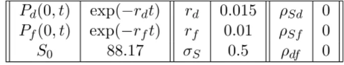
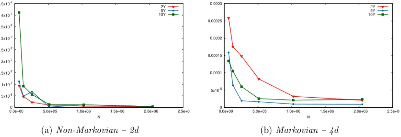
In this section, we illustrate the theoretical results found in Section 3 regarding the pricing of Bermudan options in the 3-factor model described in Section 1. First, we detail both algorithms and how to compute the quantities that appear in them (conditional expectation, conditional probabilities, ...). Then, we test our two numerical solutions for the pricing of European options, whose price is known in closed form. European options are Bermudan options with only one date of exercise, hence when using the non-Markovian approximate we do not introduce the systematic error shown in Theorem 3.10 but pricing these kind of options is a good benchmark in order to test our methodologies. Finally, we evaluate Bermudan options and compare our two solutions, the Markovian and the non-Markovian approximation.
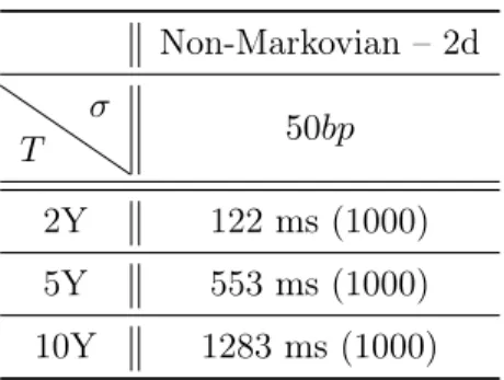
We have to keep in mind that the computation time is crucial because these pricers are only a small block in the complex computation of xVA’s. Indeed, they will be called hundreds of thousands of time each time these risks measures are needed.
All the numerical tests have been carried out in C++ on a laptop with a 2,4 GHz 8-Core Intel Core i9 CPU. The computations of the transition probabilities and the computations of the conditional expectations are parallelized on the CPU.
Remark 4.1. The computation times given below measure the time needed for loading the pre-computed optimal grids from files, rescaling the optimal quantizers in order to get the right
variance, computing the conditional probabilities (the part that demands the most in term of computing power) and finally computing the expectations for the pricing. One has to keep in mind that the complexity is linear in function of n, the number of exercise dates. Indeed, if we double the number of exercise dates, we double the number of conditional probability matrices and expectations to compute.
Characterisation of the Quantization Tree. In what follows, we describe the choice of parameters we made when building the quantization tree: the time discretisation and the size of each grid at each time.
• The time discretisation is an easy choice because it is decided by the characteristics of the financial product. Indeed, we take only one date (and today’s date) in the tree if we want to evaluate European options and if we want to evaluate Bermudan options we take as many discretisation dates (plus today’s date) in the tree as there are exercise dates in the description of the product.
• Then, we have to decide the size of each grid at each date in the tree. In our case, we consider grids of same size at each date hence Nk “ N, k “ 1 . . . , n and then we take
NX “ 10NY for both trees. This choice seems to be reasonable because the risk factor Xk is prominent, due to the value of σS compare to σd. Now, in the Markovian case, we
take NX “ 4NWf and NY “ 4NWd, indeed the two Brownian Motions are important
only when we compute the conditional expectation but not when we want to evaluate the payoffs, hence we want to give as much as possible of the budget N to NX and NY.
The algorithm: Markovian Case. Let pxki1qi1“1:NX, pu
k i2qi2“1:NW f, py k i3qi3“1:NY and pv k i4qi4“1:NW d
be the associated centroids of pXk, xWkf, pYkand xWkdrespectively, at a given time tkwith 0 ď k ď n.
Using the discrete property of the optimal quantizers, the conditional expectation appearing in (3.9) can be rewritten as E“Vpk`1| p pXk, xWf k, pYk, xW d kq “`xki1, u k i2, y k i3, v k i4 ˘‰ “E“pvk`1p pXk`1, xW f k`1, pYk`1, xWk`1d q | p pXk, xWkf, pYk, xWkdq “`xki1, u k i2, y k i3, v k i4 ˘‰ “ ÿ j1,j2,j3,j4 πi,j(m),kpvk`1`x k`1 j1 , u k`1 j2 , y k`1 j3 , v k`1 j4 ˘ (4.1)
where π(m),ki,j , with i “ pi1, i2, i3, i4q and j “ pj1, j2, j3, j4q, is the conditional probability defined
by π(m),ki,j “P ´ ` p Xk`1, xWk`1f , pYk`1, xWk`1d ˘ “`xk`1j1 , uk`1j 2 , y k`1 j3 , v k`1 j4 ˘ |`Xpk, xWkf, pYk, xWkd ˘ “`xki1, u k i2, y k i3, v k i4 ˘¯ .
Due to the dimension of the problem (4 in this case), we cannot compute these probabilities using deterministic methods, hence one has to simulate trajectories of the processes in order to evaluate them. We refer the reader to [BPP05, BP03, PPP04] for details on the methodology.
A way to reduce the complexity of the problem is to approximate these probabilities byrπi,j(m),k, where the conditional part `Xpk, xWkf, pYk, xWkd
˘ “`xki1, uki2, yik3, vik4˘(is replaced by pXk, Wkf, Yk, Wkdq “ `xk i1, u k i2, y k i3, v k i4 ˘( , yielding r πi,j(m),k“P ´ ` p Xk`1, xWk`1f , pYk`1, xWk`1d ˘ “`xk`1j1 , uk`1j 2 , y k`1 j3 , v k`1 j4 ˘ | pXk, Wkf, Yk, Wkdq “`xki1, y k i2, u k i3, v k i4 ˘¯ . (4.2)
The reason for replacing `Xpk, xWf k, pYk, xWkd ˘ “`xki1, uki2, yki3, vik4˘(by pXk, Wkf, Yk, Wkdq “`xki1, u k i2, y k i3, v k i4 ˘(
is explained in the next paragraph dealing with the Non-Markovian case with lighter notations (see Equation (4.5) and (4.7)). Although, these probabilities are easier to calculate, one still has to devise a Monte Carlo simulation in order to evaluate them. This simplification will be useful later in the uncorrelated case.
These remarks allow us to rewritte the QBDPP in the Markovian case (3.9) as $ ’ & ’ % p vn`xni1, u n i2, y n i3, v n i4 ˘ “ hn`xni1, y n i3˘, p vk`xki1, u k i2, y k i3, v k i4 ˘ “ max ˆ hk`xki1, y k i3˘, ÿ j1,j2,j3,j4 r π(m),ki,j pvk`1`x k`1 j1 , u k`1 j2 , y k`1 j3 , v k`1 j4 ˘ ˙ . (4.3)
The algorithm: Non-Markovian case. Let pxki1qi1“1:NX and pyik3qi3“1:NY be the associated
centroids of pXkand pYkrespectively, at a given time tkwith 0 ď k ď n. Again, as in the Markovian
case, using the discrete property of the optimal quantizers, the conditional expectation appearing in (3.25) can be rewritten as E“Vpk`1 | p pXk, pYkq “`xki 1, y k i2 ˘‰ “E“pvk`1p pXk`1, pYk`1q | p pXk, pYkq “`x k i1, y k i2 ˘‰ “ ÿ j1,j2 πi,j(nm),kpvk`1`x k`1 j1 , y k`1 j2 ˘ (4.4)
where π(nm),ki,j , with i “ pi1, i2q and j “ pj1, j2q, is the conditional probability defined by
πi,j(nm),k“P ´` p Xk`1, pYk`1 ˘ “`xk`1j1 , yjk`1 2 ˘ |`Xpk, pYk ˘ “`xki1, y k i2 ˘¯ . This probability can be computed by numerical integration, ie
πi,j(nm),k“P ´ ` p Xk`1, pYk`1 ˘ “`xk`1j1 , yjk`12 ˘|`Xpk, pYk ˘ “`xki1, y k i2 ˘¯ “P ´ ` p Xk`1, pYk`1 ˘ “`xk`1j1 , yjk`1 2 ˘ | XkP`xki1´1{2, x k i1`1{2˘, Yk P`y k i2´1{2, y k i2`1{2 ˘¯ “ żxk i1`1{2 xk i1´1{2 żyk i2`1{2 yk i2´1{2 P ´ ` p Xk`1, pYk`1 ˘ “`xk`1j1 , yjk`12 ˘ | pXk, Ykq “ px, yq ¯ fΣpx, yqdx dy (4.5) where fΣpx, yq is the joint density of a centered bivariate Gaussian vector with covariance matrix Σ given by Σ “ ˆ VarpXkq CovpXk, Ykq CovpXk, Ykq VarpYkq ˙ . (4.6)
However, computing the probability in Equation (4.5) can be too time consuming, hence once again, we approximate this probability by πr(nm),ki,j , where the conditional part `Xpk, pYk
˘ “ `xk i1, y k i2 ˘( is replaced by pXk, Ykq “`xki1, y k i2 ˘( , yielding r πi,j(nm),k “P ´ ` p Xk`1, pYk`1 ˘ “`xk`1j1 , yjk`1 2 ˘ | pXk, Ykq “`xki1, y k i2 ˘¯ . (4.7)
From the definition of an optimal quantizer and Equation (2.9), this probability can be rewritten as the probability that a correlated bivariate normal distribution lies in a rectangular
domain r π(nm),ki,j “P ´ p Xk`1 “ xk`1j1 , pYk`1“ y k`1 j2 | Xk “ x k i1, Yk “ y k i2 ¯ “P ´ Xk`1 P`xk`1j1´1{2, xk`1j1`1{2˘, Yk`1 P`yjk`12´1{2, yk`1j2`1{2 ˘ | Xk“ xki1, Yk“ y k i2 ¯ “P ´ xki1 ` σfδWkf ` G1k`1 P`xk`1j1´1{2, x k`1 j1`1{2˘, y k i2 ´ σdδW d k ` G3k`1P`yjk`12´1{2, y k`1 j2`1{2 ˘¯ “P ´ Z1 P`xk`1j1´1{2´ xki1, x k`1 j1`1{2´ x k i1˘, Z 2 P`yk`1j2´1{2´ yki2, y k`1 j2`1{2´ y k i2 ˘¯ (4.8) where ˆZ1 Z2 ˙ „ N ˜ ˆ0 0 ˙ , ˜ σ2 Z1 ρZ1,Z2σZ1σZ2 ρ Z1,Z2σZ1σZ2 σ 2 Z2 ¸¸ (4.9) with σ2 Z1 “ VarpσfδW f k ` G1k`1q, σZ22 “ Varp´σdδW d k ` G3k`1q and ρZ1,Z2 “ CorrpσfδW f k ` G1k`1, ´σdδWkd` G3k`1q.
The advantage of expressing (4.8) as the probability that a bivariate Gaussian vector lies in a rectangular domain is that it can be rewritten as a linear combination of bivariate cumulative distribution functions.
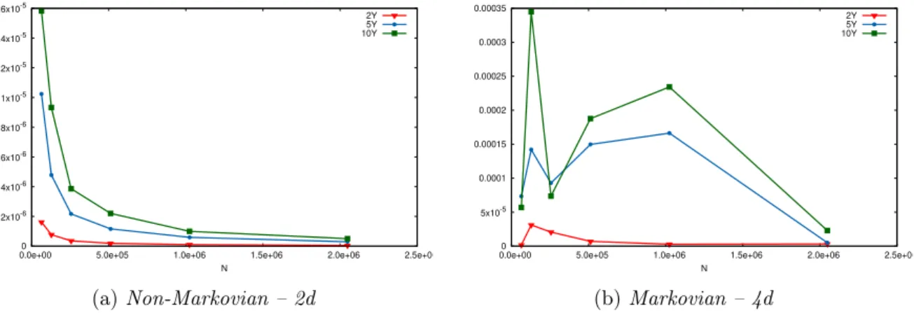
Figure 2
Indeed, let pU, V q a two-dimensional correlated and standard-ized normal distribution with correlation ρ and cumulative distri-bution function (CDF) given by FU,Vρ pu, vq “ PpU ď u, V ď vq. Fast and efficient numerical implementation of such function ex-ists (for example, a C++ implementation of the upper right tail of a correlated bivariate normal distribution can be found in John Burkardt’s website, see [Bur12], which is based on the work of [Don73] and [Owe58]. In our case, we are interested in the com-putation of probabilities of the form
P`U P pu1, u2q, V P pv1, v2q˘. (4.10)
This probability is represented graphically as the integral of the two-dimensional density over the rectangular domain in grey in Figure 2. Now, using FU,Vρ pu, vq, the probability (4.10) is given by
P`U P pu1, u2q, V P pv1, v2q
˘
“ FU,Vρ pu2, v2q ´ FU,Vρ pu1, v2q ´ FU,Vρ pu2, v1q ` FU,Vρ pu1, v1q.
(4.11) This remark will allow us to reduce drastically the computation time induced by the evalua-tion of the condievalua-tional probabilities and so, of the condievalua-tional expectaevalua-tions.
Now, going back to our problem, the QBDPP in the non-Markovian case rewrites (3.25) $ ’ & ’ % p vn`xni1, y n i2 ˘ “ hn`xni1, y n i2˘, 1 ď i1ď N X n , 1 ď i2 ď NnY, p vk`xki1, y k i2 ˘ “ max ˆ hk`xki1, y k i2˘, ÿ j1,j2 π(nm),ki,j pvk`1`x k`1 j1 , y k`1 j2 ˘ ˙ . (4.12)
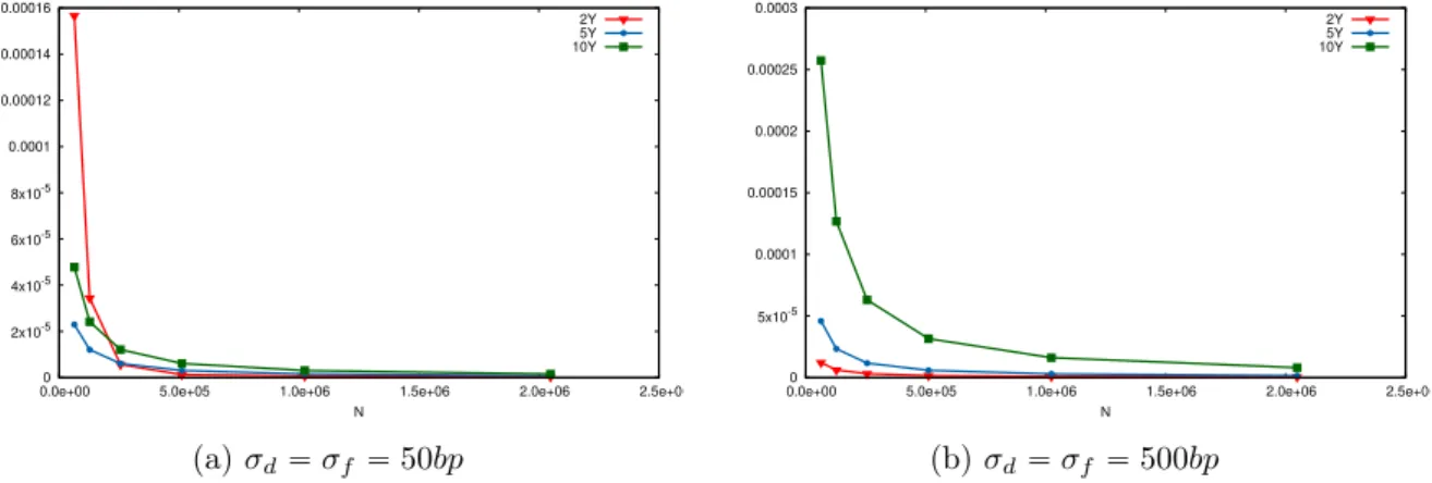
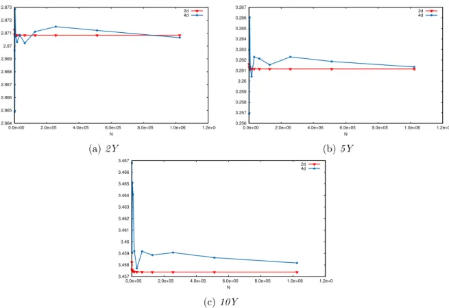
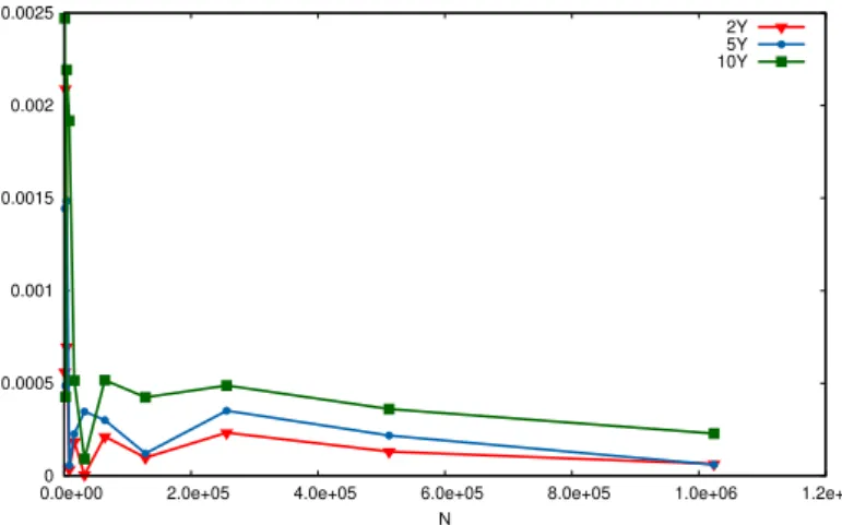
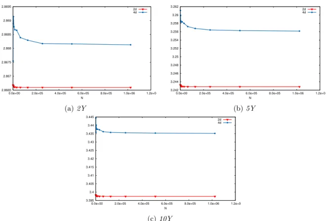
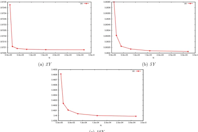
In order to test numerically the two methods, we will evaluate PRDC European and Bermu-dan options with maturities 2Y , 5Y and 10Y . We describe below the market and products parameters we consider. The volatilities of the domestic and the foreign interest rates are not detailed below because we investigate the behaviour of the methods with respect to σdand σf.