HAL Id: hal-00296560
https://hal.archives-ouvertes.fr/hal-00296560
Submitted on 29 May 2008
HAL is a multi-disciplinary open access
archive for the deposit and dissemination of
sci-entific research documents, whether they are
pub-lished or not. The documents may come from
teaching and research institutions in France or
abroad, or from public or private research centers.
L’archive ouverte pluridisciplinaire HAL, est
destinée au dépôt et à la diffusion de documents
scientifiques de niveau recherche, publiés ou non,
émanant des établissements d’enseignement et de
recherche français ou étrangers, des laboratoires
publics ou privés.
radon measurements: sensitivity to cumulus convection
parameterization
K. Zhang, H. Wan, M. Zhang, Biao Wang
To cite this version:
K. Zhang, H. Wan, M. Zhang, Biao Wang. Evaluation of the atmospheric transport in a GCM using
radon measurements: sensitivity to cumulus convection parameterization. Atmospheric Chemistry
and Physics, European Geosciences Union, 2008, 8 (10), pp.2811-2832. �hal-00296560�
© Author(s) 2008. This work is distributed under the Creative Commons Attribution 3.0 License.
Chemistry
and Physics
Evaluation of the atmospheric transport in a GCM using radon
measurements: sensitivity to cumulus convection parameterization
K. Zhang1,4, H. Wan2, M. Zhang3, and B. Wang11LASG, Institute of Atmospheric Physics, Chinese Academy of Sciences, Beijing, China 2International Max Planck Research School on Earth System Modelling, Hamburg, Germany 3LAPC, Institute of Atmospheric Physics, Chinese Academy of Sciences, Beijing, China 4Graduate School of the Chinese Academy of Sciences, Beijing, China
Received: 29 November 2007 – Published in Atmos. Chem. Phys. Discuss.: 5 February 2008 Revised: 15 April 2008 – Accepted: 10 May 2008 – Published: 29 May 2008
Abstract. The radioactive species radon (222Rn) has long been used as a test tracer for the numerical simulation of large scale transport processes. In this study, radon trans-port experiments are carried out using an atmospheric GCM with a finite-difference dynamical core, the van Leer type FFSL advection algorithm, and two state-of-the-art cumulus convection parameterization schemes. Measurements of sur-face concentration and vertical distribution of radon collected from the literature are used as references in model evaluation. The simulated radon concentrations using both convection schemes turn out to be consistent with earlier studies with many other models. Comparison with measurements indi-cates that at the locations where significant seasonal varia-tions are observed in reality, the model can reproduce both the monthly mean surface radon concentration and the annual cycle quite well. At those sites where the seasonal variation is not large, the model is able to give a correct magnitude of the annual mean. In East Asia, where radon simulations are rarely reported in the literature, detailed analysis shows that our results compare reasonably well with the observations.
The most evident changes caused by the use of a differ-ent convection scheme are found in the vertical distribution of the tracer. The scheme associated with weaker upward transport gives higher radon concentration up to about 6 km above the surface, and lower values in higher altitudes. In the lower part of the atmosphere results from this scheme does not agree as well with the measurements as the other scheme. Differences from 6 km to the model top are even larger, al-though we are not yet able to tell which simulation is better due to the lack of observations at such high altitudes.
Correspondence to: K. Zhang
1 Introduction
The interaction between atmospheric chemistry and climate change has been a hot topic in recent years in climate re-search and environmental sciences. Both chemical transport models (CTMs) and general circulation models (GCMs) have been used to address this issue. Typically, a large number of chemical species, either inert or reactive, are involved. A realistic simulation of the distribution, lifetime and climate effects of these species relies on sound information about the emissions, good knowledge of the transformation mech-anisms, and reliable representation of the atmospheric trans-port, the last of which is the focus of this paper. The most important transport processes in a numerical model include large scale advection, cumulus convection and vertical diffu-sion. These processes redistribute the chemical species at a global scale and provide background concentrations for the chemical reactions and the subsequent processes happening in the climate system. Therefore a detailed validation of the transport processes is an indispensable step before a model is put into any practical application.
Radon (222Rn) has long been used as tracer in studies of atmospheric transport. As a noble gas and the radioactive decay product of radium (226Ra), it exists in most types of rock and soil, and is emitted from ice-free land surface with a rather uniform rate. It has a half-life time of 3.82 days – similar to some important reactive chemicals, e.g. SO2 –
but is removed from the atmosphere only by radioactive de-cay. The relatively simple life cycle renders radon a suitable indicator for transport tests. Meanwhile, measurements of atmospheric radon concentration available from distributed observatories provide a good reference for model evaluation. In the 1990’s, two coordinated model intercomparisons of radon transport simulations were carried out, which pro-vided an overview of the models’ performance although the
observations available at that time were quite limited (Jacob et al., 1997; Rasch et al., 2000). A number of publications reported on evaluation studies for individual transport mod-els (Mahowald et al. 1997; Dentener et al. 1999; Considine et al. 2005, among others). In addition, radon has been used as an indicator to investigate other issues. For example, Fe-ichter and Crutzen (1990) evaluated a convective transport scheme designed for a CTM driven by monthly mean cli-matology; Mahowald et al. (1995) compared seven cumulus convection parameterizations in a one-dimensional column model through comparison of the simulated radon profiles. Olivi´e et al. (2004) tested four different sets of vertical diffu-sion coefficients in the TM3 chemical transport model. The work by Genthon and Armengaud (1995) was the first one in the literature using radon to test and compare the tracer transport processes in GCMs.
In this study, radon transport experiment is carried out with the Gridpoint Atmospheric Model of IAP-LASG (GAMIL) developed in the State Key Laboratory of Numerical Mod-eling for Atmospheric Sciences and Geopgysical Fluid Dy-namics (LASG) at the Institute of Atmospheric Physics (IAP) of the Chinese Academy of Sciences.
The overall ability of this global model to represent the mass distribution of radon and its seasonal variability is ex-amined. The work presented here differs from previous stud-ies in three major aspects: first, a new general circulation model with some unique features is used; second, we are par-ticularly interested in the comparison between two state-of-the-art cumulus convection parameterization schemes. Last but not least, the validation data in this work include not only the frequently cited observations obtained before 1990, but also new measurements published in recent years (see Sect. 3).
So far CTMs have been used extensively in atmospheric chemistry studies. However, independency between the ex-ternal meteorological data and the transport scheme within a transport model sometimes leads to significant errors. This problem can eventually be solved in GCMs if the Navier-Stokes equations and the tracer mass budget are discretized in a consistent way. As for the feedback of chemistry-related processes to atmospheric circulation and its impact on future climate change, the instantaneous interactions in GCMs are certainly advantageous.
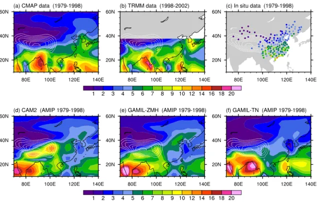
GAMIL is a global atmospheric GCM with a finite differ-ence dynamical core. Most of the physics parameterizations come from the National Center for Atmospheric Research (NCAR) Community Atmosphere Model version 2 (CAM2, Collins et al., 2003) which is a spectral transform model. Although sharing most parts of the physics package makes GAMIL similar to CAM2 in many aspects of the model cli-mate, distinctions due to differences between the dynamical cores are still clearly detectable. The GAMIL model appears to have its particular merits in simulating the Asian mon-soon circulation (Wan et al., 2006; Yang et al., 2007). As an example, we present in Fig. 1 summer precipitation in East
Asia, where severe problems in the Himalaya/Tibetan region in many other models (see, e.g., Fig. 1d here and Fig. 2 in Tost et al. 2006) are evidently reduced (Fig. 1e, f) in GAMIL. So far the GAMIL model has been used in atmosphere-alone applications such as AMIP (Atmospheric Model Intercom-parison Project1) and SMIP (Seasonal Prediction Model In-tercomparison Project2) experiments (Wan et al., 2006; Yang et al., 2007; Shi et al., 2008). It is also the atmosphere com-ponent of the Flexible Global Ocean-Atmosphere-Land Sys-tem (FGOALS, Yu et al., 2008) which has been used in the IPCC AR4 experiments (see, e.g., van Ulden and van Olden-borgh, 2006; Yu et al., 2008). Currently an aerosol module is under development for GAMIL, from which arises the moti-vation for transport validation.
Cumulus convection has a profound impact on the hy-drological cycle of the climate system, the dynamics of the atmospheric circulation, and the mass budget of chemical species. It is also one of the major sources of uncertainty in climate simulations. In the past decades, a number of schemes have been proposed to parameterize this process in large scale atmospheric GCMs (see Arakawa 2004 for a re-view), among which the most widely used in recent years are probably the schemes by Tiedtke (1989) and Zhang and Mc-Farlane (1995). For example, CAM2 and MATCH (Rasch et al., 1997) utilize the Zhang-McFarlane scheme combined with Hack’s proposal (1994) (hereafter ZMH); ECHAM4 and 5 (Roeckner et al., 1996, 2003, 2006) employ the Tiedtke scheme with further modifications by Nordeng (1994) (here-after TN). The algorithm in the ECMWF operational model IFS is also a further development of the Tiedtke (1989) scheme (Bechtold et al., 2004). The ZMH and TN schemes both take the mass-flux form, but have differences in the clo-sure method, triggering conditions for convection and for-mulations for precipitations. Summaries of the details can be found in Sect. 2b of Liu et al. (2005) and Table 1 of Tost et al. (2006). After a lot of comparison studies with various mod-els, it has been found that both schemes have strengths and weaknesses, and the actual performance is model-dependent. Interestingly, we saw Liu et al. (2005) applying the TN scheme from ECHAM4 to CAM2, and later Tost et al. (2006) implementing the ZMH scheme in ECHAM5.
The GAMIL model also has these two convection schemes in its physics package. In the AMIP simulations the TN scheme leads to a significantly improved rainfall simulation in the Indian and East Asia monsoon regions, in terms of both spatial distribution and temporal variation (Fig. 1; Wan et al., 2006). On the other hand, due to the resulting changes in water vapor and cloud distribution, the top-of-atmosphere (TOA) energy balance is violated, indicating necessity of fur-ther tuning. As for the impact on tracer transport, no com-parison has been done for the GAMIL model before this work. There have been publications investigating impact of
1http://www-pcmdi.llnl.gov/projects/amip/index.php 2http://grads.iges.org/ellfb/SMIP2/smip2.top.html
Fig. 1. Observed and simulated summer precipitation (June-July-August average, unit: mm day−1) in East Asia: (a) the CPC Merged
Analysis of Precipitation (CMAP, http://www.cdc.noaa.gov/cdc/data.cmap.html); (b) the Tropical Rainfall Merged Mission (TRMM,http:// trmm.gsfc.nasa.gov/trmm rain/Events/trmm climatology 3B43.html); (c) in situ measurements at 160 observatories in China; (d) simulation by CAM2; (e) simulation by GAMIL with the Zhang-McFarlane-Hack cumulus convection scheme; (f) simulation by GAMIL with the Tiedtke-Nordeng convection scheme. The plotted CMAP and in situ data are averages over the 1979–1998 period. The TRMM data are the 1998–2002 average obtained from the NCAR AMWG diagnostic package. Model simulations are the 1979–1998 average from AMIP experiments. The dashed white contours indicate surface topography in the GCMs (from 2000 to 5000 m above sea level, with an interval of 500 m).
convection on radon transport, but using other parameteriza-tion schemes (Feichter and Crutzen, 1990; Mahowald et al., 1995). As for comparison between ZMH and TN, only the impact on the general circulation has been investigated (e.g., Liu et al., 2005; Song, 2005; Tost et al., 2006). In this study we put our focus on the sensitivity of radon transport.
The rest of the paper is organized as follows: more infor-mation about the model and the experiments is provided in Sect. 2. The radon measurements used as reference are intro-duced in Sect. 3. Section 4 describes the simulated global radon distributions. Comparison of surface concentration with observation is presented in Sect. 5. Analysis of the ver-tical profiles is given in Sect. 6. Section 7 summarizes the study and draws the conclusions.
2 Model and experiments
The prognostic variables of the hydrostatic GAMIL model are the horizontal wind, temperature, surface pressure and the mixing ratio of tracers. The spatial discretization on a C-type latitude-longitude grid originated from the work of Zeng
et al. (1985). A coordinate transformation in the meridional direction was introduced by Wang et al. (2004) to enlarge the zonal grid sizes in the polar regions and thus improve the computational stability. The model version used in this study has 128 longitudes and 60 latitudes. Locations of the grid points between 66◦N and 66◦S are exactly the same as the T42 Gaussian grid. In the vertical, the computational do-main extends from the earth’s surface to 2.194 hPa, unevenly divided into 26 layers in a pressure-based sigma coordinate. Roughly speaking, there are 3 layers in the boundary layer, 14 in the free troposphere, and 9 in the stratosphere. A semi-implicit time stepping scheme conserving the total effective energy was introduced by Wang and Ji (2006). (The origi-nal text was in Chinese. A short summary in English can be found in Zhang et al. 2008.) The large scale advection of wa-ter vapor is handled by the Two-step Shape-Preserving Ad-vection Scheme (TSPAS, Yu 1994). The Flux-Form Semi-Lagrangian (FFSL) transport algorithm proposed by Lin and Rood (1996) has also been introduced into this model (Zhang et al., 2008).
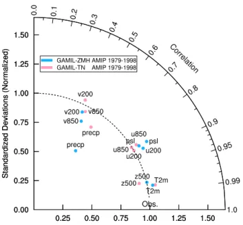
Fig. 2. Taylor diagram showing the space-time variability in AMIP simulations performed with two versions of the GAMIL model using the Zhang-McFarlane-Hack and the Tiedtke-Nordeng con-vection schemes, respectively. The CMAP precipitation data and the NCEP/DOE Reanalysis-II are used as reference (referred to as “Obs.” in the diagram). The statistics are calculated using monthly mean data from January 1979 to December 1998 between 60◦S and
60◦N. The meteorological variables shown include sea level
pres-sure (“psl”), 2-m temperature (“T2m”), precipitation rate (“precp”), 500 hPa geopotential height (“z500”), as well as the zonal and meridional wind at 200 hPa and 850 hPa (labeled as “u200”, “v200”, “u850”, and “v850”, respectively).
As mentioned in the previous section, most of the physics parameterizations are the same as in CAM2, except that the TN convection scheme is also implemented. The bound-ary layer turbulent mixing scheme is an explicit, non-local as described in Holtslag and Boville (1993) and Boville and Bretherton (2003). Other details about the physics package can be found in Collins et al. (2003).
The overall performance of the two versions of GAMIL in general circulation simulation is shown in Fig. 2 with a Taylor diagram (Taylor, 2001). Cosine of the polar angle of a point in the diagram equals the correlation coefficient be-tween simulation and reanalysis; The radial distance from the origin indicates the standard deviation of the simulated field normalized by that of the corresponding reanalysis. The statistics indicated in in Fig. 2 are calculated using monthly mean data between 60◦S and 60◦N in AMIP simulations covering the period from January 1979 to December 1998. Judging from this diagram, the two model versions are of similar quality, except that the variance error of precipitation is significantly reduced in the TN simulation. The correla-tion between model result and the NCEP/DOE Reanalysis-II is about 0.98 for 2-m temperature (labeled as “T2m” in the
diagram) and 0.97 for 500 hPa geopotential height (“z500”); The correlation is around 0.85 for sea level pressure (“psl”), as well as for the zonal wind at the 850 hPa (“u850”) and 200 hPa level (“u200”). Simulations of the meridional wind (“v850” and “v200”) are less accurate. Precipitation rates given by the model (“precp”) are correlated with the CMAP data Xie and Arkin (1997) with a coefficient of about 0.57. The simulated space-time variances are in general in good agreement with the reanalysis, except that the variability in precipitation is underestimated. The performance indicated in Fig. 2 is similar to the AMIP I multi-model ensembles as shown in Fig. 14 in Gates et al. (1999). For further details of the climate simulations with GAMIL, the interested readers are referred to the work by Wan et al. (2006) and Yang et al. (2007).
Apart from the transport processes, emission is also an important factor that determines radon distribution in the atmosphere. Based on measurements of 222Rn concentra-tion and210Pb deposition flux, previous studies have derived estimates of continental radon emission ranging from 0.71 to 1.2 atom cm−2s−1(Turekian et al., 1977; Lambert et al., 1982).
For validation of global models, the emission is generally assumed to be spatially uniform (1 atom cm−2s−1) from ice-free land surfaces, which is believed to be accurate within 25% globally and within a factor of 2 regionally (Jacob et al., 1997). In this study we follow the recommendation of the World Climate Research Program (WCRP) Cambridge Workshop of 1995 (Rasch et al., 2000): The continental emission is set to 1 atom cm−2s−1between 60◦S and 60◦N and 0.5 atom cm−2s−1between 60◦N and 70◦N, except for Greenland. Emission over the oceans and the Antarctica is assumed to be zero.
Some modelling studies have indicated that taking into ac-count the latitudinal and regional gradients of radon emis-sion could lead to a more realistic simulation of the surface concentration, especially at high-latitude sites (e.g. Lee and Feichter, 1995; Guelle et al., 1998; Conen and Robertson, 2002). However, we stick to the WCRP 1995 settings so that there are more information available from other models to which our results can be compared directly.
In this study, we conduct climate simulations using the GAMIL model with radon treated as passive tracer. The sea surface temperature (SST) and sea ice data as bound-ary conditions are the 1979–2001 average without interan-nual variation. The original data at 1◦×1◦ resolution are obtained from the Program for Climate Model Diagnosis and Intercomparison (PCMDI, http://www-pcmdi.llnl.gov/ projects/amip/index.php) and interpolated to the model grid using area-weighted interpolation. Meteorological fields at the initial time step are interpolated from the ERA40 reanal-ysis at 1 January 1979 00:00 UTC. The initial concentration of radon is zero. Two six-year simulations are conducted using the ZMH and TN convection scheme, respectively, of which the first year is discarded as the spin-up phase. All
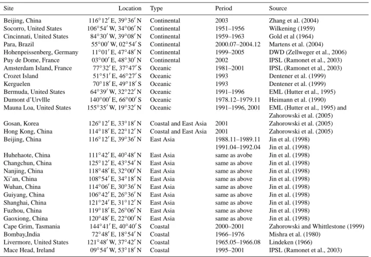
Table 1. Detailed information about the surface radon measurements used in this study. Regarding data source, DWD stands for Deutscher Wetterdienst (German Weather Service); IPSL for Institut Pierre-Simon Laplace; EML for DOE/Environmental Measurements Laboratory. Location of these site are also plotted in Fig. 3 and Fig. 4.
Site Location Type Period Source
Beijing, China 116◦12′E, 39◦36′N Continental 2003 Zhang et al. (2004)
Socorro, United States 106◦54′W, 34◦06′N Continental 1951–1956 Wilkening (1959)
Cincinnati, United States 84◦30′W, 39◦08′N Continental 1959–1963 Gold et al (1964)
Para, Brazil 55◦00′W, 02◦54′S Continental 2000.07–2004.12 Martens et al. (2004)
Hohenpeissenberg, Germany 11◦01′E, 47◦48′N Continental 1999–2005 DWD (Zellweger et al., 2006)
Puy de Dome, France 03◦00′E, 48◦30′N Continental 2002 IPSL (Ramonet et al., 2003)
Amsterdam Island, France 77◦32′E, 37◦47′S Oceanic 1981–2001 IPSL (Ramonet et al., 2003)
Crozet Island 51◦51′E, 46◦27′S Oceanic 1993 Dentener et al. (1999)
Kerguelen 70◦18′E, 49◦18′S Oceanic 1993 Dentener et al. (1999)
Bermuda, United States 64◦39′W, 32◦22′N Oceanic 1991–1996 EML (Hutter et al., 1995)
Dumont d’Urvllle 140◦00′E, 66◦00′S Oceanic 1978.12–1979.11 Heimann et al. (1990)
Mauna Loa, United States 155◦35′W, 19◦32′N Oceanic 1991–1996, 2001 EML (Hutter et al., 1995) and
Zahorowski et al. (2005) Gosan, Korea 126◦12′E, 33◦18′N Coastal and East Asia 2001 Zahorowski et al. (2005)
Hong Kong, China 114◦18′E, 22◦12′N Coastal and East Asia 2001 Zahorowski et al. (2005)
Beijing, China 116◦12′E, 39◦36′N East Asia 1988.11–1989.11 Jin et al. (1998)
1991.04–1992.04 Jin et al. (1998) Huhehaote, China 111◦42′E, 40◦48′N East Asia same as avobe Jin et al. (1998)
Changchun, China 125◦12′E, 43◦54′N East Asia same as above Jin et al. (1998)
Nanjing, China 118◦48′E, 32◦00′N East Asia same as above Jin et al. (1998)
Xi’an, China 108◦54′E, 34◦18′N East Asia same as above Jin et al. (1998)
Wuhan, China 114◦06′E, 30◦36′N East Asia same as above Jin et al. (1998)
Guiyang, China 106◦42′E, 26◦36′N East Asia same as above Jin et al. (1998)
Shanghai, China 121◦24′E, 31◦12′N East Asia same as above Jin et al. (1998)
Fuzhou, China 119◦18′E, 26◦06′N East Asia same as above Jin et al. (1998)
Gaoxiong, China 120◦48′E, 22◦00′N East Asia same as above Jin et al. (1998)
Cape Grim, Tasmania 144◦41′E, 40◦40′S Coastal 2000–2001 Zahorowski and Whittlestone (1999)
Bombay,India 72◦48′E, 18◦54′N Coastal 1966–1976 Mishra et al. (1980)
Livermore, United States 121◦48′W, 37◦42′N Coastal 1965.05–1966.08 Lindeken (1966)
Mace Head, Ireland 09◦54′W, 53◦18′N Coastal 1995–2001 IPSL (Ramonet et al., 2003)
the diagnostics presented in this study are based on the 6-h output of the last five years.
It is worth noting that in our experiments the large scale advection of radon is handled by the van Leer type FFSL scheme. In an earlier study (Zhang et al., 2008) it has been found that when the TSPAS scheme is used, significant bi-ases occur in idealized test cbi-ases and in the radon transport simulations, especially in the polar regions and in the up-per part of the atmosphere. In contrast, the FFSL scheme produces much more reasonable results. A natural decision following that work may be to replace the old scheme by FFSL for all tracers in the model. However, the complicated feedback of water vapor to the atmospheric general circula-tion will probably lead to some changes in the climate state as well (Rasch and Kristjansson, 1998). So far in all the other applications of the GAMIL model the TSPAS advec-tion scheme have been used. Given that radon is a passive tracer in this study, we use TSPAS for water vapor and FFSL for radon, so that the GCM employed here is exactly the same as its “IPCC version”.
3 Radon measurements
This section briefly introduces the observational data used for comparison with the model simulations. The measurements are of two types: radon concentration near the earth’s surface and the vertical profiles.
3.1 Surface concentration
Surface radon concentration at 27 sites worldwide are col-lected from the literature for use here. Basic information about these measurements is presented in Table 1, Fig. 3 and Fig. 4. At 18 sites monthly mean concentration is available. Since some of these monthly means are calculated from mea-surements at higher frequencies (e.g. hourly or 6-h data), the standard deviation of all the samples within the same month are also calculated and plotted. For the other 9 sites and Bei-jing which are city stations in China, the annual mean has been reported by Jin et al. (1998).
It should be pointed out that the heights and measuring methods differ significantly from site to site. The details will
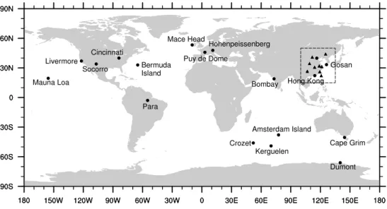
Fig. 3. Locations of the surface radon measurements used in this study. Dots indicate the sites where monthly data are available. Triangles denote the sites where only the annual mean has been reported. The area in the dashed frame is enlarged in Fig. 4.
Fig. 4. Locations of the surface radon concentration measurements in East Asia. Dots indicate the sites where monthly data are avail-able. Triangles denote the sites where only the annual mean has been reported. Gray crosses on the map indicate grid points in the GCM. The dashed lines are the boundary of grid cells.
be mentioned in the following sections during the analysis. For a complete description of the measurements, the readers are referred to the publications listed in Table 1.
Another important fact to note is that not all the sites listed in Table 1 have multi-year continuous observations. It
is well-known that the interannual variability of the atmo-spheric general circulation is high. The same must be true for radon concentration at specific locations. However, radon observation is quite limited; Moreover, our simulations pro-ceed only six years and the SST and sea ice forcing is re-peated from year to year. It is therefore impossible to rea-sonably estimate the uncertainty associated with interannual variation from either the measurements or our experiments. During the discussion on model evaluation in the following sections we have to take this into account and bear in mind that the monthly means observed in a specific year at a spe-cific station may deviate significantly from the long-term cli-matology.
3.2 Vertical profiles
Observations of the vertical distribution of radon are rare. Summer and winter profiles of the Northern Hemisphere have been compiled by Liu et al. (1984), who computed the average of individual measurements at different continental locations from 1950 to 1972. The winter profile is the aver-age of 7 sites and the summer profile 23 sites. Although the data are relatively old, they are quite often cited in related studies.
Kritz et al. (1998) presented a group of free tropospheric radon profiles measured by aeroplane in the summer of 1994 from the earth’s surface till 11.5 km altitude. The start-ing measurstart-ing place was Moffett Field (37.4◦N,122.0◦W) in California, USA. 11 profiles were obtained from June to August 1994. We use the average of the 7 profiles in June to compare with our five-year-mean simulation in the same month. In contrast to Liu et al. (1984), this set of data pro-vide information about radon distribution over the offshore
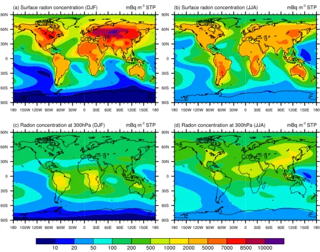
Fig. 5. Geographical distribution of radon concentration simulated with GAMIL using the Zhang-McFarlane-Hack convection scheme. The top panels are results on the lowest model level (σ =0.9925); The bottom panels are at 300 hPa. The left (right) column shows the DJF (JJA) average of monthly mean.
regions. A similar data set published by Zaucker et al. (1996) was compiled from 9 flights in August 1993 from cities Nova Scotia and New Brunswick on the east coast of Canada to the western North Atlantic Ocean during the North Atlantic Re-gional Experiment (NARE) Intensive. These measurements covered the vertical range from surface to about 5.5 km.
4 Simulated global distribution
Before comparison with in situ observations, we first give an overview of the model’s performance by presenting the ge-ographical distribution of the simulated radon concentration on the lowest model level (σ =0.9925) and at 300 hPa, as well as the zonally averaged pressure-latitude cross sections. 4.1 Geographical distribution
The December-January-February (DJF) and June-July-August (JJA) mean surface radon concentrations simulated with the ZMH convection scheme are shown in Fig. 5a and 5b, respectively. Here we use the same unit as the
measurements, i.e. millibequerel per standard cubic me-ter at 273.15 K and 1013.25 hPa (mBq m−3 STP). In this simulation, the highest values appear over the continents, with magnitude of about 104mBq m−3 STP in DJF and 6×10³mBq m−3STP in JJA. Radon concentration over the ocean is much lower (101–103mBq m−3 STP) due to the absence of emission there. Since the atmospheric stabil-ity is generally much higher in winter than in summer, the suppressed upward transport leads to winter concentrations about a factor of 2 to 3 higher than the summer values.
Results at the 300 hPa level are shown in the bottom panels of Fig. 5. High concentrations appear over south America and south Africa due to the deep low-pressure systems in these regions and the associated strong updraft. The large area of high concentration over Asia in JJA is clearly related to the Asian summer monsoon. The largest values exceed 103mBq m−3STP.
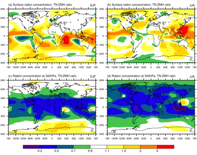
Changes in the convection parameterization cause evident differences in the radon concentration. Near the earth’s sur-face, values in the convection regions in the TN run are more than 30% larger than ZMH (Fig. 6a, b). At 300 hPa, the
Fig. 6. Differences in the simulated radon concentration between the TN and ZMH simulations. The plotted quantity is the the TN:ZMH ratio. (a) and (b): on the lowest model level (σ =0.9925); (c) and (d): at 300 hPa.
TN scheme generally produces significantly lower concen-trations in the middle and low latitudes (Fig. 6c, d).
4.2 Zonal mean
The pressure-latitude cross sections of the zonal mean radon concentration in the ZMH simulation are shown in the top panels of Fig. 7. Here we change the unit to volume mixing ratio (10−21mol mol−1) so as to facilitate direct comparison with other publications.
In boreal winter (Fig. 7a), the highest concentrations are located in the northern mid-latitudes and near the earth’s sur-face due to the emission and the atmospheric stability. The lowest values occur over the Antarctica and near model top. In this season the most active convection motions are in the Southern Hemisphere, especially in the South Pacific Con-vergence Zone (SPCZ). The convective transport leads to a high-concentration region between the equator and 30◦S throughout the troposphere. From 30◦S southwards, the centration decreases very fast on all vertical levels. The con-tours are almost perpendicular to the earth’s surface.
In boreal summer, the strongest convective pumping ap-pears in the Northern Hemisphere. The highest radon con-centrations in the upper troposphere shift accordingly to around 25◦N (Fig. 7b). It should be pointed out that in Fig. 7, no extrapolation was done in remapping the concentration from model grid to pressure levels. This led to missing values on, for example, the 1000 hPa level over land in the tropics. When the zonal mean was calculated, these missing values were ignored and the zonal average represents mainly results over the oceans on the specific level at the specific latitude. This is the reason why we see relatively low concentrations between 30◦S and 30◦N below 900 hPa in panel b and c of Fig. 7. We have also tried doing the calculation with extrap-olation, and got increasing concentration towards the surface in the aforementioned areas which was similar to published results from other models.
Figure 7d, e and f are the differences between experiments TN and ZMH as expressed by the ratio of the zonal mean radon concentration in these experiments. It is clear that in the convection-active regions, the concentration is higher in the lower atmosphere and lower in the upper levels in the
Fig. 7. (a–c): Zonally averaged DJF, JJA and annual mean radon concentration simulated by GAMIL using the ZMH convection scheme. (d–f): Differences between the TN simulation and the ZMH run as indicated by the TN:ZMH ratio.
TN simulation. The largest difference exceeds a factor of 2. This may possibly be attributed to the fact that the mean upward mass flux in the TN simulation is weaker than in ZMH. Figure 8 shows the cumulus convection mass flux in the two simulations. The original model output on sigma levels are plotted so as to avoid possible artifacts produced by interpolation. Note that the ZMH scheme has two com-ponents: the Zhang and McFarlane (1995) parameterization (hereafter ZM95) for penetrative convection, and the Hack (1994) scheme (hereafter Hack94) for the shallow and mid-dle tropospheric convection. The corresponding subroutines in the model are called successively and both contribute to tracer transport. The TN scheme handles all three types of convective activities, but only allows one type to take place each time the scheme is activated. The deep convection mass flux given by the ZM95 scheme (Fig. 8g–i) is similar to the total flux in the TN simulation (Fig. 8d–f), both in magni-tude and in the characteristic pattern. A feature worth noting is that in the TN run the strongest updraft in the tropics ap-pears between 600 and 800 hPa and decreases fast in the near surface levels. In contrast, the strong updraft (>4 g m−2s−1) given by the ZM95 scheme extends to the surface. The
ver-tical motion resulting from the Hack94 parameterization is characterized by strongest ascending in the near-surface lev-els over the storm tracks, as well as secondary strong mo-tions in the upper troposphere and tropical lower atmosphere. The comprehensive effect is that the total mass flux given by ZMH is significantly larger, especially at the model lowest levels.3Given that the source of radon resides at the surface, this implies considerably more effective convective pumping towards the higher altitudes in the ZMH simulation.
In the work by Considine et al. (2005), radon transport tests were conducted with and without convective processes in a chemical transport model. The contribution of convec-tive transport to the zonal and annual mean radon distribution was illustrated in their Fig. 12, which showed by and large
3The dramatic difference between the two simulations is not a peculiar feature of this specific model. The standard CAM (using the ZMH scheme) also shows relatively strong updraft in the up-per troposphere, although not as prominent as here; As for the TN parameterization, convective mass flux similar to the lower panels in Fig. 8 has been observed in previous studies when the Tiedtke scheme was implemented in the CAM model (X.-L. Song, 2008, personal communication).
Fig. 8. Zonally averaged DJF, JJA and annual mean net convective mass flux (unit: g m−2s−1). The first and second rows are the total
convective mass flux simulated with the Zhang-McFarlane-Hack (ZMH) parameterization scheme and the Tiedtke-Nordeng (TN) scheme, respectively. The third row shows the contribution from deep convection in the ZMH simulation. The last row shows the mass flux associated with the middle and shallow convection in the ZMH simulaiton.
the same pattern as in Fig. 7f here. Note that in their control experiments, the convection-related variables (vertical mass flux, entrainment and detrainment rates) were taken from the meteorological data driving the CTM, therefore their esti-mate was in fact the direct effect of convection on radon distribution. In our GCM, change of convection scheme also affects the transport process by indirectly modifying the general circulation. However, similarity between our results and theirs confirms that the differences we see in Fig. 7 are mainly due to the direct effect of convective transport. 4.3 Comparison with other models
Results of the radon transport test from many other models are available in the literature. Figure 5 and 7 here can be compared with, e.g., Figs. 5 and 6 in Jacob et al. (1997), Figs. 1 and 2 in Dentener et al. (1999) and Fig. 5 in Reith-meier and Sausen (2002). From the intercomparison, it is clear that the two versions of the GAMIL model with differ-ent convection parameterizations both behave reasonably in large scale transport of passive tracer. The differences de-tected above are well within the range of inter-model dis-crepancies. Thus we can not yet conclude which version is better. In the next section radon concentration measurements are used for more detailed comparison.
5 Comparison with surface measurements
In order to evaluate the simulated surface radon concentra-tion with respect to in situ measurements, model output is lin-early interpolated to the location of the observations. Com-parison of the monthly mean concentration at 18 sites is sum-marized in Fig. 9, which shows a good agreement on the whole. Taking all months at all the 18 sites into account (Fig. 9a), the correlation coefficient between simulation and observation is 0.87 (0.85) in the ZMH (TN) run. Out of a total of 213 samples (12×18, three samples missing, see Figs. 10f and 13f), 78.7% (74.1%) in the ZMH (TN) experi-ment agree within a factor of 2 with the measureexperi-ments. Re-sults in summer and in winter (Fig. 9b, c) are of similar qual-ity. Regarding different types of sites (Fig. 9d–f), it can be clearly seen that locations over the oceans (i.e. the remote is-lands) are characterized by much lower concentrations than the other sites. In panel (e) a cluster of points with measured concentration around 6×10²mBq m−3STP indicates slight overestimate in both simulations. These points are in fact from a single site (Mace Head), for which detailed discus-sions are deferred till later.
From Fig. 9 it is difficult to tell any concrete difference between results obtained with different convection schemes. In the following subsections we take a closer look at the monthly mean results at each single location. The continen-tal, oceanic and costal sites are analyzed separately.
5.1 Continental sites
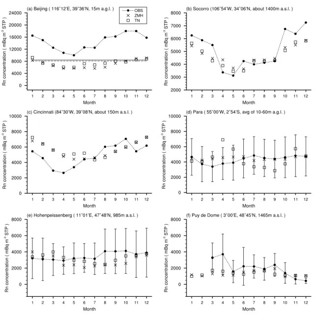
The simulated and observed monthly mean radon concentra-tions at six continental sites are shown in Fig. 10. Variance of the observations within a month is also indicated in the figure when the information is available.
The continental sites are characterized by high surface concentrations of 103–104mBq m−3STP. For Fig. 10a (Bei-jing, 116◦12′E, 39◦36′N) we need to point out that the monthly mean indicated by full circles was measured on the fourth floor of a building (15 m above the ground), which has been found to have a much higher annual mean than other observations. The merit of this data set is that it shows the seasonal variation. When it is used for model validation, a potential systematic difference due to the coarse resolution of our global GCM needs to be taken into account. The an-nual mean reported by Jin et al. (1998) at another location in Beijing (indicated by the solid line in Fig. 10a) and the average of 15 sites in the same city given in Cheng et al. (2002) (the dashed straight line in Fig. 10a) are possibly bet-ter references for the annual mean in a global model. With these facts in mind, we can say that the simulations at Beijing agree well with the reality in both the annual mean and the seasonal variation. The two runs with different convection schemes are almost identical, except for slightly higher con-centration given by the TN scheme in the summer/autumn months (June to September). The concentration at Socorro (106◦54′W, 34◦06′N, Fig. 10b) shows features similar to Beijing. At these mid-latitude locations, the GCM is able to capture the strong seasonal contrast in wind direction and the changes in boundary layer depth. The simulations are therefore quite good.
Cincinnati (84◦30′W, 39◦08′N) is also a mid-latitude site but located within a climatic transition zone between the hu-mid subtropical climate and the huhu-mid continental climate. Radon concentrations are clearly overestimated in winter and spring in both simulations (Fig. 10c). The same problem has been reported by Reithmeier and Sausen (2002) (see the bottom left panel of Fig. 7 therein), who attributed the dis-crepancy to the simplified radon emission in the experiment (i.e. the constant emission rate over land). Their explana-tion was that frost and snow cover in winter and increased soil moisture in spring could reduce the emission flux. Apart from this, negative temperature biases in boreal winter in the GAMIL model over central and northern part of USA and the overly stable boundary layer can also be a reason for the simulated high concentration.
Observations at station Para (55◦W, 2◦54′S, Fig. 10d) are obtained in the Tapajos National Forest in the northern part of Brazil. Martens et al. (2004) reported radon data collected on a tower in this region including measurements within and above the forest canopy (ranging from 0.3 m to 61 m above the ground level). Since radon concentration within the canopy is quite high due to lack of turbulent mixing and the canopy layer is not resolvable in our model, average
Fig. 9. Scatter plot of the simulated and measured monthly mean surface radon concentration of (a) all samples at all the 18 sites, (b) summer samples (JJA in the Northern Hemisphere, DJF in the Southern Hemisphere) at all the 18 sites, (c) winter samples (DJF in the Northern Hemisphere, JJA in the Southern Hemisphere) at all the 18 sites, (d) all samples at 6 remote island sites, (e) all samples at 6 coastal sites, and (f) all samples at 6 continental sites. Results obtained using the ZMH and TN convection scheme are indicated by open circles and crosses, respectively. The dashed lines indicate the range within a factor of 2 of the measurements. Also shown in each panel are the percentage of samples within this range (the P2 values) and the correlation coefficients between simulation and observation (the CR values).
Fig. 10. Observed and simulated monthly mean surface radon concentration at six continental sites. Bars associated with measurements in some panels indicate variance of all the samples (e.g. hourly or 6-h data) within each month. The solid and dashed lines in panel (a) indicate two additional measurements of the annual mean. The abbreviation “a.g.l.” in the titles stands for “above ground level”; “a.s.l.” stands for “above sea level”.
concentration at four altitudes above the 30 m level (32.0 m, 37.0 m, 47.2 m and 61.0 m) are used in this study. Para sta-tion has a typical tropical rainforest climate characterized by small variations in the atmospheric state throughout the year. Consequently the observed monthly mean radon concentra-tion shows much smaller fluctuaconcentra-tions compared to the vari-ance calculated from hourly data in each month (Fig. 10d). The ZMH simulation agrees with the observation well except for slight positive biases in March, April and May. The TN simulation also gives a correct value of annual mean, but pro-duces a spurious peak in April and a trough around Septem-ber. Our analysis reveals that the peak is caused by the
signif-icantly weaker convective mass flux in the rainy season near the earth’s surface at this location (not shown), which is asso-ciated with weaker upward transport from the vicinity of the source. The spurious trough from June to October is caused by the easterly wind bias (Fig. 11) which brings too much fresh air from the Atlantic Ocean and dilutes the radon-rich air over land.
Hohenpeissenberg in Germany (Fig. 10e) is a challenging site for GCMs to simulate because of the orography. The measurements are collected on an isolated mountain rising about 300 m above the surrounding area. At this type of sites, the surface radon concentration depends strongly on
Fig. 11. Monthly mean near-surface wind at Para station simulated with the ZMH convection scheme (top row) and the differences be-tween the TN and ZMH experiments (bottom row).
the status of the boundary layer. In winter and during the night, the boundary layer is usually shallow and the station may possibly level the free atmosphere in the surrounding areas. In case the horizontal wind is weak, radon concen-tration at the station is mainly affected by the local emission and high values will be recorded; When strong wind comes from the neighboring free atmosphere, horizontal transport will lower the local concentration significantly. In summer and during the day when the atmosphere is relatively unsta-ble, vertical transport to higher altitude is strong, resulting moderate local concentrations. Consequently observations at this kind of stations are typically characterized by small sea-sonal variation, as we can see in Fig. 10e. However, the fine orographical feature at Hohenpeissenberg is not resolvable at all in a GCM with approximately 300 km horizontal resolu-tion. Given this fact, results at this site can be regarded as quantitatively correct in the sense of a similar level of sea-sonal variation and the small bias in the annual mean.
Puy de Dome is also difficult to simulate because it is lo-cated on the second highest peak of the Auvergne Moun-tains. For this station, only ten months of data in a single year (March to December 2002) are available (Fig. 10f). Our sim-ulations show a tendency of negative bias on the whole. This may be due to the fact that orography in the model is much smoother than reality, and the location of the site (1465 m above sea level) is therefore farther from the source at sur-face in the numerical model .
5.2 Oceanic sites
Comparison between the observations and simulations on remote islands are presented in Fig. 12. (Station Dumont d’Urville on the coast of Antarctica is also sorted in this group because our experiments assume no emission from Antarctica.) Since these oceanic sites are mainly affected by large scale transport instead of immediate emission and local circulation, a better simulation of the seasonal cycle is expected, which is indeed the case in our results.
Amsterdam Island (77◦32′E, 37◦47′S) in the South In-dian Ocean is a location for monitoring the background radon concentration. Measurements have been obtained as part of the French Trace Gas Monitoring Program (RAMCES) co-ordinated by the Laboratory of Sciences of the Climate and the Environment of the Institut Pierre-Simon Laplace (IPSL) (Ramonet et al., 2003). Used in this study is a data set of 20 years (1981, 1983–2001; No measurement available in 1982). The observed maximum and minimum of monthly means are about 60 mBq m−3STP and 20 mBq m−3STP, re-spectively (Fig. 12a). Records show that during radonic storms, instantaneous concentration can reach 400 mBq m−3STP and in some years even 700 mBq m−3STP (Ra-monet et al., 2003), implying considerable interannual vari-ability. Considering that our experiments are driven by cli-matological SST and proceed only five years, the ZMH sim-ulation in fact agrees well with the observation.
Crozet (51◦51′E, 46◦27′S) and Kerguelen (70◦18′E, 49◦18′S) are also located in the South Indian Ocean but at higher latitudes and lie in the storm track. The validation data in Fig. 12b, c are measurements in the year 1993 from Den-tener et al. (1999). Both the ZMH and TN simulations can reproduce the one-cycle-per-year feature at these sites with highest concentration in winter months. However, overesti-mation is easily detectable. Since there is no local emission, the bias can only be attributed to long range transport. At these sites, wind blows almost continuously from the west throughout the year. The 6-h model output indicates that radon-rich air mass reaching Crozet and Kerguelen originates mainly from the southern part of South America and Africa, which is consistent with earlier studies of Heimann et al. (1990), Mahowald et al. (1997) and Dentener et al. (1999). Dentener et al. (1999) pointed out that positive bias in radon emission over South America in the winter months due to treating frozen soil as non-frozen might be the reason for the aforementioned error at Crozet and Kerguelen. Therefore bi-ases at these two sites should not be considered as defect of numerical models but limitations in the experimental design. As for the effect of different convection schemes, the three site discussed above exhibit a similar feature: radon concen-tration in May to July in the TN simulation is higher than ZMH. The discrepancy is especially large at Amsterdam Is-land. Recall that the most substantial differences in climate state cause by changes in the convection scheme appear dur-ing the summer monsoon months over India, East China and the West Pacific. Since the Asian-Australian monsoon is a planet scale phenomenon, circulation in the South Indian Ocean is inevitably affected. We have looked into the sur-face wind difference and seen that in the TN simulation there is northwest wind anomaly towards these islands from south-east Africa (not shown). Similar anomalies also exist in De-cember and January for Amsterdam Island, although not as significant for the other two sites. The resulting differences in horizontal transport explains the different radon concen-trations in the two simulations.
Fig. 12. As in Fig. 10 but for the remote island (i.e. oceanic) sites.
Figure 12d shows the results at Bermuda islands (64◦39′W, 32◦22′N). Both simulations are qualitatively cor-rect in terms of the order of magnitude, but show some dis-crepancies in the seasonal variation as compared to obser-vation. From the sea level pressure and surface wind fields it is clear that in summer the Azores high is strong and lo-cated over the subtropical North Atlantic. The air reaching Bermuda comes mainly from the eastern part of the North Atlantic Ocean. Radon concentration at the observatory is therefore low. This feature is well reproduced in our model. However, in winter the Bermuda Islands are strongly affected by the radon-rich air from the North American Continent and the westerly wind is overestimated in the simulations. This
explains the relatively large positive bias from late autumn to spring in Fig. 12d.
Dumont d’Urville (140◦E, 66◦S) is an interesting station at which the simulations have an annual cycle similar to the three sites already discussed in this subsection, but the ob-servation tells exactly an opposite story (Fig. 12e). The posi-tive biases in June to September are not difficult to explain after the discussions about the 3 Southern Ocean stations above, although the major origin of radon is South Amer-ica in this case(not shown). As for the summer months, the observed high concentration may be due to local emission from the ice-free coastal area of Antarctica where a constant zero emission is assumed in the experiments. The case of
Fig. 13. As in Fig. 10 but for the coastal sites.
Mauna Loa (Fig. 12f) is in some sense similar: The Hawaii islands are sufficiently large to produce non-negligible local radon emission in reality, but still too small to be resolved by the GCM. The incorrect source information is responsible for the systematically low concentration at Mauna Loa station. 5.3 Coastal sites and East Asia cities
Figure 13 shows the monthly mean surface radon concen-trations at six coastal sites. In reality these are locations on the coast experiencing systematic changes in wind direction throughout a year; In the numerical model, the grid cells in which the observatories are located are recognized as ocean (i.e. no emission), but there is at least one neighboring cell categorized as land at each site. The measurements were
obtained at the transition between large continents and the oceans, thus a correct annual cycle in radon concentration simulation depends mainly on realistic representation of the seasonal wind change, while exact match in each month also relies on detailed features of the circulation in a relatively small region surrounding the site.
Gosan (126◦12′E, 33◦18′N) and Hong Kong (114◦18′E, 22◦12′N) are typical sites in East Asia, a monsoon region that is not very well handled in many models mainly due to the topography in the west. As can be seen in Fig. 13a and b, seasonal cycle at these two sites are quite realistically repro-duced by the GAMIL model. Additional comparison of the annual mean radon concentration at ten Chinese cities with the measurements reported in Jin et al. (1998) is presented
in Fig. 14. Note that an earlier study by Schery and Wasi-olek (1998) has revealed that South China is characterized by very high emissions in reality (equivalent to 1.5 to more than 2.6 atoms cm−2s−1, see Fig. 5 therein). Furthermore the city Gaoxiong (also known as Kaohsiung) in our experiments is actually an oceanic site without local emission. These facts can explain the considerable underestimate at the last four sites in Fig. 14. That being considered, it is fair to say that Fig. 14 also confirms the model’s relatively good perfor-mance in East Asia.
Results at Cape Grim (144◦41′E, 40◦40′S) are also satis-factory (Fig. 13c), while positive biases occur at Bombay on the Indian Peninsula (Fig. 13d) and Livermore on the west coast of North America (Fig. 13f). The former may result from the westerly wind bias that brings an excess of radon-rich air from the continent (not shown). As for Livermore, the 11-month data with large variance (e.g. in October) seem not yet sufficient for a quantitative comparison.
Positive biases also appear at Mace Head in Ireland as compared to the 7-year-mean observation, which can be at-tributed to the overestimated emission. According to Schery and Wasiolek (1998), West and North Europe are character-ized by relatively low emissions. An additional experiment has be conducted using the ZMH convection scheme, but with the emission decreasing linearly from 1 atom cm−2s−1 at 30◦N to 1 atom cm−2s−1at 70◦N as proposed by Conen and Robertson (2002). The recalculated radon concentra-tions are indicated by open circles in Fig. 13e which show an evident improvement.
Comparing the two convection schemes, differences are not evident at the coastal sites in Fig. 13.At the East China city sites the TN scheme gives a slightly higher annual mean concentration.
6 Comparison of vertical profiles
In this section we attempt to investigate the sensitivity of radon simulation to convection scheme by looking into the vertical structure. Presented in Fig. 15 are the vertical pro-files of radon concentration averaged over different geo-graphic regions. In the tropics (Fig. 15b, e) only the annual means are plotted; In the middle latitudes, winter and sum-mer profiles are given separately.
In contrast to the previous section, distinct differences can be detected between the ZMH and TN simulations. The rel-atively weak updraft associated with the TN scheme leads to higher concentration near the surface but lower values above 3 km. The differences are most evident in the tropical ar-eas and in summer. On the other hand, the two convection schemes also produce many similar features. For example, the concentration decreases the fastest with height near the earth’s surface; it appears to be almost constant despite the increasing altitude from 6 km to the tropopause in the low latitudes and during summer in middle latitudes, indicating
Fig. 14. Observed and simulated annual mean surface radon con-centration in ten Chinese cities.
strong vertical transport by cumulus convection. Consider-able seasonal changes occur in the middle latitudes. Summer concentrations are higher at almost all altitudes over the con-tinents while the reverse is true in the lower atmosphere over the oceans.
The upper panels in Fig. 16 compare the simulations over the mid-latitude land areas in the Northern Hemisphere with the compilation results of Liu et al. (1984). The latter were obtained by averaging measurements over the United States and eastern Ukraine. In summer (Fig. 16a), the nearly log-linear decrease of radon concentration from the surface to 4 km is well captured by both convection schemes. The smaller decrease rate between 4 and 8 km is better repre-sented by the ZMH scheme. In the upper troposphere the again enhanced decrease rate seems to be underestimated by both schemes. The observed winter profile (Fig. 16b) also has the three-sector structure but with even stronger con-trasts. The two simulations show less differences than in summer and a smoother change through vertical levels than the observation. Considering the fact that the winter mea-surements consist of only 7 sites while the model results are computed from all the continental grid points between 30◦N and 60◦N, the discrepancies are acceptable.
For the offshore regions, radon concentration profiles have been reported by Kritz et al. (1998) obtained near Moffett Field in California, USA, and by Zaucker et al. (1996) near the western coast of Canada. Figure 16c compares a com-posite of June 1994 profiles from Kritz et al. (1998) with the five-year-mean model results in June averaged from the two coastal cells where the measurements were collected. The error bars (black line) indicate the standard deviation of the measurements. The log-linear decrease till 4 km and the nearly constant concentration from 4 to 10 km above the sur-face are very well represented by the model with both con-vection schemes. This plot can be compared with Fig. 6 in Considine et al. (2005) where the same measurement was used to validate a CTM driven by three different meteoro-logical data sets. They reported near-surface values which
Fig. 15. Vertical profiles of radon concentration simulated with the ZMH and TN convection schemes. Plotted are the averages over different regions as indicated in the title of each panel.
consistently exceeded observations by a factor of 2 to 3, and attributed the biases to the low resolution (5◦longitudinal) in their study. The horizontal grid in our experiments has only half the grid size (2.8◦). In addition, the cells from which the Moffett Field profile is obtained do not have local emis-sions. These two facts possibly explain the improvement in our simulations.
Figure 16d shows the simulated profiles in August aver-aged over 41◦–46◦N, 60◦–70◦W. Here we see again the dif-ferences in the upper and lower troposphere due to convec-tive transport. Compared to the composite below 6 km given in Zaucker et al. (1996), the ZMH scheme gives more re-alistic results. Although even larger differences are seen at higher altitudes between the two simulations, there is no ob-servation there to help judge which one is better.
7 Summary and conclusion
In this study we have carried out the radon (222Rn) transport test using an atmospheric GCM with a finite-difference dy-namical core, the van Leer type FFSL algorithm for radon
ad-vection and two different cumulus conad-vection schemes. The purpose was to validate the large scale transport processes in the model and to choose a suitable convection scheme for subsequent studies. Measurements of surface concentration and vertical distribution of radon were collected from litera-ture and used as references in model evaluation.
The simulated radon concentration is reasonable. At a global scale, the spatial distribution is consistent with pub-lished results from many other models. Magnitude of the differences caused by changes in the convection scheme is well below the inter-model discrepancies. When compared to measurements, it is found that at the locations where signifi-cant seasonal variations are observed in reality, the model can reproduce both the annual mean surface radon concentration and the seasonal cycle quite well. At those sites where the surface concentration is strongly affected by local features such as the boundary layer thickness and fine topography, but shows only small changes through different seasons, the model is able to give a correct magnitude of the annual mean. A unique feature of this study is the detailed analysis in East Asia. Although this is a problematic region in many global models, our simulations compare reasonably well with the
Fig. 16. Comparison of the simulated and observed profiles of radon concentration. The colored marks are model results. The black dots are observations. Error bars (black line) indicate the standard deviation of the measurements.
observations. These results confirm the GAMIL model’s ability in large scale transport, which provides a good basis for the future studies on aerosol modelling and atmospheric chemistry.
A special focus of our work is the sensitivity of tracer transport to cumulus convection parameterization. Here we have compared two state-of-the-art convection schemes that are widely used by global models in recent years. The most evident differences between simulations with the ZMH and TN schemes are found in the vertical distribution of the tracer. The TN scheme is characterized by a weaker upward transport, especially at the near surface levels, thus results in higher radon concentration in the near-surface levels and lower values in the middle and upper part of the troposphere. This can be clearly seen from the geographical distribution of radon and the vertical profiles at individual sites as well. De-spite the earlier findings that the TN scheme leads to evident improvements in this model in precipitation, especially in the Asian monsoon regions, we do not see superior results given
by the TN scheme in terms of the surface radon concentra-tion and its temporal variaconcentra-tion. Vertical profiles simulated by the ZMH scheme agrees slightly better with the observations in the lower atmosphere. However, the largest differences actually occur above 6 km and extend till the model top. The concentration calculated in the ZMH simulation can be twice as high as or even larger than in the TN run. Due to lack of observation at these altitudes, we are not yet able to tell which simulation is more realistic.
The dramatic differences between the two simulations in convective mass flux indicate again the high level of uncer-tainty associated to the cumulus convection parameteriza-tion. When checking the convection-related 4-dimensional model output, we have noticed that the convection activities simulated by the ZMH and TN schemes in the GAMIL model have very distinct temporal and spacial features as well. The exact reason is not yet clear. A thorough investigation of the causes of these differences probably requires detailed com-parison of the formulations of these two parameterizations,
the empirical parameters used, as well as the interaction with the other parts of the AGCM. Further comparison and sensi-tivity studies have been planned.
Acknowledgements. The authors are grateful to J. Feichter and X.-L. Song for helpful comments and discussions. The radon concentration data at Cape Grim and the three RAMCES sites were kindly provided by W. Zahorowski and M. Ramonet. Suggestions from the two anonymous reviewers helped improve the original manuscript. We acknowledge support from the Chinese Academy of Sciences’ International Partnership Creative Group “The Climate System Model Development and Application Studies”, the 973 Project Grant 2005CB321703, and the Fund for Innovative Re-search Groups Grant 40221503. K. Zhang was partially supported by the PhD Student Promotion Project between the Max Planck Society and the Chinese Academy of Sciences. H. Wan is recipient of a fellowship from the ZEIT Foundation “Ebelin and Gerd Bucerius” in Hamburg, Germany.
Edited by: K. Hamilton
References
Arakawa, A.: The Cumulus Parameterization Problem: Past, Present, and Future, J. Climate, 17, 2493–2525, 2004.
Bechtold, P., Chaboureau, J.-P., Beljaars, A., Betts, A. K., K¨ohler, M., Miller, M., and Redelsperger, J.-L.: The simulation of the diurnal cycle of convective precipitation over land in a global model, Q. J. Roy. Meteor. Soc., 130, 3119–3137, 2004. Boville, B. A. and Bretherton, C. S.: Heating and dissipation in
the NCAR community atmosphere model, J. Climate, 16, 3877– 3887, 2003.
Cheng, J., Guo, Q., and Ren, T.: Radon levels in China, J. Nucl. Sci. Technol., 39, 695–699, 2002.
Collins, W. D., Hack, J., Boville, B., Williamson, P. R. D. L., Kiehl, J. T., Briegleb, B., McCaa, J. R., Bitz, C., Lin, S.-J., Rood, R. B., Zhang, M., and Dai, Y.: Description of the NCAR Community Atmosphere Model (CAM2)., Ncar technical re-port, National Center for Atmospheric Research, available at: http://www.ccsm.ucar.edu/models/atm-cam/docs/cam2.0/, 2003. Conen, F. and Robertson, L. B.: Latitudinal distribution of
radon-222 flux from continents., Tellus, 54B, 127–133, 2002.
Considine, D. B., Bergmann, D. J., and Liu, H.: Sensitivity of Global Modeling Initiative chemistry and transport model sim-ulations of radon-222 and lead-210 to input meteorological data, Atmos. Chem. Phys., 5, 5325–5372, 2005,
http://www.atmos-chem-phys.net/5/5325/2005/.
Dentener, F., Feichter, J., and Jeuken, A.: Simulation of222Radon using on-line and off-line global models, Tellus B, 51, 573–602, 1999.
Feichter, J. and Crutzen, P. J.: Parameterization of vertical tracer transport due to deep cumulus convection in a global transport model and its evaluation with 222Radon measurements, Tellus B, 42, 100–117, 1990.
Gates, W. L., Boyle, J. S., Covey, C., Dease, C. G., Doutriaux, C. M., Drach, R. S., Fiorino, M., Gleckler, P. J., Hnilo, J. J., Marlais, S. M., Phillips, T. J., Potter, G. L., Santer, B. D., Sperber, K. R., Taylor, K. E., and Williams, D. N.: An Overview of the Results
of the Atmospheric Model Intercomparison Project (AMIP I), B. Am. Meteorol. Soc., 80, 29–55, 1999.
Genthon, C. and Armengaud, A.: Radon 222 as a comparative tracer of transport and mixing in two general circulation models of the atmosphere, J. Geophys. Res., 100, 2849–2866, 1995.
Gold, S., Barkhau, H. W., Shleien, B., Kahn, B.: Measurement of naturally occurring radionuclides in air, in: Natural Radiation Environment, edited by: Adams, J. A. S. and Lowder, W. M., Chicago, University of Chicago Press, 1964.
Guelle, W., Balkanski, Y. J., Schulz, M., Dulac, F., and Monfray, P.: Wet deposition in a global size-dependent aerosol transport model. 1. Comparison of a 1 year210Pb simulation with ground measurements, J. Geophys. Res., 103, 11 429–11 445, 1998. Hack, J. J.: Parameterization of moist convection in the National
Center for Atmospheric Research Community Climate Model (CCM2), J. Geophys. Res., 99, 5551–5568, 1994.
Heimann, M., Monfray, P., and Polian, G.: Modeling the long-range transport of222Rn to subantarctic and arctic areas, Tellus B, 42, 83–99, 1990.
Holtslag, A. A. M. and Boville, B. A.: Local versus nonlocal boundary-layer diffusion in a global climate model, J. Climate, 6, 1825–1842, 1993.
Hutter, A. R., Larsen, R. J., Maring, H., and Merrill, J. T.: 222Rn at Bermuda and Mauna Loa: Local and Distant Sources, J. Ra-dioanal. Nucl. Ch., 193, 309–318, 1995.
Jacob, D. J., Prather, M. J., and Rasch, P. J.,: Evaluation and inter-comparison of global atmospheric transport models using222Rn and other short-lived tracers, J. Geophys. Res., 102, 5953–5970, 1997.
Jin, Y. I., Iida, T., Wang, Z., Ikebe, Y., and Abe, S.: A subnationwide survey of outdoor and indoor222Rn concentrations in China by passive Method. Radon and thoron in the human environment, in: Radon and Thorn in the Human Environment, edited by: Katase, A., and Shimo, M., Proceedings of the 7th Tohwa University International Symposium, World Scientific Publishing Co. Pre. Ltd., Singapore, 276–281, 1998.
Kritz, M. A., Rosner, S. W., and Stockwell, D. Z.: Validation of an offline three-dimensional chemical transport model using ob-served radon profiles – 1. Observations, J. Geophys. Res., 103, 8425–8432, 1998.
Lambert, G., Polian, G., Sanak, J., Ardouin, B., Buisson, A., Jegou, A., and Le Roulley, J.: Cycle du radon et de ses descendants: ap-plication `a l’´etude des ´echanges troposph`ere-stratosph`ere, Ann. G´eophys., 38, 497–531, 1982.
Lee, H. N. and Feichter, J.: An intercomparison of wet precipitation scavenging schemes and the emission rates of222Rn for the sim-ulation of global transport and deposition of210Pb, J. Geophys. Res., 54, 23 252–23 270, 1995.
Lin, S. J. and Rood, R. B.: Multidimensional flux-form semi-Lagrangian transport schemes, Mon. Weather Rev., 124, 2046– 2070, 1996.
Lindeken, C. L.: Seasonal variations in the concentration of air-borne radon and thoron daughters, USAEC Rep. UCRL-50007, University of California Lawrence Radiation Laboratory, Liver-more, CA, 41–43, 1966.
Liu, P., Wang, B., Sperber, K. R., Li, T., and Meehl, G. A.: MJO in the NCAR CAM2 with the Tiedtke Convective Scheme, J. Cli-mate, 18, 3007–3020, 2005.