A chemistry-transport model simulation of middle atmospheric ozone from 1980 to 2019 using coupled chemistry GCM winds and temperatures

HAL Id: hal-00296209

https://hal.archives-ouvertes.fr/hal-00296209

Submitted on 2 May 2007

HAL is a multi-disciplinary open access

archive for the deposit and dissemination of

sci-entific research documents, whether they are

pub-lished or not. The documents may come from

teaching and research institutions in France or

abroad, or from public or private research centers.

L’archive ouverte pluridisciplinaire HAL, est

destinée au dépôt et à la diffusion de documents

scientifiques de niveau recherche, publiés ou non,

émanant des établissements d’enseignement et de

recherche français ou étrangers, des laboratoires

publics ou privés.

atmospheric ozone from 1980 to 2019 using coupled

chemistry GCM winds and temperatures

J. Damski, L. Thölix, L. Backman, J. Kaurola, P. Taalas, J. Austin, N.

Butchart, M. Kulmala

To cite this version:

J. Damski, L. Thölix, L. Backman, J. Kaurola, P. Taalas, et al.. A chemistry-transport model

simula-tion of middle atmospheric ozone from 1980 to 2019 using coupled chemistry GCM winds and

temper-atures. Atmospheric Chemistry and Physics, European Geosciences Union, 2007, 7 (9), pp.2165-2181.

�hal-00296209�

www.atmos-chem-phys.net/7/2165/2007/ © Author(s) 2007. This work is licensed under a Creative Commons License.

Chemistry

and Physics

A chemistry-transport model simulation of middle atmospheric

ozone from 1980 to 2019 using coupled chemistry GCM winds

and temperatures

J. Damski1, L. Th¨olix1, L. Backman1, J. Kaurola1, P. Taalas1,2, J. Austin3,4, N. Butchart4, and M. Kulmala5 1_{Research and Development, Finnish Meteorological Institute, P.O.Box 503, FI-00101 Helsinki, Finland}

2_{Regional and Technical Cooperation for Development Department (RCD), World Meteorological Organization, case Postale}

2300, CH-1211 Gen`eve 2, Switzerland

3_{Geophysical fluid dynamics Laboratory, Princeton, NJ, USA} 4_{Climate Research Division, Met Office, Exeter, UK}

5_{Department of Physical Sciences, University of Helsinki, P.O.Box 64, FI-00014 Helsinki, Finland}

Received: 15 December 2006 – Published in Atmos. Chem. Phys. Discuss.: 24 January 2007 Revised: 19 April 2007 – Accepted: 20 April 2007 – Published: 2 May 2007

Abstract. A global 40-year simulation from 1980 to 2019

was performed with the FinROSE chemistry-transport model based on the use of coupled chemistry GCM-data. The main focus of our analysis is on climatological-scale processes in high latitudes. The resulting trend estimates for the past pe-riod (1980–1999) agree well with observation-based trend estimates. The results for the future period (2000–2019) sug-gest that the extent of seasonal ozone depletion over both northern and southern high-latitudes has likely reached its maximum. Furthermore, while climate change is expected to cool the stratosphere, this cooling is unlikely to acceler-ate significantly high latitude ozone depletion. However, the recovery of seasonal high latitude ozone losses will not take place during the next 15 years.

1 Introduction

Long term stratospheric ozone change is a problem of great uncertainty and importance and is by no means solved. The interactions between climate change and stratospheric ozone depletion have already been recognised for a decade or so (see e.g. WMO, 2003). The link between climate change and stratospheric ozone depletion is usually studied using models. For studies of the past ozone behaviour, off-line chemistry-transport models (CTMs) using observed meteo-rological forcing can be used. In order to study the future ozone behaviour, coupled chemistry climate models (CCMs) are typically required. Since the physical and chemical

in-Correspondence to: J. Damski

(juhani.damski@fmi.fi)

teractions are very complex, studies using models that are sophisticated enough have only been developed relatively recently. Several off-line chemistry-transport-type simula-tions using observed meteorological fields have been pub-lished in the field of stratospheric ozone depletion in recent years (e.g. Chipperfield, 1999; Rummukainen et al., 1999; Egorova et al., 2001; Hadjinicolaou et al., 2002; Chipper-field, 2003). A number of coupled chemistry-climate-model simulations have also recently been published. These include the works by e.g. Austin (2002); Austin and Butchart (2003); Austin et al. (2003a,b); Manzini et al. (2003); Nagashima et al. (2002); Steil et al. (2003); Tian and Chipperfield (2005); Austin and Wilson (2006); Eyring et al. (2006); Garcia et al. (2007). However, studies where the off-line CTM-approach has been used with meteorological forcings from coupled chemistry climate model integrations are uncommon. Such a study is e.g. the work by Brasseur et al. (1997). In this work this off-line CTM-approach combined with CCM data will be utilized for the study of both the past and future be-haviour of the stratospheric ozone layer. The aim of this work is to drive an off-line chemistry-transport model with relatively detailed chemistry scheme using CCM output as a driver, and to address questions concerning the near past and near future stratospheric ozone concentration changes.

Recently there has been an active debate on the trends in stratospheric ozone and the possible signs of recovery of the ozone layer (Reinsel et al., 2005; Hadjinicolaou et al., 2005; Weatherhead and Andersen, 2006; Yang et al., 2006; Dhomse et al., 2006; Steinbrecht et al., 2006). The decrease in equivalent effective stratospheric chlorine (EESC) has led to expectations of a stabilisation in ozone or even signs of recovery of stratospheric ozone. A positive trend has been

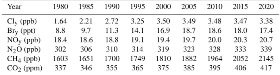
Table 1. Long-lived tracer amounts in the simulation (Austin and Butchart, 2003). Year 1980 1985 1990 1995 2000 2005 2010 2015 2020 Cly(ppb) 1.64 2.21 2.72 3.25 3.50 3.49 3.48 3.47 3.38 Bry(ppt) 8.8 9.7 11.3 14.1 16.9 18.7 18.6 18.0 17.4 NOy(ppb) 18.4 18.6 18.8 19.1 19.4 19.7 20.0 20.3 20.7 N₂O (ppb) 302 306 310 314 319 323 328 333 339 CH4(ppb) 1603 1651 1700 1749 1810 1882 1964 2052 2145 CO2(ppm) 337 346 355 365 375 385 395 406 417

observed in mid latitude NH ozone since the mid-1990s, which has been attributed both to changes in atmospheric dynamics (increased planetary wave driving) as well as de-creasing EESC. The reason for the change in dynamics is not fully understood, and could be either natural variability or driven by the climate change. The future evolution of the stratospheric ozone is therefore still uncertain.

The focus of this study is on climatological scale fea-tures such as regionally averaged seasonal ozone variations or year-to-year ozone variations in the high-latitude strato-sphere. We will present the results of a global 40-year mid-dle atmospheric simulation from 1980 until the end of 2019. We will show how the average high-latitude concentrations of stratospheric ozone, and ozone destruction have evolved during the past period (1980–1999), and how ozone is ex-pected to evolve in the near future (2000–2019). The strato-spheric processes affecting high latitude stratostrato-spheric ozone will also be analysed, and the trend analysis of the past and future periods will be shown and compared against measure-ments. The simulation has been performed with the global chemistry-transport model, FinROSE, described by Damski et al. (2007). For this study FinROSE model has been driven with the winds and temperatures from a transient simulation of the coupled chemistry climate model UMETRAC Austin and Butchart (2003), using specified concentrations of long-lived tracers such as the well-mixed greenhouse gases.

2 Simulation settings and driver data

FinROSE is a global 3-D grid point model (Damski et al., 2007), which is originally based on the NCAR-ROSE-model (Rose, 1983; Rose and Brasseur, 1989). FinROSE is an off-line chemistry transport model. The model includes 27 long-lived species/families and 14 species that are assumed to be in photochemical equilibrium. Chemistry includes around 110 gas-phase reactions, 37 photodissociation processes and 10 heterogeneous reactions. Photodissociation coefficients are compiled using the PHODIS radiative transfer model (Kylling, 1992; Kylling et al., 1997) and used through look-up tables. The aerosol and polar stratospheric cloud (PSC) processing includes liquid binary aerosols (LBA),

super-cooled ternary solutions (STS, PSC type Ib), nitric acid trihy-drates (NAT, PSC type Ia), NAT-rock and water ice particles (ICE, PSC Type II) and sedimentation. Chemical kinetics used in this work are updated to follow JPL-2002 (Sander et al., 2003). For the transport of the model constituents a flux-form Semi-Lagrange Transport-scheme (Lin and Rood, 1996) is used. For more detailed description of the FinROSE-model see (Damski et al., 2007).

The meteorology (i.e. winds and temperatures) used in this study was produced by the UMETRAC (Unified Model with Eulerian Transport And Chemistry). UMETRAC is a CCM based on the UK Met. Office’s Unified Model (Cullen, 1993). The ozone fields predicted by the chemistry in UME-TRAC are used in the model radiation scheme to couple the chemistry to the climate. In this study we have used a UMETRAC model integration completed for the period from January 1975 to January 2020 (Austin and Butchart, 2003). The integration was based on the use of observed sea surface temperatures and sea ice coverage for the past pe-riod (1980–2000). For the future pepe-riod (2000–2020) UME-TRAC used the results of a coupled ocean-atmosphere ver-sion of the Hadley Centres climate model (Williams, 2001).

The horizontal resolution in this 40-year FinROSE integra-tion was 5.00◦ _{by 11.25}◦ _{(latitude-longitude) with pole to}

pole latitudinal coverage. The vertical resolution of the sim-ulation was around 2700 m at 24 pressure levels from surface up to ∼0.15 hPa (or ∼62 km). The vertical grid of the model uses every other point of that used in UMETRAC. For the horizontal grid, the wind and temperature values are inter-polated from the UMETRAC three-dimensional daily values using bilinear interpolation. The vertical wind is solved in the FinROSE transport scheme.

The initial distributions of chemical constituents were taken directly from the UMETRAC integration. The boundary conditions were taken from UMETRAC monthly means. The chemical scheme in FinROSE does not include parametrizations for the source gases (e.g. CFCs and their chemistry). The concentrations of the long-lived tracers fol-lowed the projections defined in Austin and Butchart (2003). Halogen data and the well-mixed greenhouse gases are from Austin and Butchart (2003). The levels and expected future

evolutions of long-lived species, relevant to this study are shown in Table 1. Atmospheric concentrations of long-lived tracers (Table 1) are constrained at each timestep by relax-ation towards monthly mean zonal averages given by the driver model. The individual members in the chemical fami-lies (NOy, Clxand Bry), are constrained with respect to their

relative contributions given by the chemistry scheme. As a result of projections in well-mixed greenhouse gases and other long-lived constituents (Table 1) and chemistry cli-mate coupling in the driver model, the UMETRAC simu-lation captured the main characteristics of observed strato-spheric temperature trends and also indicated continued ing of the stratosphere in the near future. The Antarctic cool-ing trend in the past in the UMETRAC results also clearly in-dicated a strong connection between Antarctic ozone deple-tion and cooling of the stratosphere (see Austin and Butchart, 2003).

3 Transport characteristics of the 40-year CTM-simulation

The ability of a model to reproduce the stratospheric Brewer-Dobson circulation can be estimated using an analysis of the simulated age of air. This has become a standard way for testing stratospheric transport models in general (see Waugh and Hall (2002) for a review). In this study the age of air (hereafter also AOA) is defined as the average amount of time spent by the air parcels for the transportation from the source areas to any specific latitude and altitude in the stratosphere. The AOA diagnostic was used to see how the transport forc-ing, provided by the UMETRAC, works with the FinROSE transport scheme in comparison with the observed Brewer-Dobson circulation. As stated by Hall et al. (1999), in most CTMs the propagation of the annual atmospheric oscillations is too rapid in the vertical direction, and the CTMs also typi-cally underestimate the mean age of air throughout the strato-sphere.

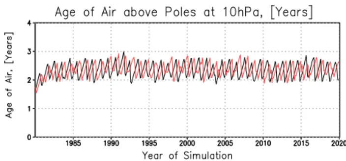
Figure 1 shows the evolution of the AOA tracer at the 10 hPa level in FinROSE over the North and South Pole. In-terannual variability is clearly seen in the peaks during the wintertime periods, as expected, with less interannual vari-ability during the summer. Over the South Pole the maxi-mum values are about three years, and the minimaxi-mum sum-mer values just below two years. Over the North Pole the maximum values are less than three years, and the minimum typically around two years. While the simulated general be-haviour follows what is expected from observations and the-ory, the absolute values are significantly lower than those given in Waugh and Hall (2002). The evolution of the AOA tracer is stable throughout the 40-year simulation period, but the model seems to have a Brewer-Dobson circulation which is unrealistically fast.

Fig. 1. The evolution of the age of air tracer above the South Pole

(black line) and North Pole (red line) at 10 hPa during the 40-year FinROSE simulation (in years).

4 Simulated global annual ozone distribution

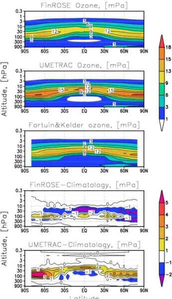
A comparison of the model results with the ozone climatol-ogy compiled by Fortuin and Kelder (1998) is shown in Fig. 2. This climatology is based on ozonesonde measure-ments and satellite measuremeasure-ments of ozone, covering the pe-riod from 1980 to 1991. In Fig. 2 the same pepe-riod was used for averaging the model results. The comparison shows that both models give reasonable and comparable results. How-ever, there are discrepancies between the simulations and ob-servations. The modelled ozone partial pressures are gener-ally lower than observed in FinROSE, and higher than ob-served in UMETRAC.

In general the ozone maxima in FinROSE ozone distribu-tion seems to be located higher up than in the measurements, while in the UMETRAC climatology the altitude matching seems to be better. The tropical ozone maximum in Fin-ROSE is clearly too weak while in UMETRAC the opposite is true. Over the high southern latitudes the FinROSE data is in line with the measurements, since both the altitude and the magnitude compares well. The ozone distribution in Fin-ROSE over the high northern latitudes is worse, as the partial pressure of ozone is too low while the height of the ozone maximum is reasonable. The height distribution of ozone in FinROSE yields to a lower column abundance, while in UMETRAC the higher partial pressure at more correct alti-tudes give too high ozone column abundances.

A general conclusion from Fig. 2 is that the FinROSE model reproduces the observed global patterns. The differ-ences between the two models, as well as between mod-els and measurements, seem to be connected with limita-tions and imperfeclimita-tions in the reproduction of the Brewer-Dobson circulation and with the differences in the strato-spheric chemistry formulations in these two models.

UMETRAC includes the coupling between transport char-acteristics and atmospheric composition through radiation, i.e. the changes in the composition due to the chemical processing are reflected in the simulated temperatures and winds. Since the simulated composition is in balance with

Fig. 2. Calculated model ozone climatologies for the period from

1980 to 1991, the measurement-based ozone climatology Fortuin and Kelder (1998), and respective differences. Values are shown as partial pressures (mPa).

the dynamics, one may say that UMETRAC produces its own balanced aeronomy. When the winds and temperatures from such a model are introduced to a CTM where the transport is formulated in similar way, but chemical formulations are different, the realized compositional patterns end up being qualitatively the same, but quantitatively different. As Fig. 2 shows, the ozone climatologies derived from FinROSE and UMETRAC have differences e.g. in magnitude and altitude of the tropical ozone maximum. The tropical maximum can be considered the starting point for the Brewer-Dobson cir-culation, as new stratospheric air is injected from the tro-posphere mainly over the tropics. In FinROSE the maxi-mum is located too high up, and in UMETRAC the tropical

ozone maximum is too strong, i.e. the reproduced Brewer-Dobson circulation in FinROSE has less ozone to start with, and transport towards the winter pole, while UMETRAC has too much. An offset in the ozone maximum during late win-ter to early spring, also affects ozone amounts during summer and autumn.

5 High latitude ozone evolution

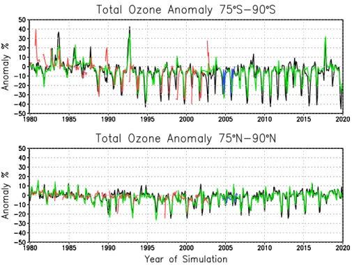
Figure 3 (upper panel) shows the percentage anomalies (from the 1980–1989 mean) in simulated total ozone enclosed by the 75th southern latitude for the 40-year simulation period in comparison to satellite-based TOMS-v8 and OMI total ozone measurements. Results from both the FinROSE and the UMETRAC simulations are shown. The FinROSE model reproduces all the observed main features, and the anomalies seen in the simulated ozone are of the same magnitude as in the TOMS measurements. The anomalies in the UMETRAC ozone are quite similar to the ones in FinROSE, although the total ozone levels are generally higher than measured.

In all cases the ozone hole starts to develop during July– August, and ozone recovery is complete by the end of November or early December, meaning that the ozone deple-tion caught by the FinROSE model is well timed. Another well-reproduced element in Fig. 3 upper panel is the grad-ual increase of the Antarctic ozone anomaly in both models. Antarctic springs that exhibit no or very weak ozone deple-tion occur the same years in FinROSE and UMETRAC. The UMETRAC and FinROSE transport schemes end up in very similar results, and therefore the driver model determines mainly year to year and season to season variability. The dif-ferences in absolute levels between the models derive mainly from the differences in chemical formulations.

During the future period of the simulation (in Fig. 3) both models exhibit similar patterns in the month-to-month ozone anomalies, as they do during the past period. A comparison between the anomalies seen during the past years (i.e. 1980 to 1999) and during the near future (i.e. from 2000 to 2019) suggests that in the near future the behaviour of ozone will be similar to that observed during the 1990s.

The ozone anomalies in the north are rather different from what is seen in the south as Fig. 3 shows. The overall multi-year monthly mean evolution in both models follows the ob-served seasonal patterns well. While not shown in Fig. 3, the modelled total ozone in FinROSE is about 40 DUs lower than the TOMS measurements during summer. Furthermore, in some cases during the winter-spring maximum, FinROSE gives over 100 DUs lower total ozone values than TOMS. In UMETRAC the summertime minima are regularly around 100 DUs higher, and the wintertime maximum are around 50 DUs higher than measured. Although the simulated age of air is too short, we may now conclude that the seasonal be-haviour in the general transport characteristics is reasonable

Fig. 3. Comparison of observed total ozone anomalies (from 1980–1989) with the modelled ozone anomalies. Time series are shown as

average values within the 75◦_{S latitude circle (upper panel) and 75}◦_{N latitude circle (lower panel). The anomalies in total ozone calculated}

from FinROSE data are presented by black lines, the UMETRAC anomalies as green lines, and the anomalies derived from the TOMS data by red lines and from OMI by blue lines.

and that there are clear similarities in the modelled interan-nual and seasonal patterns.

6 Ozone depletion

The processes causing ozone depletion require first of all formation of polar stratospheric clouds (i.e. PSCs), enough inorganic chlorine (and possibly other halogens) to be con-verted to active form, low enough stratospheric temperatures to cause denitrification, and finally, solar radiation to drive the actual ozone loss processes. The distribution of ozone is dependent on both atmospheric transport and chemistry. In order to have an approximate separation of these two main processes, we have formulated a passive ozone tracer, for which only the transport scheme of the model has been ap-plied. The passive ozone tracer is initialized twice every year, on 1st of June, and on 1st of December using the regular model ozone.

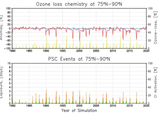
Time series of anomalies (from the 1980–1989 mean) in total nitrogen (NOy) and water vapour (H2O), the evolution

of chlorine activation (i.e. ClOx/Clx), and the difference

be-tween the passive ozone tracer (Tracer-O3) and model ozone

are shown in Fig. 4 for the whole 40-year time series together with the PSC exposure times (for types I and II). All values are based on monthly mean values within 75–90◦_{S, averaged}

over the vertical column from 146 to 31 hPa (i.e. between

ap-proximately 14 and 24 km). The time series show how some major processes are simulated in the model. Significant chlo-rine activation occurs during every austral winter-spring sea-son of this 40 year time series. The model simulates well the major chlorine activation, which occurs soon after the start of austral polar night. Chlorine activation starts as soon as the type-I PSCs appear. At the same time the level of total nitrogen, expressed by NOy, starts to decrease. The actual

ozone loss, as seen in Fig. 4 starts as the analysed area be-comes sunlit. This is seen as a deviation between the passive ozone tracer and model ozone. As the temperatures gradu-ally increase during the spring and the vortex disappears, the PSCs evaporate and the large-scale ozone depletion is typi-cally over by the end of November.

In the early 1980s the magnitude of the simulated ozone loss was at most between 50 and 60%. After the mid-1980s ozone depletion started to increase, frequently indicat-ing losses of more than 80% between 31 and 146 hPa. The fractional chlorine activation (in Fig. 4) was typically slightly larger during the 1980s than during 1990s and later decades. However, the total chlorine loading is lower in the 1980s and the net effect on ozone was low.

The rate of decrease of NOy, i.e. the rate of denitrification,

increases when the temperatures drop below the threshold for formation of ice particles. The relatively large PSC-type-II particles are formed and sedimented, which is seen as a

Fig. 4. Simulated evolutions for 1980-2019 of main constituents affecting ozone within 75◦_{S, and between 146 and 31 hPa. In the upper}

frame the percentage anomalies in total nitrogen is shown by the red line and in water vapour by the blue line. The relative difference between the passive ozone tracer and regular model ozone by yellow bars. In the lower frame the chlorine activation is shown by orange bars, the PSC type-I tracer is given by the green line and the PSC type-II tracer by the black line.

decrease in water vapour and especially in NOy. The

aver-age total nitrogen (NOy) between 146 and 31 hPa shows a

significant drop in connection to the occurrence of PSCs of type-II. Since conditions cold enough for the formation of ice particles exist during most of the winter-spring seasons, Fig. 4, the monthly average results do not exhibit any clear signs of significant denitrification caused by rapid sedimen-tation of large NAT particles (i.e. NAT rocks). However, this does not rule out the possible sedimentation of NAT rocks on a more local and shorter time scale.

Severe denitrification does not take place during every sin-gle simulated season. Exceptions are especially the years 1983 and 1992 when the decrease in total nitrogen shown by a positive anomaly, and also the ozone loss is smaller. Dur-ing these non ozone depletion cases the formation of ice is relatively moderate due to warmer conditions, which can be seen in the PSC exposure in Fig. 4. These warmer conditions may be connected to sudden stratospheric warming events which are known to be very rare in the Southern Hemisphere (see e.g. Shepherd et al., 2005). More likely, they illustrate problems in simulating model dynamics at the edges of the normal distribution.

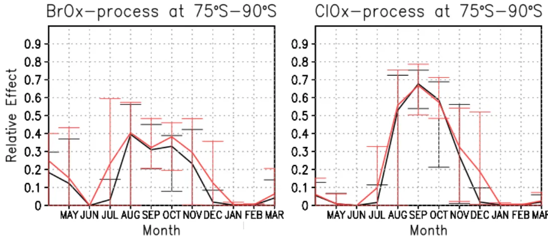
Figure 5 shows how the two main chemical ozone loss cy-cles have contributed to the simulated net ozone loss over Antarctica. The relative effect of catalytic ozone loss cycles by active chlorine (i.e. ClOx) is clearly the most significant.

During September these cycles are responsible for about 50 to 80% of the total ozone loss. The rest of the ozone depletion is due to the second most important catalytic cycle during the ozone hole season, namely the BrO-ClO cycle. The coupled ClO-BrO destruction of ozone is almost as important as the ClOxcycles during August and October. However, it should

be kept in mind that the amount of absolute ozone deple-tion itself is smaller during August as there is only a limited amount of solar radiation available within the analysed area. It is also worth noting that during other times of year, the catalytic cycles of NOx(summer), and HOx(autumn) are the

main contributors to ozone depletion (not shown). However, as seen from Fig. 5 these cycles do not contribute signifi-cantly to the chemical depletion of ozone during winter and spring.

Another way to analyse the 40-year time-series is to look at the total inorganic chlorine level in the atmosphere (see Table 1). Keeping in mind that since early 1980s the in-organic chlorine loading increased from about 1.6 to about 3.5 ppbvin the late 1990s, and that it is projected to remain

above 3 ppbvuntil the end of the 40-year simulation period,

a conclusion can be made: Chlorine activation, although a regular phenomenon, does not in itself lead to severe ozone depletion. After the winter season the high southern latitude stratosphere becomes sunlit and the active chlorine is rapidly deactivated if NO2 is present. This means that the amount

Fig. 5. A climatology showing the relative portions of the ozone loss chemistry due to the two main catalytic ozone loss cycles in FinROSE.

The left panel shows the effect of the ClOxprocessing and the right panel shows the effect of combined BrOx-ClOxchemistry. The past

period (1980–1999) is indicated with black lines and the future period (2000–2019) with red lines. The errorbars show the minimum and maximum portions during each month. The values are averaged within the 75◦_{S latitude, and between 146 and 31 hPa.}

of inorganic chlorine controls the potential severity of ozone depletion, and the occurrence and magnitude of PSCs and denitrification affects how long ozone depletion is prolonged in the spring.

The time series in Figs. 3 and 4 show that the increase in inorganic chlorine has made the ozone depletions more se-vere since the beginning of 1980s. The level of ozone de-pletion reached during the latter part of the 1990s seems to continue also during the future period. The two main factors are in place (i.e. the chlorine activation, and denitrification) throughout the whole 40-year simulation, while during the early years the actual levels of inorganic chlorine were lower, and therefore the ozone depletion was less severe. However, it is important to note that even with inorganic chlorine lev-els below 2 ppbv, large-scale ozone destruction may occur,

provided that the temperatures are low enough for extended periods of time leading to e.g. denitrification.

The situation in the winter and springtime northern high-latitude stratosphere is far less favourable for PSC forma-tion than in the south, as sufficiently low temperatures do not occur regularly. Time series of anomalies (from the 1980– 1989 mean) in total nitrogen (NOy) and water vapour (H2O),

the evolution of chlorine activation (i.e. ClOx/Clx), and the

difference between the passive ozone tracer (Tracer-O3) and

model ozone are shown in Fig. 6 for the whole 40-year time series together with the PSC exposure times (for types I and II). All values are based on monthly mean values within 75– 90◦_{N, averaged over the vertical column from 146 to 31 hPa}

(i.e. between approximately 14 and 24 km). As can be seen, these results differ from the Antarctic ones. While NOy

seems to exhibit some drops during the course of the simula-tion, the water vapour distribution is stable.

Interestingly, it seems that even on this average perspective chlorine activation of around 20 to 30% takes place during al-most every winter/spring. The level of chlorine activation is

clearly connected with the average existence of type-I PSCs, while in this averaged analysis no signs of type-II PSCs are found. The ozone loss exhibits no clear trend, except per-haps the increase during the first half of the 1980s. The cases of higher chlorine activations clearly coincide with the weak, but obvious, denitrifications and in turn with the ozone losses. It is quite clear that the low stratospheric tempera-tures provide the conditions for ozone depletion. Therefore, if the stratospheric temperatures would decrease as a result of the enhanced greenhouse effect, the probability for sig-nificant ozone loss may increase in the northern hemispheric high-latitudes.

In general, between 75◦_{N and 90}◦_{N, the total nitrogen}

does not exhibit as large a decrease as it does over Antarc-tica. This result is expected, as the temperatures are not low enough for ice-cloud formation. Since PSC type-II clouds are uncommon in the northern polar stratosphere, no exten-sive ozone depletion occurs. However, during some years stronger denitrification occurs, as the negative anomalies (from the 1980–1989 mean) in NOy reach values of about

50 to 60%. A closer look at the PSC-tracers also indicates that while there are no ice-form PSCs, type-I PSCs are seen during most of the winters since the mid 1980s.

Another interesting feature in these figures emerges if the behaviour of total nitrogen, water vapour, and the existence of ice-clouds are compared with each other. It seems that while there are no type-II PSCs, the NAT PSCs coincide with the stronger denitrifications. A logical conclusion is that the NAT particles have grown to sizes where significant sedi-mentation is possible. Denitrification occurs, but these low temperatures are not persistent enough for large scale deni-trifications. Nevertheless, during the most prominent years (e.g. 2000 or 2013) the drop in total nitrogen over the Arctic is calculated to be about 40%.

Fig. 6. Simulated evolutions for 1980-2019 of main constituents affecting ozone within 75◦_{N, and between 146 and 31 hPa. In the upper}

frame the percentage anomalies in total nitrogen is shown by the red line and in water vapour by the blue line. The relative difference between the passive ozone tracer and regular model ozone by yellow bars. In the lower frame the chlorine activation is shown by orange bars, the PSC type-I tracer is given by the green line and the PSC type-II tracer by the black line.

Figure 7 shows a climatology of how the different ozone loss processes have contributed to the net ozone loss in the north. During the northern hemispheric winter and spring the catalytic ozone loss cycles by active chlorine and bromine are almost equally significant as they are responsible for about 30 to 40% each of the total ozone loss. During the first half of the 1980s, processes other than chlorine destruction, or coupled bromine-chlorine destruction were dominant, i.e. the NOx-chemistry had a more significant role until the early

1990s (not shown). However, the absolute levels of ozone depletion were lower than after the mid 1980s. Furthermore, the previously shown timeseries (Fig. 6) suggests that during years with more significant ozone depletion, destruction by ClOxis the most important process.

In the Arctic stratosphere denitrification is clearly weaker than in the Antarctic, and therefore the net ozone depletion is also weaker in the 40-year simulation. However, as already stated for the Antarctic stratosphere, even a chlorine load-ing below 2 ppbvmay lead to significant large scale ozone

depletion if conditions for chlorine activation and denitrifi-cation prevail for long enough time periods. Therefore, the possible cooling of the Arctic stratosphere may give rise to more severe ozone depletion.

7 Ozone changes and trends

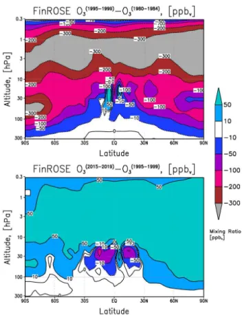
Figure 8 can be taken as a starting point for the analysis of the high latitude ozone changes. Ozone changes in the simulated data are shown as the difference between the climatology of 1980–1984 and the respective climatology of 1995–1999 (i.e. near past change). The near future change is shown as a dif-ference between the ozone climatology of 1995–1999 and the climatology of 2015–2019. Figure 8 shows these differ-ences in the mixing ratio. The past period difference shows a decrease in the ozone mixing ratios throughout the whole stratosphere. This difference has its maximum in the Antarc-tic polar stratosphere, being over 300 ppbv around 50 hPa.

While in the north the respective stratospheric decrease is about 100 to 150 ppbv, depending on the altitude. During the

future period, the model gives a slight increase of 50 ppbv

near 50 hPa, over the southern polar areas, and a similar in-crease in the upper stratosphere. Over the northern polar ar-eas an incrar-ease of the order of 50 ppbvis seen throughout the

whole stratosphere above 100 hPa. The results shown here will be discussed further below where the statistical signifi-cance of these changes will be assessed using trend analysis. Figure 9 shows the latitudinal distribution of average an-nual trend estimates from the FinROSE, TOMS (version 8) and UMETRAC total ozone for the past period (1980 to 1999). The trend estimates of both models for the near future

Fig. 7. A climatology showing the relative portions of the ozone loss chemistry due to the two main catalytic ozone loss cycles in FinROSE.

The left panel shows the effect of the ClOxprocessing and the right panel shows the effect of combined BrOx-ClOxchemistry. The past

period (1980–1999) is indicated with black lines and the future period (2000–2019) with red lines. The errorbars show the minimum and maximum portions during each month. The values are averaged within the 75◦_{N latitude, and between 146 and 31 hPa.}

period (2000–2019) are also shown. The trend estimates are calculated applying a standard linear regression to the monthly mean values. The trend errors, based on the Stu-dent’s T-test, are given for the 95% significance level. The overall agreement with measurements is good and both mod-els give similar trend estimates as obtained from the TOMS measurements.

For the past period, both actual values and uncertainty in-tervals of the FinROSE trends behave similarly as the TOMS trends. In the vicinity of 60◦_{S the decreasing annual average}

trend from FinROSE is only slightly less than the TOMS-derived trend. In the case of UMETRAC, the magnitude of the southern trends is somewhat smaller than the correspond-ing FinROSE trends, and the trend errors exhibit somewhat narrower error ranges.

Both models give large, statistically significant negative trends over the high polar latitudes. Over Antarctica the trend in the FinROSE data is almost −8%/decade and in the UMETRAC data the trend is about −6%/decade. Over the northern polar areas, FinROSE gives a trend of about −3.5%/decade, and UMETRAC about −5.5%/decade. The trends in polar ozone are well in line with the trend estimates shown by WMO (2003, Chapter 4, Figs. 4–31) Hadjinicolaou et al. (2002) or Fioletov et al. (2002).

The average annual trend estimates for the future period (in Fig. 9) are similar for both models over the high south-ern latitudes. Both models exhibit small but statistically in-significant positive trends of 2 to 3% per decade. Over the northern polar areas the results of the two models are almost the same. The UMETRAC trend estimates give a positive trend of about 3%/decade, which is significant at the 95% confidence level. FinROSE gives nearly the same trend with a somewhat larger error range and the trend is also signifi-cant at the 95% level. From an annual average perspective

Fig. 8. Ozone changes in average annual zonal distributions. Top

panel gives the change between 1980–1985 and 1995–1999. Lower panel shows the difference between 1995–1999 and 2015–2019. Values are shown as mixing ratios.

Fig. 9. Annually averaged total ozone trends [%/decade]. The errorbars indicate the 95% confidence intervals, calculated using the Student’s

T-test.

the results from both models suggest that a small increase in total ozone may take place over high southern latitudes by 2019. However, the statistical significance is low imply-ing that the ozone depletion may remain on a similar level to what was seen in the 1990s. Over the northern polar areas, on an annual average basis, a statistically significant positive trend is simulated, which could be a sign of a start of ozone recovery. These results are in line with those presented in Fig. 8.

Figure 10 shows the latitudinal distributions of seasonal total ozone trend estimates of FinROSE and TOMS for the past period and FinROSE for the future period. As for the annual average trend estimates, the seasonal trend estimates from FinROSE are also in good or reasonable agreement with the TOMS trends. During the northern winter months (i.e. December, January, and February) over northern high lati-tudes the modelled trends are between −5 and −8%/decade, being significantly different from zero at the 95% confidence level. During the spring months (March through May) at high northern latitudes, the model agrees reasonably well with the measured trends. While TOMS gives a significant negative trend of around −7%/decade, FinROSE reproduces a trend of around −5%/decade, which agrees with the observations at the 95% confidence level.

The southern high latitude trends, shown in Fig. 10 left and middle panels follow the observation based trends. During

the austral winter (June–August), the model reproduces the observed trends well. During the austral spring (September– November), the most visible feature is the large, statistically significant (at the 95% confidence level) negative trend of to-tal ozone. At about 80◦_{S, the TOMS and FinROSE trend}

estimates agree with a trend of about −18%/decade. Fin-ROSEs trend errors are in good agreement with the TOMS trend errors, suggesting that the interannual variability sim-ulated by FinROSE is also of the same order. It is interest-ing to note that a typical problem of model simulations over the northern mid-latitudes is also evident here. The northern hemisphere mid-latitude negative ozone trend, which peaks between 45–50◦_{N and then reduces toward 60}◦_{N (e.g.}

Had-jinicolaou et al., 2005) is not well simulated.

In Fig. 10 (right panel) the seasonal trend estimates for lat-itudinal total ozone behaviour in the near future (2000–2019) are shown. It can be seen that the winter and spring total ozone will increase over the poles. For the Arctic winter-spring seasons this increase is around 3 to 5%/decade, and in the south for the austral winter-spring, the increase is about 2 to 3%/decade. The FinROSE results indicate that the negative ozone trends are levelling off during the near future. Since the positive trends in winter and spring high latitudes, calculated from the FinROSE results, are not sig-nificant, we can conclude (supported by e.g. Weatherhead et al., 2000; Austin and Butchart, 2003; Weatherhead and

Fig. 10. Seasonally averaged total ozone trends [%/decade] of TOMS observations for the period 1980-1999 and of FinROSE for period

1980–1999 and 2000–2019. The error bars indicate the 95% confidence intervals, calculated using the Student’s T-test.

Andersen, 2006) that no unambiguous recovery of the ozone is likely to be seen before 2020. The results of Austin and Butchart (2003), as well as those in Austin et al. (2003b) also suggested that the turnover of ozone trends would start in about 2005. The results presented here support those con-clusions.

Figure 11 shows vertical cross-sections of the simulated seasonal trends in FinROSE for the past period, focusing on high latitudes. In the past negative trends between 250 and 10 hPa are typical during all seasons. During the northern hemispheric winter, the statistically most signifi-cant (95% confidence, or more) trends are between −5 and

Fig. 11. Vertical distributions of the seasonal ozone concentration trends [%/decade] for the past period (1980–1999). The significance levels

are indicated with dotted black lines for 90% significance, with dashed for 95% significance, and with solid black line for 99% significance.

−10%/decade above 100 hPa, and north of the 65◦N lati-tude. The maximum trend in the northern hemispheric winter is, however, located between 250 and 150 hPa, being about −15%/decade (without statistical significance). This large negative trend is associated with trends in tropopause height, and is further discussed below. In the northern hemispheric spring the decreasing trend in the lower stratosphere above 40 hPa disappears while the negative trend below 40 hPa stays negative. Similarly to the winter trend estimates, a sta-tistically significant trend between −5 and −10%/decade is found between 150 and 50 hPa, while the maximum neg-ative trend of about −15%/decade is located between 250 and 150 hPa. In the spring, this upper tropospheric to lower stratospheric trend is significant at the 90% level north of 75◦_N.

Over the southern hemispheric high latitudes (in Fig. 11) the winter trend estimates are somewhat different. While negative trends are typical over the whole domain, the statis-tical significance of the negative ozone trends south of 75◦_S,

and below 10 hPa, is weak. At the 95% significance level a trend between −5 and −10%/decade is found only between 25 and 10 hPa, and the statistically most significant trends are seen south of 75◦_{S around 25 hPa. During the}

Antarc-tic spring, ozone is depleted with estimated trends more than −40%/decade south of the 75◦S latitude between 150 and 50 hPa. The estimated trends are also significantly different from zero at the 99% level, and are related to the increasing halogen amounts (Table 1). These seasonal trend estimates are also in agreement with the observed trend estimates pre-sented by Randel and Wu (1999).

Fig. 12. Vertical distributions of the seasonal ozone concentration trends [%/decade] for the future period (2000–2019). The significance

levels are indicated with dotted black lines for 90% significance, with dashed for 95% significance, and with solid black line for 99% significance.

Simulated trends for the future period are shown in Fig. 12. A very general conclusion of the northern polar stratospheric ozone trends is that they are slightly positive, but statistically not significant within the polar area. The same is true in the case of southern hemispheric wintertime trends (i.e. June to August). During the austral spring a small negative trend of ozone is found close to 30 hPa south of 70◦_{S, although}

with-out statistical significance. According to WMO (2003) the decrease in the atmospheric chlorine loading will lead to a gradual recovery of the stratospheric ozone over the next 50 years. No clear signal of the start of the recovery of ozone is seen during the first two decades of the 21st century. How-ever, the results from FinROSE do show that the ozone levels

off during the last two decades of the simulation. The strato-spheric cooling due to the climate change has a potential for enhancing the polar ozone depletion. However, based on the analyses of the ozone trends alone, it is not straightforward to say, whether this mechanism is seen in these results or not. The negative ozone trend close to the tropopause in high northern latitudes during winter and spring, shown in Fig. 11 is in line with a number of recent studies (see e.g. WMO, 2003). The observed dependence of the column ozone on the tropopause height is well documented, although the level of understanding is still somewhat limited. In gen-eral, the observations have shown that the northern hemi-spheric tropopause at mid- and high-latitudes have risen

during the past few decades, which imply decreases in to-tal ozone. Austin et al. (2003a) have shown that in the driver model (i.e. UMETRAC), a statistically significant decrease in tropopause pressures is exhibited over a wide range of latitudes. Furthermore, over the mid-latitudes this negative trend is about 1 hPa/decade, which in turn is in line with ob-servations and other model changes (Santer et al., 2003). In WMO (2003) it was concluded that these trends are not due to the changes in stratospheric ozone, and thus radiatively driven, but due to the changes in tropospheric circulation. As a conclusion, it may be stated that the FinROSE sim-ulation also exhibits this observed connection between the tropopause height and ozone.

8 Discussion

The quality of CTM studies is very much dependent on the transport characteristics, the quality of the driver fields, as well as on the chemistry scheme of the CTM. With respect to this study, the uncertainties associated with the CCM have been discussed by Austin et al. (2003b). The shortcomings in the realized Brewer-Dobson circulation, and the large natural variability of the northern polar vortex, increased the uncer-tainty of the trend analyses in this study. The problems in the age of air distribution and the Brewer-Dobson circulation, are well-known features of CTMs (Hall et al., 1999).

Every model produces its own aeronomy, and its own balances between radiation driven processes, dynamically driven processes, and chemistry driven processes. This means that in the case of dynamically-driven atmospheric processes, the patterns reproduced by FinROSE follow those in the driver simulation, which in turn are dependent on the radiation couplings or used WMGHG projections in the CCM itself. In the case of chemistry-driven processes, like the springtime Antarctic ozone hole, the FinROSE model is capable of making a more independent representation. In general, the results presented here indicate that the ozone evolution is more predictable in the winter-spring Antarctic stratosphere than in the Arctic stratosphere where the natural interannual variability is greater.

Since the analyses in this study are based on average quan-tities (i.e. zonal averages, monthly means etc.), we have not discussed all the fine-scale features that the simulation con-tains. The inclusion of the effects caused by large NAT par-ticles (i.e. sedimentation and denitrification) clearly have an effect on the results exhibited in this study, as the moderate Arctic denitrifications are being reproduced in the absence of ice particles. These results suggest, in line with other studies (e.g. WMO, 2003), that the denitrification caused by gravita-tional settling of ice particles is not causing denitrifications over the Arctic. While there was evidence of denitrifications due to large NAT PSC sedimentation, the threshold for the ice-formation was not crossed.

From the Antarctic perspective, as the temperatures below the frostpoint are observed on annual basis during winter, the process of PSC sedimentation is relatively straightforward. However, as shown by Fahey et al. (2001), and further stud-ied by Carslaw (2002), under persistent conditions the NAT-type PSCs may also grow as large as 10 to 20 µm, and there-fore cause significant denitrifications due to sedimentation. This phenomena can be of great importance in the winter-time northern polar stratosphere where temperatures below ice frostpoint are uncommon. According to WMO (2003), the largest uncertainties in stratospheric model studies of ozone depletion are due to the unrealistic representation of denitrification processes. In order to have a more realistic description, especially in the Arctic, the 40-year simulation presented in this study takes into account denitrification ef-fects resulting from the growing of the NAT particles to sizes where sedimentation may become truly effective. However, since this work is based on a single simulation, and focuses on the analysis of climate-scale average quantities, it is not straightforward to make conclusions on the effect of the more detailed treatment of denitrification.

In the Arctic stratosphere, chlorine activation is an annual phenomenon. However, since the conditions in the Arctic polar vortex are less severe than in the Antarctic, no large scale Antarctic-like ozone depletion is seen in the simula-tion before the end of 2019. It is also possible that more local ozone perturbations may cause elevated levels of UV over the populated northern hemisphere high-latitude areas if the ozone depletion affects the ozone distributions dur-ing the followdur-ing summer as well. This matter has recently been addressed by Fioletov et al. (2005). Recently, quan-titative relations between the stratospheric temperatures and the Arctic springtime ozone losses were found and discussed by Rex et al. (2004). Based on the observations, it was shown that in the stratosphere, for each Kelvin cooled, a 15 DU total column ozone reduction is realized. Further signif-icant depletion could occur if the temperatures in the Arc-tic reach ice-formation temperatures on larger scales before the chlorine loading has reduced below 2 ppbv. Here the

early 1980s ozone depletion events are important references. As was noted before, even chlorine levels below 2.1 ppbv

may cause large-scale ozone depletion. Whether the regula-tions in the Montreal protocol (UNEP , 2000) are enough in a colder stratosphere remains unanswered in this work. The level of chlorine remains above 3 ppbvduring the timeframe

of this study (i.e. 1980–2019), therefore a longer simulation timeframe would be needed. The Antarctic ozone depletions are expected to continue as severe as they are at present until the end of 2019.

9 Summary and conclusions

Off-line Chemical Transport Models (CTMs) driven by externally provided wind and temperature fields are very

useful for the studies of atmospheric processes on various timescales. The main purpose of this study was to use the winds and temperatures resulting from a 40-year coupled chemistry climate model simulation, to drive the FinROSE chemistry transport model for the study of the past and fu-ture behaviour of the ozone layer. Global CTMs have mostly been used for multi-year simulations of the stratosphere us-ing observational based meteorologies (e.g. analyses of nu-merical weather prediction models, like the ECMWF model). The results presented and discussed in this paper should be considered, first of all, as a proof for the applicability of the combined CTM-CCM approach itself in climate scale stud-ies, as well as a documentation of the 40-year simulation. The advantages of using the off-line chemistry transport ap-proach with externally specified winds and temperatures, are abundantly cost-beneficial. More effort can be put to the rep-resentativeness of the chemistry solvers and output diagnos-tics. Therefore, the CTMs provide an affordable platform for the studies of individual atmospheric processes and add value to the chemistry coupled climate model integrations. Our general conclusion is therefore that this approach pro-vides an efficient tool with which to explore the long term chemistry of the stratosphere both during the past and for the future.

In order study the effect of stratospheric cooling on ozone depletion we showed how the average polar concentrations of stratospheric ozone, and processes leading to the high latitude ozone destruction evolved in our simulation during the past (1980–1999) and near future (2000–2019) periods. We also compared our results with measurements, and per-formed a trend analysis for the past and future periods. Sum-marizing the overall results of the 40-year CTM simulation we may state that the simulated patterns in the near past agreed well with the observed patterns and trend estimates opening the way for the conclusions about the future. The results of this study suggest that the extent of seasonal ozone depletion over both northern and southern high-latitudes are near a maximum and that while climate change might cool the lower stratosphere, the cooling in this simulation did not accelerate high latitude ozone depletion significantly. The recovery of seasonal high latitude ozone losses is not to take place for the next 15 years, emphasizing the need for longer model integrations for the predictions of ozone recovery.

Acknowledgements. The authors are grateful to the Ozone

Pro-cessing Team at the NASA Goddard Space Flight Center for the TOMS V8 column ozone, and to the OMI groups at FMI, KNMI and NASA for the OMI column ozone data. The authors wish to thank Prof. G. Brasseur for providing the original model code and valuable guidance. The funding received through the EU projects EuroSPICE (EVK2-CT-1999-00014) and CANDIDOZ (EVK2-CT-2001-00133) is gratefully acknowledged. We are also thankful for the funding received from the Academy of Finland through the projects FAUVOR II and FARPOCC.

Edited by: M. Dameris

References

Austin, J.: A Three-Dimensional Coupled Chemistry-Climate Model Simulation of Past Stratospheric Trends, J. Atmos. Sci., 59, 2, 218–232, 2002.

Austin, J. and Butchart N.: Coupled chemistry-climate model sim-ulations for the period 1980 to 2020: Ozone depletion and the start of ozone recovery, Q. J. Roy. Meteorol. Soc., 129, 3225– 3249, 2003.

Austin, J., Butchart, N., Claud, C.,, Cagnazzo, C., Hauchecorne, A., Hampson, J., Kaurola, J., Damski, J., Th¨olix, L., Langematz, U., Mieth, P., Nissen, K., Grenfell, L., Lahoz, W., Hare, S., and Canziani, P.: EuroSPICE: The European Project on Stratospheric Processes and their Influence on Climate and the Environment – Description and brief Highlights, in: SPARC Newsletter No. 21, July 2003, pp. 15–19, 2003.

Austin, J., Shindell, D., Bruhl, C., Dameris, M., Manzini, E., Na-gashima, T., Newman, P., Pawson, S., Pitari, G., Rozanov, E., Schnadt, C., and Shepherd, T. G.: Uncertainties and assessments of chemistry-climate models of the stratosphere, Atmos. Chem. Phys., 3, 1–27, 2003,

http://www.atmos-chem-phys.net/3/1/2003/.

Austin, J. and Wilson, R.J.: Ensemble simulations of the de-cline and recovery of stratospheric ozone J. Geophys. Res., 111, D16314, doi:10.1029/2005JD006907, 2006.

Brasseur, G. P., Tie, X., Rasch, P., and Lef`evre, F.: A three-dimensional model simulation of the Antarctic ozone hole: Im-pact of anthropogenic chlorine on the lower stratosphere and up-per troposphere, J. Geophys. Res., 102, 8909–8930, 1997. Carslaw, K. S., Kettleborough, J. A., Northway, M. J., Davies, S.,

Gao, R., Fahey, D. W., Baumgardner, D. G., Chipperfield, M. P., and Kleinb¨ohl, A.: A vortex-scale simulation of the growth and sedimentation of large nitric acid hydrate particles, J. Geophys. Res., 107(D20), 8300, doi:10.1029/2001JD000467, 2002. Chipperfield, M. P.: Multiannual simulations with a

threedimen-sional chemical transport model, J. Geophys. Res., 104, 1781– 1805, 1999.

Chipperfield, M. P.: A three-dimensional model study of long-term mid-high latitude lower stratosphere ozone changes, Atmos. Chem. Phys., 3, 1253–1265, 2003,

http://www.atmos-chem-phys.net/3/1253/2003/.

Cullen, M. J. P.: The unified forecast/climate model, Meteorol. Mag., 122, 81–94, 1993.

Damski, J., Th¨olix, L., Backman, L., Taalas, P., and Kulmala, M.: FinROSE – Middle Atmospheric Chemistry Transport Model, Boreal Environ. Res., in press, 2007.

Dhomse, S., Weber, M., Wohltmann, I., Rex, M., and Burrows, J. P.: On the possible causes of recent increases in northern hemi-spheric total ozone from a statistical analysis of satellite data from 1979 to 2003, Atmos. Chem. Phys., 6, 1165–1180, 2006, http://www.atmos-chem-phys.net/6/1165/2006/.

Egorova, T. A., Rozanov, E., Schlesinger, M., Andronova, N., Malyshev, S., Karol, I., and Zubov, V.: Assessment of the effect of the Montreal Protocol on atmospheric ozone, Geophys. Res. Lett., 28(12), 2389–2392, doi:10.1029/2000GL012523, 2001. Eyring, V., Butchart, N., Waugh, D. W., et al.: Assessment of

tem-perature, trace species and ozone in chemistry-climate model simulations of the recent past, J. Geophys. Res., 111, D22308, doi:10.1029/2006JD007327, 2006.

P. J., Northway, M. J., Holecek, J. C., Ciciora, S. C., McLaugh-lin, R. J., Thompson, T. L., Winkler, R. H., Baumgardner, D. G., Gandrud, B., Wennberg, P. O., Dhaniyala, S., McKinney, K., Pe-ter, Th., Salawitch, R. J., Bui, T. P., Elkins, J. W., WebsPe-ter, C. R., Atlas, E. L., Jost, H., Wilson, J. C., Herman, R. L., Kleinb¨ohl, A., and von K¨onig, M.: The detection of large nitric-acid parti-cles in the winter Arctic stratosphere, Science, 291, 1026–1031, 2001.

Fioletov, V. E., Bodeker, G. E., Miller, A. J., McPeters, R. D., and Stolarski, R.: Global and zonal total ozone variations estimated from ground-based and satellite measurements: 1964–2000, J. Geophys. Res., 107(D22), 4647, doi:10.1029/2001JD001350, 2002.

Fioletov, V. E. and T. G. Shepherd: Summertime total ozone vari-ations over middle and polar latitudes, Geophys. Res. Lett., 32, L04807, doi:10.1029/2004GL022080, 2005.

Fortuin, J. P. F. and Kelder, H.: An ozone climatology based on ozonesonde and satellite measurements, J. Geophys. Res., 103(D24), 31 709–31 734, doi:10.1029/1998JD200008, 1998. Garcia, R. R., Marsh, D., Kinnison, D., Boville, B., and Sassi, F.:

Simulation of secular trends in the middle atmosphere 1950– 2003, J. Geophys. Res., 111, doi:10.1029/2006JD007485, in press, 2007.

Hadjinicolaou, P., Jrrar, A., Pyle, J. A., and Bishop, L.: The dynam-ically driven long-term trend in stratospheric ozone over northern mid-latitudes, Q. J. Roy. Meteor. Soc., 128, 1393–1412, 2002. Hadjinicolaou P., Pyle, J. A., and Harris, N. R. P.: The recent

turnaround in stratospheric ozone over northern middle latitudes: A dynamical modeling perspective, Geophys. Res. Lett., 32, L12821, doi:10.1029/2005GL022476, 2005.

Hall, T. M., Waugh, D. W., Boering, K. A., and Plumb, R. A.: Eval-uation of transport in atmospheric models, J. Geophys. Res., 104, 18 815–18 839, 1999.

Kylling, A.: Radiation transport in cloudy and aerosol loaded atmo-sphere, Ph.D. thesis, University of Alaska, 1992.

Kylling, A., Albold, A., and Seckmeyer, G.: Transmittance of a cloud is wavelength – dependent in the UV-range: Physical interpretation, Geophys. Res. Lett., 24(4), 397–400, doi:10.1029/97GL00111, 1997.

Lin, S.-J. and Rood R. B.: Multidimensional flux-form semi-lagrangian transport schemes, Mon. Wea. Rev., 124, 2046–2070, 1996.

Manzini, E., Steil, B., Br¨uhl, C., Giorgetta, M. A., and Kr¨uger, K.: A new interactive chemistry-climate model: 2. Sensitivity of the middle atmosphere to ozone depletion and increase in green-house gases and implications for recent stratospheric cooling, J. Geophys. Res., 108(D14), 4429, doi:10.1029/2002JD002977, 2003.

Nagashima, T., Takahashi, M., Takigawa, M., and Akiyoshi, H.: Future development of the ozone layer calculated by a general circulation model with fully interactive chemistry, Geophys. Res. Lett., 29(8), doi:10.1029/2001GL014026, 2002.

Randel, W. J. and Wu, F.: A stratospheric ozone trends data set for global modeling studies, Geophys. Res. Lett., 26, 3089–3092, 1999.

Reinsel, G. C., Miller, A. J., Weatherhead, E. C., Flynn, L. E., Na-gatani, R. M., Tiao, G. C., and Wuebbles, D. J.: Trend analysis of total ozone data for turnaround and dynamical contributions, J. Geophys. Res., 110, D16306, doi:10.1029/2004JD004662, 2005.

Rex, M., Salawitch, R. J., von der Gathen, P., Harris, N. R. P., Chipperfield, M. P., and Naujokat, B.: Arctic ozone loss and climate change, Geophys. Res. Lett., 31, L04116, doi:10.1029/2003GL018844, 2004.

Rose, K.: On the influence of nonlinear wave-wave interaction in a 3-d primitive equation model for sudden stratospheric ings, Con-tributions to Atmospheric Physics, 56, 1, 14–41, 1983.

Rose K. and Brasseur, G.: A three-dimensional model of chemically active trace species in the middle atmosphere during disturbed winter conditions, J. Geophys. Res., 94(D13), 16 387–16 403, 1989.

Rummukainen, M., Isaksen, I. S. A., Rognerud, B., and Stordal,F., A global model tool for three-dimensional multiyear strato-spheric chemistry simulations: Model description and first re-sults, J. Geophys. Res., 104, 26 437–26 456, 1999.

Sander, S. P., Ravishankara, A. R., Friedl, R. R., et al.: Chemical Kinetics and Photochemical Data for Use in Atmospheric Stud-ies, Evaluation Number 14, JPL Publ. 02-25, 2003.

Santer, B. D., Sausen, R., Wigley, T. M. L., Boyle, J. S., AchutaRao, K., Doutriaux, C., Hansen, J. E., Meehl, G. A., Roeckner, E., Ruedy, R., Schmidt, G., and Taylor, K. E.: Behavior of tropopause height and atmospheric temperature in models, re-analyses, and observations: Decadal changes, J. Geophys. Res., 108, 4002, doi:10.1029/2002JD002258, 2003.

Shepherd, T. G., Plumb, R. A., and Wofsy, S. C.: Preface to JAS Special Issue on the Antarctic Stratospheric Sudden Warming and Split Ozone Hole of 2002, J. Atmos. Sci., 62, 565–566, 2005. Steil, B., Br¨uhl, C., Manzini, E., Crutzen, P. J., Lelieveld, J., Rasch, P. J., Roeckner,E., and Kr¨uger, K.: A new interactive chemistry-climate model: 1. Present-day climatology and inter-annual variability of the middle atmosphere using the model and 9 years of HALOE/UARS data, J. Geophys. Res., 108(D9), 4290, doi:10.1029/2002JD002971, 2003.

Steinbrecht, W., Claude, H., Sch¨onenborn, F., McDermid, I. S., Leblanc, T., Godin, S., Song, T., Swart, D. P. J., Meijer, Y. J., Bodeker, G. E., Connor, B. J., K¨ampfer, N., Hocke, K., Calisesi, Y., Schneider, N., de la No¨e, J., Parrish, A. D., Boyd, I. S., Br¨uhl, C., Steil, B., Giorgetta, M. A., Manzini, E., Thomason, L. W., Za-wodny, J. M., McCormick, M. P., Russell, J. M., III, Bhartia, P. K., Stolarski, R. S., and Hollandsworth-Frith, S. M.: Long-term evolution of upper stratospheric ozone at selected stations of the Network for the Detection of Stratospheric Change (NDSC), J. Geophys. Res., 111, D10308, doi:10.1029/2005JD006454, 2006. Tian, W. and Chipperfield, M. P.: A New coupled chemistry-climate model for the stratosphere: The importance of coupling for future O3-climate predictions, Q. J. Roy. Meteor. Soc., 131, 281–303, 2005.

UNEP: The Montreal Protocol on Substances that Deplete the Ozone Layer as adjusted and/or amended in in London 1990, Copenhagen 1992, Vienna 1995, Montreal 1997, Beijing 1999, Ozone Secretariat, United Nations Environment Programme, http://www.unep.org/ozone, 2000.

Waugh, D. and T. Hall: Age of stratospheric air: The-ory, observations, and models, Rev. Geophys., 40(4), 1010, doi:10.1029/2000RG000101, 2002.

Weatherhead, E. C. and S. B. Andersen: The search for signs of recovery of the ozone layer. Nature, 441, 39–45, doi:10.1038/nature04746, 2006.

Bishop, L., Hollandsworth Frith, S. M., DeLuisi, J., Keller, T., Oltmans, S. J., Fleming, E. L., Wuebbles, D. J., Kerr, J. B., Miller, A. J., Herman, J., McPeters, R., Nagatani, R. M., and Frederick, J. E.: Detecting the recovery of total column ozone, J. Geophys. Res., 105, 22 201–22 210, 2000.

Williams, K. D., Senior, C. A., and Mitchell, J. F. B., Transient climate change in the Hadley Centre models: the role of physical processes, J. Climate, 14, 2659–2674, 2001.

WMO, Scientific Assessment of Ozone Depletion: 2002, Global Ozone Research and Monitoring Project, Report No. 47, 498 pp., Geneva, 2001.

Wohltmann, I., Rex, M., Brunner, D., and M¨ader, J.: Integrated equivalent latitude as a proxy for dynamical changes in ozone column, Geophys. Res. Lett., 32, L09811, doi:10.1029/2005GL022497, 2005.

Yang E.-S., Cunnold, D. M., Salawitch, R. J., McCormick, M. P., Russell III, J., Zawodny, J. M., Oltmans, S., and Newchurch, M. J.: Attribution of recovery in lower-stratospheric ozone, J. Geophys. Res., 111, D17309, doi:10.1029/2005JD006371, 2006.