MRI assessment of multiple dipolar relaxation time ( T 1 D ) components in biological tissues interpreted with a generalized inhomogeneous magnetization transfer (ihMT) model

HAL Id: hal-02456394

https://hal-amu.archives-ouvertes.fr/hal-02456394

Submitted on 27 Jan 2020

HAL is a multi-disciplinary open access

archive for the deposit and dissemination of

sci-entific research documents, whether they are

pub-lished or not. The documents may come from

teaching and research institutions in France or

L’archive ouverte pluridisciplinaire HAL, est

destinée au dépôt et à la diffusion de documents

scientifiques de niveau recherche, publiés ou non,

émanant des établissements d’enseignement et de

recherche français ou étrangers, des laboratoires

MRI assessment of multiple dipolar relaxation time ( T

1 D ) components in biological tissues interpreted with a

generalized inhomogeneous magnetization transfer

(ihMT) model

Victor N.D. Carvalho, Andreea Hertanu, Axelle Grélard, Samira Mchinda,

Lucas Soustelle, Antoine Loquet, Erick Dufourc, Gopal Varma, David Alsop,

Pierre Thureau, et al.

To cite this version:

Victor N.D. Carvalho, Andreea Hertanu, Axelle Grélard, Samira Mchinda, Lucas Soustelle, et al..

MRI assessment of multiple dipolar relaxation time ( T 1 D ) components in biological tissues

inter-preted with a generalized inhomogeneous magnetization transfer (ihMT) model. Journal of Magnetic

Resonance, Elsevier, 2020, 311, pp.106668. �10.1016/j.jmr.2019.106668�. �hal-02456394�

MRI assessment of multiple dipolar relaxation time (T

1D

)

components in biological tissues interpreted with a generalized

inhomogeneous magnetization transfer (ihMT) model.

Victor N. D. Carvalho

_{, Andreea Hertanu}

_{, Axelle Gr´elard}

_{, Samira Mchinda}

_{, Lucas}

Soustelle

_{, Antoine Loquet}

_{, Erick J. Dufourc}

_{, Gopal Varma}

_{, David C. Alsop}

_{, Pierre}

Thureau

_{, Olivier M. Girard}

_{, and Guillaume Duhamel}

1_{Aix Marseille Univ, CNRS, CRMBM UMR 7339, Marseille, France} 2_{Aix Marseille University, CNRS, ICR UMR 7273, Marseille, France} 3_{CBMN UMR 5248, CNRS University of Bordeaux, Bordeaux INP, Pessac, France}

4_{Department of Radiology, Division of MR Research, Beth Israel Deaconess Medical Center, Harvard Medical} School, Boston, MA, United States

T1D, the relaxation time of dipolar order, is sensitive to slow motional processes. Thus T1D is a probe for membrane dynamics and organization that could be used to characterize myelin, the lipid-rich membrane of axonal fibers. A mono-component T1D model associated with a modified ihMT sequence was previously proposed for in vivo evaluation of T1D with MRI. However, experiments have suggested that myelinated tis-sues exhibit multiple T1Dcomponents probably due to a heterogeneous molecular mobility. A bi-component T1D model is proposed and implemented. ihMT images of ex-vivo, fixed rat spinal cord were acquired with multiple frequency alternation rate. Fits to data yielded two T1Ds of about 500 µs and 10 ms. The proposed model seems to further explore the complexity of myelin organization compared to the previously reported mono-component T1D model.

Keywords: Dipolar relaxation time; T1D; Inhomogeneous magnetization transfer; ihMT; MRI contrast; Jeener-Broekaert; Myelin; Myelin Imaging.

1

Introduction

Dipolar relaxation has recently regained attention in MRI with the discovery of a new imaging modality, inhomogeneous Magnetization Transfer (ihMT) [1], which allows isolating the contribution of dipolar order e↵ects to magnetization transfer occurring within broad macromolecular lines [2–4]. The ihMT technique is intrinsically weighted by T1D, the dipolar relaxation time, hence providing a new endogenous contrast to characterize biological tissues in vivo. Although dipolar order and associated relaxation have been studied quite extensively in chemical physics [5–8], especially in the field of liquid crystals and organic crystals, little is known about this yet unexplored relaxation mechanism in biological tissues.

Similar to T1 and T2 spin relaxation mechanisms, T1D relaxation is driven by molecular motions and can in principle deliver quantitative information about molecular dynamics and organization, which are related to motional correlation times and activation energy [9, 10]. Yet, as compared to T1, T1D is specifically sen-sitive to slower motional processes occurring within a frequency range corresponding to the magnitude of the local dipolar field !d, and on the order of 1-20 kHz depending on the motional averaging of the dipolar

⇤_{Corresponding author: G. Duhamel. Aix Marseille Univ, CNRS, CRMBM UMR 7339, 27 bd Jean Moulin, 13385 Marseille,}

interactions. Formally this may be expressed as an additional relaxation term involving the spectral density of molecular motions at the local field frequency J(!d) [7, 11, 12]. This term indicates that T1D will reach a minimum for correlation times on the order of 1/!d, corresponding to motions that are most efficient to catalyze (e.g. shorten) relaxation. Of interest, T1D has been shown to be sensitive to membrane collective motions [13, 14] rather than intramolecular motions, which occur at much higher rate. As collective motions in a membrane could be probed to evaluate membrane fluidity and elasticity, T1D measurement with MRI could potentially provide in vivo quantification of these biological features. This is an interesting application for studying myelin, a lipid-protein (70%/30% of dry matter) multi-lamellar membrane [15], since assessing myelin fluidity may yield further understanding of demyelinating diseases, such as multiple sclerosis [16]. The theoretical model of ihMT relies on the theory of weak radio frequency (RF) saturation in solids [17], which, using the concept of spin temperature [18], allows describing the macromolecular pool by a Zeeman order and a dipolar order reservoirs e↵ectively coupled under the e↵ect of a single-o↵set RF saturation. Interestingly, the use of a symmetric dual-o↵set RF saturation with equal power distributed on both positive and negative frequencies decouples Zeeman order from dipolar order [2, 19]. Hence, the di↵erence between a magnetization transfer (MT) image derived from a single o↵set RF saturation and a MT image derived from a dual-o↵set RF saturation, defined as the ihMT image, isolates the dipolar order contribution to RF saturation e↵ects [1, 2].

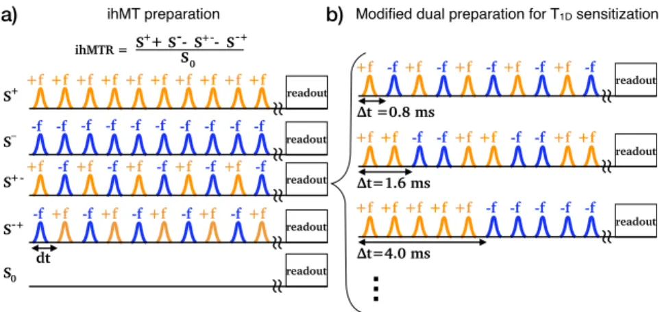
In practice, single-o↵set (S+_{) and dual-o↵set (S}+ _{) MT images can be obtained by applying a train of} shaped RF pulses repeated every dt, prior to the image acquisition. Identical ( = +f ) frequency is applied to all pulses for S+_{, whereas for S}+ _{, an alternation of the frequency from = +f to = f is applied} every other pulse (Fig. 1a). A modification of the dual-o↵set saturation scheme has been proposed to provide additional sensitivity to T1D relaxation [20] and the theoretical ihMT model applied to this modified ihMT sequence enabled the formulation of an analytical solution of the ihMT signal decay as function of T1D and the switching time between positive and negative frequency o↵set pulses. Fits of this analytical solution to experimental data led to rather long T1Ds estimated to _{⇠5-10 ms in myelinated brain tissues (white and} gray matter) and _{⇠15-20 ms in lamellar lipid systems such as hair conditioner [20, 21]. In contrast, other} biological tissues or samples, such as muscle or agarose gels, have shown much shorter dipolar relaxation times (⇠1-3 ms). Long T1Ds in myelinated tissues most likely explain the selective contrast of ihMT images for white matter [22–25] and its high specificity for myelin [26].

The above-presented framework for the dipolar order relaxation time estimation using ihMT MRI sequences relies on a single compartment for T1D. However, recent investigations have suggested that there could be multiple T1D components in myelinated tissues.

Prevost et al. in [21] varied the ihMTR contrast in mouse brain by increasing dt, the repetition time between two consecutive RF pulses in the ihMT preparation (approach called T1Dfiltering). By weighting the ihMT signal towards relatively long T1D, it became clear that short T1D components (T1D_{⌧ dt) would be filtered} out from the MRI signal, enhancing the specificity of ihMT for myelinated tissues. Later on, strategies to optimize the ihMTR values in human brain by alternating bursts of strong RF pulses and a long dead time, while keeping the same global irradiated power, B1RM S, were proposed [27, 28]. These configurations provided a strong sensitivity enhancement and were called boosted ihMT sequences. Duhamel et al. in [26] combined boosted ihMT sequences with various T1D filtering strengths and observed signal variations in brain tissue that were not consistent with the theory if a single T1D component was used to describe myeli-nated tissues, hence suggesting the existence of multiple T1D components in myelin. An alternative view of the T1Ddistribution can be obtained with Jeener-Broekaert measurements [29], which is one of the standard NMR pulse sequences to measure T1D. A rather simple lipid system made of multilamellar vesicles mimicking the lipid composition of myelin was studied by using the Jeener-Broekaert pulse sequence and the results are shown in the Appendix A. The echo time dependence of the Jeener-Broekaert echoes unambiguously shows a multi-exponential feature, hence the existence of multiple T1Ds in lipid membranes. Overall these

evidences led to the belief that multiple T1Ds were also needed for ihMT measurements in myelinated tissues. Previous quantitative models have not considered the e↵ect of multiple components with nonzero T1Don T1D estimation with ihMT. Varma et al. [2] introduced a two-component model of ihMT and MT but assumed one component had zero T1D. In subsequent work [20], when modeling data with modified ihMT preparation including varied frequency switching times, only one T1Dcomponent was modeled using a complicated ana-lytic solution for the ihMT steady state. Herein the model introduced in [20] is called the mono-component T1D model.

In this paper, we propose a general model framework allowing the estimation of multiple T1D components from modified ihMT MRI data. The proposed model was applied with two T1D components and, herein, is called bi-component T1D model. Instead of relying on an analytical solution, a fast matrix formalism was used in order to obtain a closed-form solution of the ihMT signal with minimal approximations. The mono-and bi-component T1Dmodels were compared with regard to fit results and validity of fits over di↵erent RF power regimes for experimental data measured with the modified ihMT sequence in ex-vivo rat spinal cord.

2

Theory

2.1

Dipolar order e↵ects on magnetization transfer MRI

The biophysical model associated with the theory of ihMT with the mono-component T1D is illustrated on Figure 2a, and, following the theory of weak RF saturation in solids developed by Provotorov [17], separates the macromolecular pool of protons into a Zeeman order (↵) and a dipolar order ( ) reservoirs, e↵ectively coupled under the e↵ect of o↵-resonance RF saturation. Using a thermodynamic interpretation of Provotorov theory [18], one can use a system of coupled di↵erential equations to describe the evolution of the spin temperatures of the Zeeman and dipolar reservoirs:

d↵ dt = RRF B(↵ ) R1B(↵ ↵L) d dt = RRF B ✓_2⇡ D ◆2 (↵ ) 1 T1D( L)

in which ↵ and are proportional to the inverse of the Zeeman and dipolar spin temperatures respectively. ↵ = MZB

2⇡ corresponds to the net magnetization of the macromolecular pool initially equal to ↵L = M0B

2⇡ . L ⌧ ↵L can be neglected. RRF B is the RF saturation rate defined by RRF B = ⇡ !21gB(2⇡ ) with !1 the RF power of the RF pulse and gB the normalized absorption lineshape of the macromolecular spins. D corresponds to the local dipolar field expressed in angular frequency unit, and may be calculated from the second moment of gB.

The magnetization exchange between the macromolecular pool and the liquid pool can be further described by the modified Bloch equations such that the equations of evolution for the total spin system, considering only the longitudinal magnetization components, are given by [30, 31]:

dMZA

dt = R1A(M0A MZA) RM0BMZA+ RM0AMZB RRF AMZA dMZB dt = R1B(M0B MZB) RM0AMZB+ RM0BMZA+ 2⇡ RRF B RRF BMZB (1) d dt = 1 T1D + RRF B 2⇡ D2 MZB RRF B ✓_2⇡ D ◆2

with R1A, the relaxation rate of the liquid pool ⇣R1A=_T1A1 ⌘, R1B, the Zeeman relaxation rate of the macromolecular pool⇣R1B = 1

T1B

⌘

, R, the magnetization exchange rate between the macromolecular pool and the liquid pool and RRF A, the RF saturation rate defined by RRF A= ⇡ !2

1gA(2⇡ ).

While single-sided o↵-resonance RF saturation (S+_{) generates dipolar order e↵ects acting against the} satura-tion of the Zeeman order (eq. 1), a symmetric and simultaneous dual-sided o↵-resonance RF saturasatura-tion with equal power applied on positive and negative frequencies (S+ _{) e↵ectively decouples the dipolar order from} Zeeman order thereby cancelling the dipolar order contribution to the MT e↵ects. This is mathematically ver-ified by replacing in eq. 1 the term 2⇡ RRF B= 2⇡ ⇡!2

1gB(2⇡ ) by ⇡2!12gB(2⇡ ) ⇡2!12gB( 2⇡ ), which accounts for halving the RF power between = +f and = f , and which equals zero assuming that the lineshape gB is symmetric [31] gB(2⇡ ) = gB( 2⇡ ). Thus a simple di↵erence of the generated MT images can be computed to make the ihMT image reflecting dipolar order. Then, ihMTR is computed as:

ihM T R = 2S + _S+

S0 , (2)

in which S0 is the unsaturated image.

As mentioned in Varma et al. [2], the di↵erential equations associated with a single T1D component model (Eq. 1) can be straightforwardly extended to take into account several (as indicated by i) Zeeman orders MZBi and dipolar orders i accounting for multi-component T1D model. The bi-component T1D model proposed in this work (Figure 2b) assumes a macromolecular pool divided in a fraction fD associated with a Zeeman order MZB1 coupled to a dipolar order 1and a fraction (1 fD) associated with a Zeeman order MZB2 coupled to a dipolar order 2. Each dipolar order is characterized by its own relaxation time (T1D1 and T1D2). Identical relaxation rate, R1B, and lineshape, gB, are assumed for both components. Finally, the two fractions of macromolecular pool were assumed to exchange with the same rate R with the liquid pool.

2.2

Assessing T

with ihMT

The typical ihMT experiment (Fig. 1a) was modified by Varma et al. [20] to enable T1D measurements (Fig. 1b): the switching time between frequency alternation, t, is increased in a way that multiple pulses are applied with the same frequency before switching to the opposite frequency in the dual-o↵set saturation scheme. By keeping all other sequence parameters (including duty cycle and pulse bandwidth) constant, the modified ihMT signal decays as t increases and as a function of the value of T1D.

For the mono-component T1Dmodel, an analytical solution of equation 1 was found considering the modified ihMT sequence and assuming the steady state condition (eq. 2 and appendix in [20]). This approach allowed for estimation of T1Dfrom ihMT experimental data using conventional least square optimization procedures. To calculate the solution for the bi-component T1D model, we used a matrix representation [32, 33] of equations 4 of Varma et al. [2] to describe the magnetization of each reservoir:

˙

M = AM + B (3)

M = 2 6 6 6 6 6 6 6 4 MZA MZB1 1 MZB2 2 3 7 7 7 7 7 7 7 5 A = 2 6 6 6 6 6 6 4 (R1A+ RM0B+ RRF A) R M0A 0 R M0A 0 R fDM0B (R1B+ RM0A+ RRF B) RRF B2⇡ 0 0 0 RRF B2⇡_D2  1 T1D1+ RRF B ⇣ 2⇡ D ⌘2 0 0 R (1 fD) M0B 0 0 (R1B+ RM0A+ RRF B) RRF B2⇡ 0 0 0 RRF B2⇡_D2  1 T1D2+ RRF B ⇣ 2⇡ D ⌘2 3 7 7 7 7 7 7 5 and B = 2 6 6 6 6 6 6 6 4 R1AM0A R1BfDM0B 0 R1B(1 fD) M0B 0 3 7 7 7 7 7 7 7 5 .

Considering an event of duration t1 in the modified ihMT sequence (i.e. a RF pulse or a relaxation delay) and assuming that A and B are constant during that period of time, a general matrix exponential solution for eq. 3 can be given by equation (6) in [34].

Mt1= e

At1_{Mt=0+ A} 1 _eAt1 _{I B}

The usual power equivalent approximation for rectangular pulses [34, 35] was applied to the used shaped RF pulses to make !1time independent.

Thus, defining P = eAt1 _{and Q = A} 1 _eAt1 _{I B, one can rewrite:}

Mt1 = P Mt=0+ Q

For simplicity, t can be dropped in Mt1 and therefore: M1= P Mt=0+ Q. The matrices P and Q transform

Mt=0 into M1.

Now let us consider a series of events, such as in the case of a train of pulses during the modified ihMT sequence. Consider an initial magnetization Mt=0. Applying a rectangular pulse or a delay can be described by matrices P1 and Q1 such that M1 = P1Mt=0+ Q1. Then the successive events are described by the following equations:

t = t0 Mt=0

t = t1 M1= P1Mt=0+ Q1

t = t3 M3= P3M2+ Q3= P3P2P1Mt=0+ P3P2Q1+ P3Q2+ Q3 t = t4 M4= P4M3+ Q4= P4P3P2P1Mt=0+ P4P3P2Q1+ P4P3Q2+ P4Q3+ Q4 ... t = tN MN = PNMN 1+ QN = PNeqMt=0+ Q eq N, in which PNeq and Q eq

N are the equivalent matrices of applying all the N events:

P_Neq= N Y i=1 Pi QeqN = N X j=1 2 6 6 4 0 B B @ N Y i=j+1 j<N Pi 1 C C A Qj 3 7 7 5

in whichQis the leftwise product operator.

The steady state solution for the modified ihMT sequence is then found by imposing that Mt=0 = MN, in which N is the number of events corresponding to the periodicity of the RF saturation scheme (i.e. t for single o↵set saturation and 2 t for dual o↵set saturation):

MSS = (I PNeq) 1

QeqN

The assumption of steady state is not necessary but was chosen to reduce the computation time of simulations and data fits. Define P+, Q+ the matrices P and Q for a RF pulse with a positive o↵set frequency; P , Q likewise; Pr, Qr the matrices corresponding to a relaxation during the delay between two pulses. The magnetization in the steady state after the single saturation S+ is:

S+= (I PrP+) 1(PrQ++ Qr)

Likewise, the magnetization in the steady state after the dual saturation S+ _{is (given n} 2 N⇤_): S+ ( t = n dt) = [I (PrP )n(PrP+)n] 1 ( (PrP )n "_{n 1} X i=0 (PrP+)i # (PrQ++ Qr) + "_{n 1} X i=0 (PrP )i # (PrQ + Qr) ) Then ihM T R( t) = 2S + _S+ _{( t)} S0 . (4)

Therefore, ihMTR in the steady state can be simulated for each t value. Conversely, one can also estimate T1D1, T1D2and fD (or other parameters) given ihMTR( t) data by using optimization algorithms such as non-linear least squares.

3

Methods

3.1

Ethics statement

Experiments were conducted on a fixed rat spinal cord and were performed following French guidelines for an-imal care from the French Department of Agriculture (Anan-imal Rights Division), the directive 2010/63/EU of the European Parliament and of the Council of 22 September 2010 and approved by our institutional commit-tee on Ethics in animal research (Comit´e d’´Ethique de Marseille n 14, project authorization APAFIS#1747-2015062215062372v6).

3.2

MRI measurements

Ex-vivo modified ihMT measurements were performed on a Bruker Pharmascan 7T with a volume emitter coil and a 4-element array receiver cryoprobe on an excised, fixed rat spinal cord (cervical level) immersed in normal phosphate bu↵ered saline (PBS) maintained at 40_{±1 C during all the experiment. Enough time} was waited before the acquisition until the spinal cord presented a stable S0 image, indicating that the temperature was approximately constant. The modified ihMT preparation (Fig. 1b) consisted of 2000 pulses of 0.5 ms with a delay of 0.3 ms between each pulse. The total saturation time was 1.6 s. The o↵set frequencies were 9700 Hz and -10300 Hz (that is slightly o↵-centered with respect to the free water resonance line to compensate for the chemical shift of the macromolecular line [36]). The switching time, t, was set to each of the values: 0.8; 1.6; 4; 8; 16; 20 ms. The root mean square power calculated over the total ihMT preparation, B1RM S was set to each of the values 3.5; 5.8; 6.7; 8.0; 9.0 µT. The ihMT preparation was followed by a single slice single-shot RARE (rapid acquisition with relaxation enhancement) readout module with echo time 2.978 ms, e↵ective echo time 23.80 ms, RARE factor = 71, partial Fourier acceleration = 1.8, FOV 20 mm x 20 mm, matrix size 128 x 128 voxels, slice thickness 4 mm. The number of averages for each individual MT contrast (single-o↵sets and dual-o↵sets) was 150 for each t and B1RM S values. The acquisition time was about 20 hours for the whole dataset.

3.3

Fitting T

T1D maps of rat spinal cord were generated by voxelwise fitting of the solutions of the mono- and bi-component T1D models to the ihMTR( t) images. Matlab (The MathWorks Inc., Natick, MA) was used, specifically the built-in function lsqcurvef it, a nonlinear least-squares solver. For the mono-component T1D model, the analytical solution as presented in Varma et al. [20] was used to derive T1Dand A maps, in which A is a normalization factor and is equivalent to 0.5ihMTR( t = 0). For the bi-component T1D model, the solution derived from the matrix exponential approach (eq. 4) was used to extract T1D1, T1D2, fD (and 1 fD). Considering the sensitivity analyses in Varma et al. [20], which showed that ihMT is more sensitive to T1D and less sensitive to other MT parameters when using the experimental framework of modified ihMT sequence, the following fixed parameter values [20] were used for both models: R = 26 s 1_{, RM}B

0 /R1A = 2.3, 1/(R1AT2A) = 22, T2B = 9.7 µs, R1B = 1 s 1_{, R1A = (1.8)} 1 _s 1_.

In order to assess the validity of the fits, Bayesian Information Criterion (BIC) and residual variance (resVar) were employed [37]. BIC is defined as [37]:

BIC = p ln(n) 2 ln(L),

in which p is the number of parameters to be fit and ln(L) is the maximum log-likelihood of the estimated model. For a nonlinear fit with normally distributed errors [37]:

ln(L) = 0.5 n ln 2⇡ + 1 ln n + ln n X i=1 x2i !! ,

in which xi are the residuals from the fit and n is the number of data points.

Such index promotes data fidelity (i.e. minimum residual sum of squares) and model parsimony (minimal number of model parameters) at the same time. In this sense, the best model is the one that minimizes BIC. The residual variance is defined as [37]:

resV ar = Pn

i=1x2i n p .

It quantifies the amount of variance that is not taken into account by the model. The residual variance was used only to compare two models, in the form of a ratio of their values (ratio bi : mono-component

T1D). Assessing the residual variance ratio allows comparing di↵erent fitting models accounting for di↵erent degrees of freedom. In this case, the smaller the ratio is, the more advantageous the bi-component T1Dmodel. Regions of interest (ROI) in the white matter (WM) and gray matter (GM) of the spinal cord were manually delineated in the ihMTR images (Fig. 3) and reported to the T1D, A and T1D1, T1D2, fD, (1 fD) maps. Mean and standard deviation values of T1D, A and T1D1, T1D2, fD, (1 fD) were then calculated in these ROIs.

4

Results

4.1

MRI measurements

A set of ihMTR images was obtained for each combination of t and B1RM S values. Figure 3 shows the ihMTR( t) images acquired with B1RM S = 6.7 µT. A strong white versus gray matter contrast is achieved with a clear delineation of the gray matter “butterfly” shape within the cord. One can clearly observe the ihMTR attenuation as t increases as a consequence of varying T1D weighting.

4.2

Mono-component T

model fits

Figure 4a shows T1D and A maps obtained by voxelwise fitting the analytical solution for the mono-component T1D model to the ihMTR( t) data. All maps have the same field of view. Figure 4b shows bar plots of the T1D and A values for white and gray matter for each B1RM S. The BIC values are listed in Table 2 (Appendix B).

A values, which highly correlate with ihMTR, resulted in A maps sharper than T1D maps. T1D maps are noisier, with somewhat high values in the ihMTR signal-free area. Hence, both maps must be interpreted together: T1Dassociated with low values of A should not be considered relevant.

Results presented in Figure 4 show that white matter consistently has a longer apparent T1D than gray mat-ter, leading to a relative T1D contrast between the two structures defined as (T1DW M T1DGM)/T1DW M of⇠0.17 at B1RM S=3.5 µT and increasing up to_{⇠0.25 at B}1RM S=9 µT. Additionally, the estimated T1D values in both WM and GM decrease with B1RM S whereas the scaling factor A, proportional to ihMTR( t = 0), greatly increases.

4.3

Bi-component T

fits

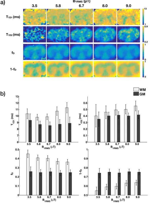
Matrix exponential solution of the bi-component T1D model (Eq. 4) was used to fit voxelwise the same set of modified ihMTR( t) images of the spinal cord (Fig. 3). Figure 5a shows maps of T1D1, T1D2, fD and (1 fD). All maps have the same field of view. Figure 5b shows the bar plots of T1D1, T1D2, fDand (1 fD) values for white and gray matter for each B1RM S. The BIC values obtained for the bi-component T1Dmodel are listed in Table 3 (Appendix B).

Overall, for white matter, long T1D(T1D1) on the order of 10 ms [9.8-11.3 ms] and short T1D (T1D2) on the order of 500 µs [403-555 µs] were found. Both T1D1 and T1D2 were consistently shorter in the gray matter; T1D1_{⇠9ms [8.5-9.3 ms] and T}1D2⇠400 µs [354-418 µs]. The fraction of long T1Dcomponents, fD, was greater in white matter compared to gray matter (conversely, 1 fD is greater in gray matter). In white matter, (1 fD) increases with B1RM S, consistent with the more important contribution of short T1Dcomponents as B1RM S increases. Likewise, the maps of the short T1Dcomponent (T1D2) look less noisy as B1RM Sincreases.

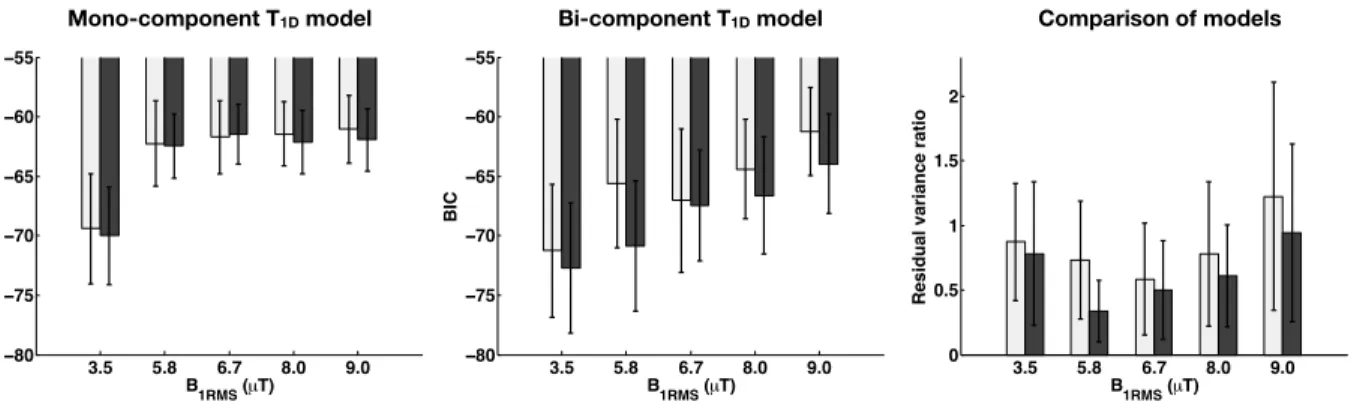
Figure 6 includes the bar graphs of BICs of each model and the residual variance ratio, for each RF power. Based on the BIC and residual variance ratio statistics, one can observe that the proposed bi-component T1D model improves the fits (lower BIC values, and residual variance ratio <1), with best relative improvement for 5.8-8.0 µT. For the lowest (B1RM S=3.5 µT) and the highest (B1RM S=9.0 µT) saturation powers, BIC and residual variance ratio statistics indicate moderate, if no improvement with the proposed bi-component T1D model.

5

Discussion

5.1

Multiple T

s in myelinated tissues

Since T1D is a tissue property that should be una↵ected by B1RM S, the decrease of T1Ds derived from the mono-component T1D model as B1RM S increases (Fig. 4) suggest that a refinement of the tissue model is required. It is also consistent with the hypothesis that spinal cord would have di↵erent components with distinguishable T1Ds contributing to the ihMT signal: the mono-component T1D model would actually per-ceive an apparent T1D which depends on how much the short T1D component is observed given the RF power. This hypothesis was further supported by simulations performed on synthetic data generated with the proposed bi-component T1D model with short and long T1Ds, and then fit using the mono-component T1D model (see Supplementary Material).

Multiple T1Ds imply that the hypothesis of a single dipolar spin temperature is not fulfilled within such spin systems, suggesting that spin di↵usion or other exchange processes are not fast enough to average the macromolecular pool magnetization in a single e↵ective pool. There are several possible explanations for the presence of multiple T1Ds in myelinated tissues. One is that myelin lipids could have a heterogeneous molecular mobility with several proton populations experiencing various kinds of molecular motions in terms of frequency (or correlation time) and intensity. These may correspond to di↵erent segmental motions along the phospholipid chain [38, 39]. Hence, dipolar order would relax in a multi-exponential fashion, as found with the NMR Jeener-Broekaert experiments on multilamellar vesicles of lipids (see Appendix A). Another possible explanation would simply be that each T1D component actually corresponds to di↵erent molecular assembly, either arising from other chemical environments rather than fatty acid chains, or from other struc-tures rather than myelin itself located in the same voxel.

Of importance, this work demonstrates that the framework combining the ihMT model with two T1Ds, a matrix exponential approach to solve ihMTR and a modified ihMT experiment is a viable MRI approach for multi-component T1D mapping. It allowed estimating short T1Don the order of 500 µs and long T1Don the order of 10 ms in fixed spinal cord white matter. In terms of quantitative values, this result could be compared with those obtained on the synthetic membrane lipid system with NMR Jeener-Broekaert analysis (see Appendix A), which suggests the existence of several components, in the sub-millisecond range, 10 ms range and over 100 ms range. The T1Dvalues obtained in this study are also in close agreement with results obtained by Eliav et al. [39], who, by using a NMR sequence that combines double and zero quantum filters with magnetization transfer, measured a tri-exponential decay of the dipolar order in porcine spinal cord, with T1Dvalues of 0.11, 0.86 and 11.4 ms. Understanding the physico-chemical origins of these components is of great importance to interpret further in vivo ihMT data, however, this is outside the scope of the current study, and will require a stronger focus on in vitro and ex vivo NMR experiments.

Our results with the bi-component T1Dmodel suggest that the short T1D component only measurably con-tributes to ihMT for powers 5.8 µT (Fig. 5a). Not only the T1D2 maps become less noisy as B1RM S increases, but also the fraction associated with short T1D, (1 fD), increases, reaching up to 60% for white matter, while stable at >70% for gray matter. These findings are consistent with the condition for dipolar or-der to contribute to ihMT signal, given by RRF BT1D> 0.01 [4]. For example, assuming a Super-Lorentzian

lineshape, the RRF B values at 10 kHz for 3.5, 5.8, 6.7, 8.0 and 9.0 µT are, respectively: 9.7, 26.1, 35.4, 50.5 and 63.6 s 1_{, allowing observable T1Dhigher than: 1.03, 0.38, 0.28, 0.20, 0.16 ms, respectively. However, one} must consider that the contribution from very short T1Ds is attenuated by the T1Dfiltering that occurs even with the shortest value of t (or dt). Due to hardware limitations, as well as the fact that the bandwidth of short pulses needs to remain relatively narrow to prevent direct saturation of the free pool, the dt used in this work was 0.8 ms, which does not allow efficient sampling of very short T1Dcomponents (T1D_{⌧ 0.8 ms).} Comparison of residual variance ratio across fits suggests further insights into the T1Dcomponents in tissue (Fig. 6). Low RF power (B1RM S=3.5 µT) led to similar residuals for both models, indicating that the bi-component T1D model does not perform much better than the mono-component T1D model most likely because short T1D components weakly contribute to the ihMT signal at such power level. Hence, this con-firms that the mono-component T1D model used in Varma et al. [20] to estimate T1D is reasonable for the powers achievable in-vivo in humans. For the [5.8-8.0 µT] range, the small residual variance ratios (Fig. 6) and the lower BIC values for bi-component T1D model indicate that the proposed bi-component model is more appropriate to fit the data. Interestingly, for 9.0 µT, larger residual variance ratios indicate reduced performance of both models in that power regime. This potentially implies that a model with a higher num-ber of components would be required to more precisely describe the distribution of short T1Din the system as B1RM S is increased. Noteworthy, including a third T1D component in the model is straight-forward from a mathematical point of view; but as new parameters are included in the model, the number of required experimental data points to estimate all model parameters should be higher. In addition, the SNR needed to correctly estimate them increases, as well as the computation time of the fitting. In the current work we limited our e↵ort to the bi-component T1D model for these reasons.

5.2

White matter / gray matter T

contrast

Our results showed significantly di↵erent T1Ds in white and gray matter, indicating sensitivity of T1D for tissue composition and di↵erent myelin organizations. Swanson et al. [3] found T1Dof 11.1±1.8 ms in white matter and 4.06±1.20 ms in gray matter (bovine spinal cord ex-vivo at 40 C), by using a mono-exponential fit on the Jeener-Broekaert echoes considering values of ⌧ greater than 600 µs. On the other hand, Varma et al. [20] found a reduced di↵erence between white and gray matter: 6.0_{±0.5 ms for posterior white matter} and 5.9_{±1.2 ms for posterior gray matter (human brain in-vivo; B}1RM S=3.5 µT and physiological temper-ature, see Table 3 in [20]), by using the mono-component T1D model of ihMT. These three sets of results are not necessarily contradictory: they were performed in di↵erent specimen, temperature and interpreted with di↵erent models. The experiments in [20] used a relatively low B1RM S, 3.5 µT, which was probably not enough to exploit the contribution of short T1D components in gray matter, so the apparent T1D reported by Varma et al. [20] in white and gray matter seemed about the same.

5.3

In vivo multiple T

measurement?

Good T1D maps require ihMTR images with high SNR. In our studies, the SNR for B1RM S=6.7 µT and t=0.8 ms was 277. This SNR level was reached with a slice thickness of 4.0 mm, spatial resolution of 0.156 mm/voxel and 150 repetitions per B1RM S and per t. Besides, the number of ts acquired must be large enough to estimate all the three parameters (T1D1, T1D2 and fD). In this study, good fits were obtained with six values of t, spanning from 0.8 to 20 ms. These constrains and requirements can be a limitation for in-vivo studies as the time needed to acquire a full set of ihMTR( t) data was about 20 hours. However, there is room for improvement. For instance, currently, the single saturation images, S+ _{and S (Fig. 1),} are acquired as many times as the dual saturation images, S+ _{( t) and S} +_{( t), while S}+ _{and S are the} same for every t.

The dependence of apparent T1D on power has been demonstrated in this work, and yielded important knowledge on how the ihMT signal is generated and filtered, all consistent with the dipolar order theory. Currently, clinical investigations of ihMT are typically performed at either 1.5T or 3T [40], which can deliver B1RM S around 4µT and 2µT , respectively. Whereas the RF power may reach higher levels during the sat-uration periods [27, 28], one has to keep these orders of magnitude in mind when interpreting in vivo ihMT data and associate them with putative T1D values.

Furthermore, the T1Dvalues found in this work could di↵er from the values we could expect in vivo, because of the spinal cord fixation. Crosslinking tissue proteins with formaldehyde could alter the motional spectral densities and therefore a↵ects T1D values.

5.4

Limitations

This work demonstrates the feasibility of interpreting ihMT images with at least two non-zero T1D, and provided an order of magnitude for the short and long T1Dvalues, 500 µs and 10 ms respectively. It did not intend to provide reference values of T1D in spinal cord white and gray matter. This focus would require a higher number of specimens and validation of the T1D values derived from ihMT. This could be obtained by the comparison of T1D values measured with the Jeener-Broaekaert sequence and the modified-ihMT sequence on the same lipid systems and in the same experimental conditions.

Only two components (short and long T1D) were considered in the proposed model. Assessment of a third very short T1D, such as the one found by Eliav et al. [39], 0.11 ms, is limited by the experimental setup. The use of shorter RF pulses would be needed, however the direct saturation caused by short pulses should be avoided.

The fixed parameters (R, RMB

0 /R1A, 1/(R1AT2A), T2B, T1B, R1A) enabled a fast, simple demonstration of the proposed model. This work did not aim to evaluate the influence of these parameters on the T1Doutput. Furthermore, the assumption that both dipolar reservoirs have the same lineshape (thus T2B) and same exchange rate R is a simplification, since we could not distinguish these values without further investigation of the origins of multiple dipolar reservoirs.

Finally, in this work we fit only the ihMTR( t) values, not the MT values. This approach was chosen because we were concerned about the ihMT parameters only. On the other hand, this means that the values found for fD are only relative to the two components contributing to ihMT. Therefore, comparisons with qMT fits [35] in the literature may be avoided.

6

Conclusion

A bi-component T1D model was proposed and better interpreted the behavior of ihMT signal acquired with the modified ihMT sequence under di↵erent RF saturation powers compared to the mono-component T1D model. It allows measuring short and long T1D (on the order of 500 µs and 10 ms, respectively) in spinal cord tissue. Although a theory that would relate T1D values to biological membrane properties, such as fluidity and elasticity, is still required, this work is an important step in the demonstration that ihMT MRI could be an interesting tool for in vivo membrane characterization.

7

Acknowledgements

This project has received funding from the European Union’s Horizon 2020 research and innovation pro-gramme under the Marie Sk lodowska-Curie grant agreement N 713750. Also, it has been carried out with

S+

-S+

ihMT preparation Modified dual preparation for T1D sensitization

…

~

~

~

~

~

~

~

~

~

~

~

~

~

~

~

~

Figure 1: ihMT MRI sequence. a) ihMT preparation including single-o↵set and dual-symmetric o↵set saturations. b) Modified ihMT sequence introduced by Varma et al. [20]. In practice, the single-sided o↵-resonance RF saturation MT image is computed from the average of a MT image obtained with a positive o↵set (S+_{) and one with a negative o↵set (S ) in order to correct for first order asymmetry e↵ects of} gB arising from the chemical shift of the broad macromolecular lines [36]. For signal-to-noise ratio (SNR) purpose, the dual-sided o↵-resonance RF saturation is also repeated twice, changing the sign of o↵set of the pulse (S+ _{and S} +_).

the financial support of the Regional Council of Provence-Alpes-Cˆote d’Azur and with the financial support of the A*MIDEX (n ANR- 11-IDEX-0001-02), funded by the Investissements d’Avenir project funded by the French Government, managed by the French National Research Agency (ANR).

Liquid pool Zeeman Order Macromolecular pool Dipolar Order Zeeman Order

T

f

T

1-f

T

f

=1

a)

b)

Figure 2: A) Mono-component T1D ihMT model presented in [20]. B) Proposed bi-component T1D ihMT model. ihMT ratio (0− 10%) 0 1 2 3 4 5 6 7 8 9 10 0 11% Δt = 0.8 ms Δt = 1.6 ms Δt = 4.0 ms Δt = 8.0 ms Δt = 16.0 ms Δt = 20.0 ms WM GM

Figure 3: Representative ihMT rat spinal cord images. Left: anatomical T2-weighted image of the rat spinal cord. Middle: ihMTR images acquired with increasing t (B1RM S=6.7 µT). Right: Regions of interest (ROI) selected for quantitative analyses in white and gray matter.

T1D (ms) A (%) 3.5 5.8 6.7 8.0 9.0 B1RMS (μT) 1 13 0 7

a)

b)

Figure 4: Mono-component T1D model outcomes. a) T1D (upper row) and scaling factor A (lower row) maps of rat spinal cord derived by fitting the analytical solution for the mono-component T1D model [20] to ihMTR( t) (Fig. 3). b) Bar plots of T1D (left) and A (right) values measured in ROIs selected in white (WM) and gray matter (GM) (Fig. 3) for di↵erent B1RM S.

T1D1 (ms) 3.5 5.8 6.7 8.0 9.0 B1RMS (μT) 1-fD 1 13 0 1 T1D2 (ms) 0.2 0.9 0 1 fD

a)

b)

Figure 5: Bi-component T1D model outcomes. a) T1D1, T1D2, fD, and (1 fD) maps of rat spinal cord obtained by using the proposed bi-component T1DihMT model. b) Bar plots of T1D1, T1D2, fDand (1 fD) values measured in ROIs selected in white (WM) and gray matter (GM) (Fig. 3) for di↵erent B1RM S.

3.5 5.8 6.7 8.0 9.0 −80 −75 −70 −65 −60 −55 BIC B_1RMS (µT) 3.5 5.8 6.7 8.0 9.0 −80 −75 −70 −65 −60 −55 BIC B_1RMS (µT)

Mono-component T1D model Bi-component T1D model Comparison of models

3.5 5.8 6.7 8.0 9.0 0 0.5 1 1.5 2

Residual variance ratio

B_1RMS (µT)

Figure 6: BIC values of each model fit: mono-component (left) and bi-component (middle). Residual variance ratio (bi : mono-component T1D models) for gray and white matter for each B1RM S (right). Values less than one indicate a better performance of the proposed model.

8

Appendix A: NMR Study

8.1

Synthetic membrane preparation

Lipids were purchased from Avanti Polar Lipids, Inc. (Alabaster, Alabama, USA): 1-palmitoyl-2-oleoyl-sn-glycero-3-phosphocholine (POPC), total cerebrosides (brain, porcine) and cholesterol (ovine). Multilamellar vesicles (MLV) of lipids were made by the following steps [41]:

• Appropriate amounts of lipids were weighed to obtain the proportions POPC: 40%; cholesterol 40%; cerebrosides 20% (molar ratio).

• The lipids were dissolved in organic solvent (CHCl3), the solvent was evaporated, water was added, and the sample was shaken in a vortex mixer and lyophilized overnight to remove solvent traces. • A suitable volume of heavy water, D2O, was added to obtain a lipid hydration of 80% (v/w). Hydration

is defined as the mass of water over the total mass of the system (phospholipids and water).

• The hydrated sample was then vigorously shaken in a vortex mixer, frozen in liquid nitrogen, and heated to 37 C for 10 min in a water bath. This cycle of liposome (multilamellar vesicles) formation was repeated three times until a milky dispersion was obtained at room temperature.

• The resulting dispersion was transferred into a 4-mm NMR ZrO2 rotor (100 µl) that was placed in the magnetic field.

8.2

NMR measurements

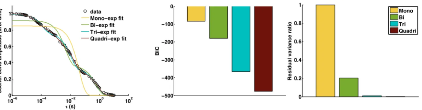
The NMR measurements were performed on a Bruker Avance III 500 MHz spectrometer by means of a dual resonance1_H/15_N-31_{P broad band 4mm CPMAS probe, with a Jeener-Broekaert pulse sequence [29],} a standard NMR method to measure T1D. This sequence consists of one 90 pulse followed by two 45 pulses: 90 ( 1)-t-45 ( 2)-⌧ -45 ( 3)-acq( 4). The RF and receiver phase cycling was used as in [3] in order to eliminate multiple quantum and Zeeman order magnetization during ⌧ . The length of the 90 -pulse was 2.62 µs, t was set to 30 µs and ⌧ was set to 64 values from 1 µs to 10 s. The spectral width was 150 kHz and 32768 points were acquired for each ⌧ . The number of scans was 40. Data were obtained at 312 K. The decay of the maximum absolute value of the Jeener echoes was fit with di↵erent exponential models: mono, bi, tri and quadri-exponential.

100−6 10−4 10−2 100 102 0.2 0.4 0.6 0.8 1 τ (s)

Jeener echo amplitude (arb. unit)

data Mono−exp fit Bi−exp fit Tri−exp fit Quadri−exp fit −500 −400 −300 −200 −100 0 BIC 0 0.2 0.4 0.6 0.8 1

Residual variance ratio

Mono Bi Tri Quadri

Figure 7: (left) Jeener-Broekaert echo decays in a synthetic membrane (POPC: 40%; cholesterol 40%; cere-brosides 20% (molar ratio)) and fitted with multi-exponential models. (midlle) BIC values of each exponential model fit. (right) Residual variance ratio between each exponential model and the mono-exponential model.

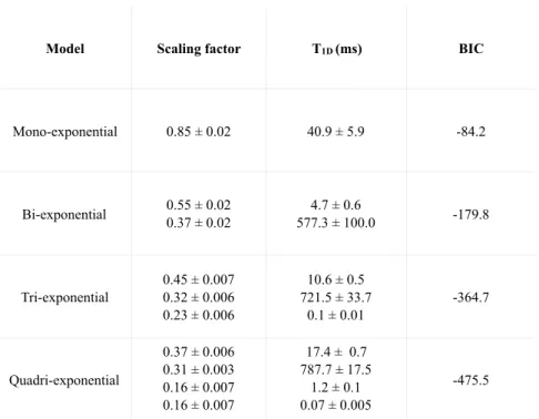
The decay of the Jeener echoes with ⌧ , the delay after the second pulse, in this membrane unambiguously shows multi-exponential features. Figure 7 shows that the data points are poorly fit with a mono-exponential model, while bi-, tri-, quadri-exponential fits provide better results (lower BIC values). The T1D values es-timated from these fits are listed in Table 1. Although the accuracy of the quadri-exponential fit might be questionable, one can infer that a single T1D is not enough to describe the dipolar relaxation in this membrane. These results suggest that the ihMT model to assess T1D in complex lipid membranes such as myelin should also consider more than one dipolar component.

Model Scaling factor T1D (ms) BIC Mono-exponential 0.85 ± 0.02 40.9 ± 5.9 -84.2 Bi-exponential 0.55 ± 0.02 _{0.37 ± 0.02 577.3 ± 100.0}4.7 ± 0.6 -179.8 Tri-exponential 0.45 ± 0.007 0.32 ± 0.006 0.23 ± 0.006 10.6 ± 0.5 721.5 ± 33.7 0.1 ± 0.01 -364.7 Quadri-exponential 0.37 ± 0.006 0.31 ± 0.003 0.16 ± 0.007 0.16 ± 0.007 17.4 ± 0.7 787.7 ± 17.5 1.2 ± 0.1 0.07 ± 0.005 -475.5

Table 1: Outcomes of multi-exponential Jeener-Broekaert echo fits obtained on a synthetic membrane (POPC: 40%; cholesterol 40%; cerebrosides 20% (molar ratio)).

9

Appendix B: Tables of fits

Table 2 lists the quantitative mean values of T1D, the scaling factor, A, and the BIC values in white and gray matter, for the fits using the mono-component model. Table 3 lists all the fit results using the proposed bi-component model, as well as the BIC scores in white and gray matter, for each B1RM S.

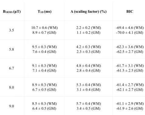
B1RMS (µT) T1D (ms) A (scaling factor) (%) BIC 3.5 10.7 ± 0.6 (WM)
 8.9 ± 0.7 (GM) 2.2 ± 0.2 (WM)
 1.1 ± 0.2 (GM) -69.4 ± 4.6 (WM)
 -70.0 ± 4.1 (GM) 5.8 9.5 ± 0.3 (WM) 7.6 ± 0.4 (GM) 4.2 ± 0.3 (WM)
 2.3 ± 0.3 (GM) -62.3 ± 3.6 (WM)
 -62.5 ± 2.7 (GM) 6.7 9.1 ± 0.3 (WM)
 7.1 ± 0.4 (GM) 4.8 ± 0.4 (WM)
 2.8 ± 0.4 (GM) -61.7 ± 3.1 (WM)
 -61.5 ± 2.5 (GM) 8.0 8.9 ± 0.3 (WM) 6.7 ± 0.5 (GM) 5.3 ± 0.4 (WM)
 3.1 ± 0.4 (GM) -61.4 ± 2.7 (WM)
 -62.1 ± 2.7 (GM) 9.0 8.5 ± 0.3 (WM) 6.4 ± 0.5 (GM) 5.7 ± 0.4 (WM)
 3.4 ± 0.5 (GM) -61.1 ± 2.9 (WM)
 -61.9 ± 2.6 (GM)

Table 2: Mean and standard deviation values of T1Dand A values, as well as BIC values, in rat spinal cord white (WM) and gray matter (GM), obtained by fitting of the analytical solution for the mono-component T1D model to experimental ihMTR( t) data for di↵erent B1RM S.

B1RMS (µT) T1D1 (ms) T1D2 (µs) fD 1-fD BIC 3.5 10.3 ± 0.8 (WM) _{9.3 ± 1.0 (GM)} 403 ± 173 (WM) _{354 ± 110 (GM)} 0.5 ± 0.04 (WM) _{0.3 ± 0.05 (GM)} 0.5 ± 0.04 (WM) _{0.7 ± 0.05 (GM)} -71.3 ± 5.6 (WM) _{-72.7 ± 5.5 (GM)} 5.8 9.8 ± 0.4 (WM) _{8.7 ± 0.5 (GM)} 458 ± 98 (WM) _{403 ± 57 (GM)} 0.4 ± 0.03 (WM)
_{0.2 ± 0.03 (GM)} 0.6 ± 0.03 (WM)
_{0.8 ± 0.03 (GM)} -65.6 ± 5.4 (WM)
_{-70.9 ± 5.5 (GM)} 6.7 9.9 ± 0.4 (WM) _{8.5 ± 0.6 (GM)} 494 ± 81 (WM)
_{412 ± 54 (GM)} 0.4 ± 0.03 (WM) _{0.3 ± 0.04 (GM)} 0.6 ± 0.03 (WM) _{0.7 ± 0.04 (GM)} -67.0 ± 6.0 (WM) _{-67.4 ± 4.7 (GM)} 8.0 10.8 ± 0.7 (WM) _{8.7 ± 0.7 (GM)} 503 ± 71 (WM) _{400 ± 47 (GM)} 0.4 ± 0.03 (WM) _{0.2 ± 0.03 (GM)} 0.6 ± 0.03 (WM) _{0.8 ± 0.03 (GM)} -64.4 ± 4.2 (WM) _{-66.6 ± 4.9 (GM)} 9.0 11.3 ± 0.8 (WM) _{8.9 ± 1.0 (GM)} 555 ± 76 (WM) _{418 ± 61 (GM)} 0.4 ± 0.03 (WM) _{0.2 ± 0.03 (GM)} 0.6 ± 0.03 (WM) _{0.8 ± 0.03 (GM)} -61.2 ± 3.7 (WM) _{-64.0 ± 4.2 (GM)}

Table 3: Mean and standard deviation values of T1D1, T1D2, fD and 1 fD, as well as BIC values, for di↵erent B1RM S, in rat spinal cord white (WM) and gray matter (GM), obtained by using the proposed model.

References

[1] G. Varma, G. Duhamel, C. de Bazelaire, and D. C. Alsop. Magnetization transfer from inhomo-geneously broadened lines: A potential marker for myelin. Magn. Reson. Med., 73:614–622, 2015. doi:10.1002/mrm.25174.

[2] G. Varma, O.M. Girard, V.H. Prevost, A.K. Grant, G. Duhamel, and D.C. Alsop. Interpretation of magnetization transfer from inhomogeneously broadened lines (ihMT) in tissues as a dipolar or-der e↵ect within motion restricted molecules. Journal of Magnetic Resonance, 260:67–76, 2015. https://doi.org/10.1016/j.jmr.2015.08.024.

[3] S. D. Swanson, D. I. Malyarenko, M. L. Fabiilli, R. C. Welsh, J. Nielsen, and A. Srinivasan. Molecular, dynamic, and structural origin of inhomogeneous magnetization transfer in lipid membranes. Magn. Reson. Med., 77:1318–1328, 2016. doi:10.1002/mrm.26210.

[4] A. P. Manning, K. L. Chang, A. L. MacKay, and C. A. Michal. The physical mechanism of “in-homogeneous” magnetization transfer MRI. Journal of Magnetic Resonance, 274:125–136, 2017. http://dx.doi.org/10.1016/j.jmr.2016.11.013.

[5] Ronald Y. Dong. Relaxation and the dynamics of molecules in the liquid crystalline phases. Progress in Nuclear Magnetic Resonance Spectroscopy, 41(1):115 – 151, 2002.

[6] R. C. Zamar, E. Anoardo, O. Mensio, D. J. Pusiol, S. Becker, and F. Noack. Order fluctuations of the director in nematic thermotropic liquid crystals studied by nuclear magnetic resonance dipolar relaxation. The Journal of Chemical Physics, 109(3):1120–1124, 1998.

[7] Takahiro Ueda, Sadamu Takeda, Nobuo Nakamura, and Hideaki Chihara. Molecular motion and phase changes in long chain solid normal alkanes as studied by 1H and 13C NMR. Bulletin of the Chemical Society of Japan, 64(4):1299–1304, 1991.

[8] Lucia Calucci and Claudia Forte. Proton longitudinal relaxation coupling in dynamically heterogeneous soft systems. Progress in Nuclear Magnetic Resonance Spectroscopy, 55(4):296–323, 2009.

[9] E.J. Dufourc, C. Mayer, J. Stohrer, G. Altho↵, and G. Kothe. Dynamics of phosphate head groups in biomembranes. Comprehensive analysis using phosphorus-31 nuclear magnetic resonance lineshape and relaxation time measurements. Biophysical Journal, 61(1):42–57, 1992. https://doi.org/10.1016/S0006-3495(92)81814-3.

[10] T. R. Molugu, S. Lee, and M. F. Brown. Concepts and methods of solid-state NMR spectroscopy applied to biomembranes. Chemical Reviews, 117(19):12087–12132, 10 2017. doi:10.1021/acs.chemrev.6b00619. [11] R Van Steenwinkel. The spin lattice relaxation of the nuclear dipolar energy in some organic crystals

with slow molecular motions. Zeitschrift f¨ur Naturforschung A, 24(10):1526–1531, 1969.

[12] O Lauer, D Stehlik, and K.H Hausser. Nuclear zeeman and dipolar relaxation due to slow motion in aromatic single crystals. Journal of Magnetic Resonance (1969), 6(4):524 – 532, 1972.

[13] R. Gaspar, E.R. Andrew, D.J. Bryant, and E.M. Cashell. Dipolar relaxation and slow molecular mo-tions in solid proteins. Chemical Physics Letters, 86(4):327 – 330, 1982. https://doi.org/10.1016/0009-2614(82)83516-1.

[14] O. Mensio, R.C. Zamar, F. Casanova, D.J. Pusiol, and R.Y. Dong. Intramolecular character of the intrapair dipolar order relaxation in the methyl deuterated nematic para-azoxyanisole. Chemical Physics Letters, 356(5–6):457 – 461, 2002. http://dx.doi.org/10.1016/S0009-2614(02)00347-0.

[16] B. Ohler, K. Graf, R. Bragg, T. Lemons, R. Coe, C. Genain, J. Israelachvili, and C. Husted. Role of lipid interactions in autoimmune demyelination. Biochimica et Biophysica Acta (BBA) - Molecular Basis of Disease, 1688:10 – 17, 2004. https://doi.org/10.1016/j.bbadis.2003.10.001.

[17] B. N. Provotorov. Magnetic resonance saturation in crystals. Sov. Phys. JETP, 14(5):1126–1131, 1962. [18] M. Goldman. Spin temperature and nuclear magnetic resonance in solids. International series of

mono-graphs on physics. Oxford: Clarendon Press, 1970.

[19] J.-S. Lee, A. K. Khitrin, R. R. Regatte, and A. Jerschow. Uniform saturation of a strongly coupled spin system by two-frequency irradiation. J. Chem. Phys., 134, 234504, 2011. doi:10.1063/1.3600758. [20] G. Varma, O. M. Girard, V. H. Prevost, A. K. Grant, G. Duhamel, and D. C. Alsop. In vivo measurement

of a new source of contrast, the dipolar relaxation time, T1D, using a modified inhomogeneous magne-tization transfer (ihMT) sequence. Magn. Reson. Med., 78:1362–1372, 2017. doi:10.1002/mrm.26523. [21] V.H. Prevost, O.M. Girard, S. Mchinda, G. Varma, D.C. Alsop, and G. Duhamel. Optimization of

inho-mogeneous magnetization transfer (ihMT) MRI contrast for preclinical studies using dipolar relaxation time (T1D) filtering. NMR in Biomedicine, 30(6):e3706, 2017. doi:10.1002/nbm.3706.

[22] O. M. Girard, V. H. Prevost, G. Varma, P. J. Cozzone, D. C. Alsop, and G. Duhamel. Magnetiza-tion transfer from inhomogeneously broadened lines (ihMT): Experimental optimizaMagnetiza-tion of saturaMagnetiza-tion parameters for human brain imaging at 1.5 Tesla. Magnetic Resonance in Medicine, 73(6):2111–2121, 2015. doi:10.1002/mrm.25330.

[23] O.M. Girard, V. Callot, V. H. Prevost, B. Robert, M. Taso, G. Ribeiro, G. Varma, N. Rang-wala, D. C. Alsop, and G. Duhamel. Magnetization transfer from inhomogeneously broadened lines (ihMT): Improved imaging strategy for spinal cord applications. Magn. Reson. Med., 77:581–591, 2017. doi:10.1002/mrm.26134.

[24] Ece Ercan, Gopal Varma, Burkhard M¨adler, Ivan E. Dimitrov, Marco C. Pinho, Yin Xi, Benjamin C. Wagner, Elizabeth M. Davenport, Joseph A. Maldjian, David C. Alsop, Robert E. Lenkinski, and Elena Vinogradov. Microstructural correlates of 3D steady-state inhomogeneous magnetization transfer (ihMT) in the human brain white matter assessed by myelin water imaging and di↵usion tensor imaging. Magnetic Resonance in Medicine, 80(6):2402–2414, 2018.

[25] Bryce L. Geeraert, R. Marc Lebel, Alyssa C. Mah, Sean C. Deoni, David C. Alsop, Gopal Varma, and Catherine Lebel. A comparison of inhomogeneous magnetization transfer, myelin volume fraction, and di↵usion tensor imaging measures in healthy children. NeuroImage, 182:343 – 350, 2018. Microstructural Imaging.

[26] G. Duhamel, V.H. Prevost, M. Cayre, A. Hertanu, S. Mchinda, V.N. Carvalho, G. Varma, P. Durbec, D.C. Alsop, and O.M. Girard. Validating the sensitivity of inhomogeneous magnetization transfer (ihMT) MRI to myelin with fluorescence microscopy. NeuroImage, 199:289 – 303, 2019.

[27] S. Mchinda, G. Varma, V. H. Prevost, A. Le Troter, S. Rapacchi, M. Guye, J. Pelletier, J. Ranjeva, D. C. Alsop, G. Duhamel, and O. M. Girard. Whole brain inhomogeneous magnetization transfer (ihMT) imaging: Sensitivity enhancement within a steady-state gradient echo sequence. Magn. Reson. Med., 79:2607–2619, 2018. doi:10.1002/mrm.26907.

[28] G. Varma, O.M. Girard, S. Mchinda, V.H. Prevost, A.K. Grant, G. Duhamel, and D.C. Alsop. Low duty-cycle pulsed irradiation reduces magnetization transfer and increases the inhomogeneous magnetization transfer e↵ect. Journal of Magnetic Resonance, 296:60 – 71, 2018.

[29] J. Jeener and P. Broekaert. Nuclear magnetic resonance in solids: Thermodynamic e↵ects of a pair of RF pulses. Phys. Rev., 157:232–240, May 1967. doi:10.1103/PhysRev.157.232.

[30] H.N. Yeung, R.S. Adler, and S.D. Swanson. Transient decay of longitudinal magnetization in heteroge-neous spin systems under selective saturation. IV. Reformulation of the spin-bath-model equations by the Redfield-Provotorov theory. Journal of Magnetic Resonance, Series A, 106(1):37 – 45, 1994. [31] C. Morrison, G. Stanisz, and R.M. Henkelman. Modeling magnetization transfer for biological-like

systems using a semi-solid pool with a super-lorentzian lineshape and dipolar reservoir. Journal of Magnetic Resonance, Series B, 108(2):103–113, 1995. https://doi.org/10.1006/jmrb.1995.1111.

[32] Victor N. D. Carvalho, Olivier M. Girard, Andreea Hertanu, Samira Mchinda, Lucas Soustelle, Axelle Gr´elard, Antoine Loquet, Erick J. Dufourc, Gopal Varma, David C. Alsop, Pierre Thureau, and Guil-laume Duhamel. Assessment of two T1D components within myelinated tissue with ihMT MRI. In Proceedings of the 27th Annual Meeting of ISMRM, Montreal, Canada, 2019. Abstract 4915.

[33] Andreea Hertanu, Olivier M. Girard, Victor N. D. Carvalho, Lucas Soustelle, Gopal Varma, David C. Alsop, and Guillaume Duhamel. Toward quantitative inhomogeneous magnetization transfer (qihMT) using a general matrix exponential model. In Proceedings of the 27th Annual Meeting of ISMRM, Montreal, Canada, 2019. Abstract 0428.

[34] S. Portnoy and G. J. Stanisz. Modeling pulsed magnetization transfer. Magn. Reson. Med., 58:144–155, 2007. doi: 10.1002/mrm.21244.

[35] John G Sled and G.Bruce Pike. Quantitative interpretation of magnetization transfer in spoiled gradient echo mri sequences. Journal of Magnetic Resonance, 145(1):24 – 36, 2000.

[36] Valentin H. Prevost, Olivier M. Girard, Gopal Varma, David C. Alsop, and Guillaume Duhamel. Minimizing the e↵ects of magnetization transfer asymmetry on inhomogeneous magnetization trans-fer (ihMT) at ultra-high magnetic field (11.75 t). Magnetic Resonance Materials in Physics, Biology and Medicine, 29(4):699–709, Aug 2016.

[37] Andrej-Nikolai Spiess and Natalie Neumeyer. An evaluation of R2_{as an inadequate measure for nonlinear} models in pharmacological and biochemical research: a monte carlo approach. BMC Pharmacology, 10(1):6, 2010.

[38] R. Bar-Adon and H. Gilboa. Molecular motions and phase transitions. NMR relaxation times studies of several lecithins. Biophysical Journal, 33(3):419 – 434, 1981.

[39] Uzi Eliav, Gil Navon, and Peter J. Basser. Multi-exponential decay of dipolar order in spinal cord and its correlation to spin di↵usion. In Proceedings of the 27th Annual Meeting of ISMRM, Montreal, Canada, 2019. Abstract 2288.

[40] E. Van Obberghen, S. Mchinda, A. le Troter, V.H. Prevost, P. Viout, M. Guye, G. Varma, D.C. Alsop, J.-P. Ranjeva, J. Pelletier, O. Girard, and G. Duhamel. Evaluation of the sensitivity of inhomoge-neous magnetization transfer (ihMT) MRI for multiple sclerosis. American Journal of Neuroradiology, 39(4):634–641, 2018.

[41] A. Grelard, A. Couvreux, C. Loudet, and E.J. Dufourc. Solution and solid state NMR of lipids. In Larijani B, Woscholski R, Rosser CA, eds. Methods in Molecular Biology: Lipid Signaling Protocols. Totowa, USA: Humana press (Springer). pages 111–133, 2009.