Estimation of characteristic coagulation time based on Brownian coagulation theory and stability ratio modeling using electrokinetic measurements

HAL Id: hal-02292121

https://hal.archives-ouvertes.fr/hal-02292121

Submitted on 20 Sep 2019

HAL is a multi-disciplinary open access

archive for the deposit and dissemination of

sci-entific research documents, whether they are

pub-lished or not. The documents may come from

teaching and research institutions in France or

abroad, or from public or private research centers.

L’archive ouverte pluridisciplinaire HAL, est

destinée au dépôt et à la diffusion de documents

scientifiques de niveau recherche, publiés ou non,

émanant des établissements d’enseignement et de

recherche français ou étrangers, des laboratoires

publics ou privés.

Estimation of characteristic coagulation time based on

Brownian coagulation theory and stability ratio

modeling using electrokinetic measurements

Kevin Lachin, Nathalie Le Sauze, Nathalie Di Miceli Raimondi, Joelle Aubin,

Michel Cabassud, Christophe Gourdon

To cite this version:

Kevin Lachin, Nathalie Le Sauze, Nathalie Di Miceli Raimondi, Joelle Aubin, Michel Cabassud, et

al.. Estimation of characteristic coagulation time based on Brownian coagulation theory and stability

ratio modeling using electrokinetic measurements. Chemical Engineering Journal, Elsevier, 2019, 369,

pp.818-827. �10.1016/j.cej.2019.03.130�. �hal-02292121�

OATAO is an open access repository that collects the work of Toulouse

researchers and makes it freely available over the web where possible

Any correspondence concerning this service should be sent

to the repository administrator:

tech-oatao@listes-diff.inp-toulouse.fr

This is an author’s version published in: http://oatao.univ-toulouse.fr/24236

To cite this version:

Lachin, Kevin

and Le Sauze, Nathalie

and Di Miceli Raimondi,

Nathalie

and Aubin, Joelle

and Cabassud, Michel

and Gourdon,

Christophe

Estimation of characteristic coagulation time based on

Brownian coagulation theory and stability ratio modeling using electrokinetic

measurements. (2019) Chemical Engineering Journal, 369. 818-827. ISSN

1385-8947

Official URL:

https://doi.org/10.1016/j.cej.2019.03.130

Open Archive Toulouse Archive Ouverte

Estimation of characteristic coagulation time based on Brownian

coagulation theory and stability ratio modeling using electrokinetic

measurements

K. Lachin, N. Le Sauze, N. Di Miceli Raimondi

⁎

, J. Aubin, M. Cabassud, C. Gourdon

Laboratoire de Génie Chimique, Université de Toulouse, CNRS, INPT, UPS, Toulouse, France

H I G H L I G H T S

•

The characteristic time of coagulation of colloidal suspensions is studied.

•

The rate of coagulation is estimated using Brownian coagulation theory.

•

The collision efficiency is taken into account through a stability ratio.

•

Electrokinetic measurements are used to model the stability ratio.

•

The method is applied to a latex: coagulation times and mixing times are compared. A B S T R A C T

Coagulation is a key process particularly in thefield of polymer production. Controlling this phenomenon at industrial scale is a significant challenge because it is highly dependent on the operating conditions and the equipment used for the coagulation process. Poor control of coagulation may strongly affect the quality and the reproducibility of thefinal aggregates. In the objective of facilitating the choice of both adequate operating conditions and suitable devices for coagulation processes, this paper presents a method to estimate characteristic coagulation time of colloidal suspensions as a function of pH, ionic strength and volume fraction of particles. This method is based on Brownian coagulation theory, assuming very small initial particles. The collision effi-ciency is taken into account by the introduction of a stability ratio. This ratio is calculated using models that have been adjusted using electrokinetic measurements. The developed methodology is then applied to an in-dustrial latex in order to estimate the operating conditions to fully destabilized the latex. Orders of magnitude of characteristic coagulation time are also obtained. Since perfect mixing of the colloidal suspension and the coagulant is necessary to obtain satisfactory aggregate properties, the characteristic coagulation time is com-pared with the mixing time for different mixing technologies, providing useful information for process design.

1. Introduction

Synthetic latexes are commonly used suspensions in polymer in-dustries, and typically results from batch emulsion polymerization synthesis [1,2]. Depending on the end product to be manufactured, coagulation of the latex particles may be a desired process, typically occurring after polymerization, or it may be undesired, in which case it occurs during the polymerization process or other post-processing op-erations. However, regardless of the context, coagulation needs to be perfectly controlled to avoid quality and safety issues related to the Particle Size Distribution (PSD) and the morphology of the aggregates

[3].

Two main collision mechanisms can lead to coagulation. Thefirst is orthokinetic coagulation in which case coagulation is controlled by the hydrodynamics in the reactor and industrially occurs in batch vessels. Consequently, significant literature on orthokinetic coagulation in batch tanks can be found[4–7]. When the particles are large enough, thefluid motion will have an impact on the trajectory of the particles forcing them to collide. However, another phenomenon can also in-tervene: Brownian motion will make the particles oscillate around their equilibrium position. In this case, the term perikinetic coagulation is used. This collision mechanism is generally predominant for particles in

⁎_{Corresponding author.}

E-mail address: nathalie.raimondi@iut-tlse3.fr(N. Di Miceli Raimondi).

https://doi.org/10.1016/j.cej.2019.03.130

the colloidal size range (between 1 nm and 1 µm) [8]. Melis et al. suggested a modified Péclet number (ratio of shear rate to particle diffusion rate) as a criterion to establish if coagulation is affected or not by hydrodynamics[9].

Beyond the hydrodynamic or Brownian motion which causes the particles to collide, their adhesion can only take place under favorable physicochemical conditions. Indeed, latexes are composed of colloidal particles, displaying charges on their surface either provided by che-mical functions (monomer, surfactant…) or ions, which are adsorbed at the surface of the particles. These charges grant the metastability of latex. For most cases, coagulation does not occur naturally and must be triggered by a coagulant to modify the charge density at the surface of the particles. Among the different coagulants, salts and acids are widely used. A major challenge in coagulator design lies in physically con-tacting the coagulant and the colloidal suspension. Indeed, good mixing between both is required prior to coagulation in order to control the early stages of the coagulation process. Mixing should be relatively fast in order to avoid heterogeneities in coagulant concentration in the coagulator that may degrade the quality of thefinal product. Therefore understanding how a colloidal suspension evolves in the early stages of the coagulation process as a function of the operating conditions is essential to adequately design a coagulator. Population balances, eventually coupled with Navier-Stokes continuum equations, are gen-erally used to predict Particle Size Distribution and coagulation time

[10–17]. However, these approaches can be time-consuming and their reliability and genericity highly depends on the models used to describe the coagulation and breakage kernels, the hydrodynamics and the complex rheology of colloidal suspensions. In the present article, an approach using characteristic times is proposed to aid process design. A characteristic time is not directly related to the time to complete an operation but is relevant to the dynamics of a fundamental phenom-enon. The approach of characteristic times is very useful to provide insight into the relative rate of basic phenomena (e.g. reaction vs.

mixing; advective transport vs. diffusive transport). Therefore, char-acteristic times are of great utility in chemical engineering for under-standing and modeling processes, as well as equipment design and scale-up[18,19]. In the literature, characteristic times of orthokinetic coagulation can be obtained with simple models, which are a function of shear rate and initial particle size[20,21]. For Brownian coagulation, simple models exist to predict the time of coagulation but they assume fully destabilized colloidal suspensions. More realistic approaches should take into account partial destabilization and require the mod-eling of interparticulate forces that are complex to express as a function of the operating conditions.

The aim of the present paper is to present an original methodology for estimating the characteristic coagulation time of a latex suspension as a function of ionic strength, pH of the medium and solid volume fraction. Brownian coagulation theory is considered. The influence of the stability of the colloidal suspension is taken into account in the coagulation kernel, using electrophoretic mobility measurements to model this stability. The strength of this work is to propose an adequate experimental protocol and data analysis to lead to the modeling of the colloidal solution stability. The methodology is illustrated with an in-dustrial latex coagulation stabilized by carboxylic acid surfactants, where the obtained characteristic times of coagulation at different op-erating conditions are finally compared with characteristic times of mixing in diverse technologies.

2. Theory

2.1. Interparticular interactions 2.1.1. DLVO theory

The simplest, yet widely used theory explaining colloidal stability is called DLVO theory and was simultaneously proposed by Derjarguin and Landau[22]and Verwey and Overbeek[23]. This theory stipulates Nomenclature

a Initial particle radius (m)

[A–]s A−number concentration per surface unit (m−2)

[AH]s AH number concentration per surface unit (m−2)

+

aHs Surface activity of the protons (m−2)

A Hamaker constant (J)

ci0 Molar concentration of the specie i (mol.m−3)

d particle diameter (m)

e Elementary charge constant (C)

h Interparticular distance (surface to surface) (m) I Ionic strength (mol.m−3)

Iinit Initial ionic strength (mol.m−3)

Ilim Ionic strength beyond which the desorption is fully

reached (mol.m−3)

Ka Surfactant dissociation constant (–)

Ka(acid) Acid dissociation constant (–)

kB Boltzmann constant (J.K−1)

kBr Brownian coagulation kernel (m3.s−1)

kBr’ Brownian coagulation kernel including the stability ratio

(m3_.s−1₎

m Drag coefficient (–)

n Bulk ion number density (m−3) N Particles number concentration (m−3) NA Avogadro number (mol−1)

N0 Initial particles number concentration (m−3)

t Time (s) T Temperature (K)

tc Characteristic coagulation time (s)

tm Mixing time (s)

Va Attractive potential (J)

Vacid Experimental volume of acid added to the latex (m3)

Vadd Calculated volume of acid added to the latex (m3)

Vinit Initial volume of the solution (m3)

Vr Electrostatic repulsive potential (J)

Vt Total interaction potential (J)

WBr Brownian stability ratio (–)

xz Distance between the surface of the particle and the shear

plane (m) z charge number (–) Greek letters

ε0 Vacuum permittivity (F.m−1)

εr Water relative permittivity (–)

Γion Surface density of chargeable sites due to the adsorbed

ions (m−2)

Γtot Total surface density of chargeable sites due to the

sur-factant (m−2)

κ Debye-Huckël parameter (m−1) μ Dynamic viscosity (Pa.s)

μE Electrophoretic mobility (m2.V−1.s−1)

ϕ0 Surface potential (V)

φ₀ Volume fraction (–)

σ1 Surface charge density due to the chemical functions

(m−2)

σ2 Surface charge density at the surface of the particle in the

diffuse layer (m−2₎

σ1' Additional surface charge density (m−2)

= +

Vt Va Vr (1)

where Vtstands for the total potential energy of interaction between

two particles, Vathe attractive potential energy and Vrthe repulsive

potential energy. A suspension is usually considered stable if the max-imum value of Vt(the energy barrier) exceeds 15kBT[24]where kBis

the Boltzmann constant and T the temperature. Despite its relative simplicity (some forces, such as solvation forces are here not taken into account), there has been successful use of this theory in the literature

[25].

2.1.2. Van der Waals attractive forces

The literature distinguishes between two main approaches for cal-culating the Van der Waals attractive forces: the Lifschitz approach[26]

and the Hamaker approach [27]. To be fully relevant, the Lifschitz approach requires the knowledge of optical properties of the materials considered over the complete electromagnetic spectrum, and these are available for only a restricted number of materials. In the case of polystyrene latex, examples of the application of this theory can be found in[28]. The Hamaker approach is more widely used. Whereas this approach does not take into account the retardation forces that can possibly be present, it approximates the Van der Waals attractive forces with an accuracy of about 10–20%, which is suitable for most cases

[29]. The most widely used expression for Vawhen considering two

particles of same radius a is given by Eq. 2: = −

V Aa h

12

a ₍₂₎

where h is the interparticulate distance and A the Hamaker constant. While it is an approximation of the full Hamaker expression, this for-mula can reasonably be used for h values when h≪ a[30]. Theoretical expressions [31,32] allow the calculation of A in vacuum for a con-sidered material, and tabulated values for Hamaker constants of polymer materials immerged in water can easily be found in literature. The order of magnitude for A for polymer materials is 10−20J[33]. 2.1.3. Electrostatic repulsive forces

When a particle is immerged in a liquid medium, a charge density can appear at its surface. This charge density can either be due to the dissociation of chemical functions located at the surface of the particle, or be related to the adsorption of some species like surfactants or ions. When the immersion medium contains dissolved electrolytes, this sur-face charge will generate an uneven ion and counter-ion distribution near the surface of the considered particle. This physical statement is at the core of the theory formulated by Gouy and Chapman[34–36]that was later modified by Stern[37]to formulate the theory of the elec-tronic double layer.

When two colloidal particles approach, the recovery of their elec-tronic layers will generate an electrostatic repulsive force, which can prevent particles from colliding if the repulsive force is strong enough. The electrostatic potential energy of a particle depends on a parameter, κ, also called Debye-Huckël parameter as shown by Eq. 3.

=

κ e N I ε ε k T

2 2 A

r 0 B (3)

κ depends on the temperature T and the ionic strength I of the medium, which can be calculated from Eq. 4:

∑

= I 1 c z 2 i i0 i2 (4) κ is often introduced under its inverse form, κ–1_{, which is called the}

Debye-Hückel length and is an essential parameter when studying colloidal interactions as it approximately quantifies the thickness of the

particle electronic atmosphere. The valueκ a is thus widely used in order to compare the range of repulsive forces to the radius of the considered particle. The knowledge ofκ is of great use to calculate the repulsive potential. For identical spherical particles of radius a im-merged in a symmetrical electrolyte of valence z, and assuming thatκ a is large enough (κ a ≫ 1), it is possible to express the potential repulsive energy Vrsuch that[23,30]:

= − V πank T κ γ κh 64 exp( ) r ₂ B ₀2 (5) ⎜ ⎟ = ⎛ ⎝ ⎞ ⎠ γ tanh zeϕ k T 4 B 0 0 (6) where n denotes the bulk ion number density andϕ₀the surface po-tential.

2.1.4. Particle charge balance

AsVr depends on the surface potential of the particleϕ0, it is

es-sential to access this value. It can be obtained from a charge balance at the particle surface as follows. If we consider a colloidal particle, the chemical functions at its surface will grant a surface charge densityσ1.

When these chemical functions obey a dissociation equilibrium (for example acid-base equilibrium like it is the case of the studied latex),σ1

will depend on the concentration of the species that intervene in the equilibrium and pH will thus have a significant impact on σ1. When

considering particles stabilized by acid functions A– (with an ion number concentration per surface unit [A–]s),σ1can be expressed as

follows: = − −

σ1 e A[ ]s (7)

The dissociation constant Kacan be expressed as a function of [A–]s,

[AH]sand the proton activity at the surface of the particleaHs+such that:

= + − K a A AH [ ] [ ] a H s s s (8)

Using a Boltzmann equation, it is possible to expressaHs+ as a

function of the surface potentialϕ₀:

⎜ ⎟ = ⎛ ⎝ − _⎞ ⎠ + − a exp e ϕ k T . . 10 Hs B pH 0 (9) The total density of chargeable sites per surface area, assuming that only the acid function considered grants charges, can simply be ex-pressed as:

= _A− + _AH

Γtot [ ]s [ ]s (10)

Combining Eqs. 7–10, the following expression for σ1is obtained,

being a function of the pH of the suspension and the surface potential of the considered particleϕ₀:

= − + −

( )

− σ e exp Γ 1 tot K eϕ k T 1 10pH a B 0 (11) The Poisson-Boltzmann equation relates the charge density granted by the counter-ions in the diffuse layer to the electrostatic repulsive potential. By integrating this charge density over distance, from the particle surface to infinity, it is possible to write a relationship between the electrostatic repulsive potential and the charge per surface unit in the diffuse layer. The surface charge density at the surface of the par-ticle isσ2. For a symmetrical electrolyte, the following expression can

be used: ⎜ ⎟ ⎜ ⎟ = − ⎡ ⎣ ⎢ ⎛_⎝ ⎞_⎠+ ⎛_⎝ ⎞_⎠⎤ ⎦ ⎥ σ κk Tε ε ze sinh zeϕ k T κa zeϕ k T 2 2 2 tanh 4 B r B B 2 0 0 0 (12) Eq. 14, proposed by Loeb et al.[38]and later used in other studies

[39], takes into account the surface curvature of the particle considered and is thus particularly suitable to the study of latex stability. that the colloidal stability can be interpreted as a balance at the particle

scale between the Van der Waals attractive forces and the electrostatic repulsive forces such that:

+ =

σ1 σ2 0 (13)

By solving this balance, it is thus possible to calculate ϕ₀ as a function of the pH and the ionic strength (through the calculation ofκ) of the medium. However, the total surface density of chargeable sites Γtotis unknown. The originality of the current work is to determine this

data by comparing calculated electrophoretic mobilitiesμE, which

de-pend onΓtot, and experimental values obtained at different pH and ionic

strength conditions, as described in the following section. 2.2. Brownian coagulation theory

For small particles with a diameter less than a few hundred of nanometers, Brownian motion will cause the particles to move around their equilibrium position and will ultimately lead to particle collision and thus coagulation. Smoluchowski [40] was the first to theorize coagulation kinetics in analogy with chemical kinetics. When con-sidering a monodisperse suspension of spherical particles, the following relation was proposed to describe the early stages of perikinetic coa-gulation: = − = dN dt k N k T μ N 4 3 Br 2 B 2 (14) where kBris the Brownian coagulation kernel and N the concentration

of particles in number. It is worth mentioning that this theory supposes that the collisions are binary, and thus is not valid for concentrated suspensions.

The kernel introduced above is strictly valid when all the collisions are efficient, that is to say leading to coagulation. However, this

situation is only valid when the suspension is fully destabilized, which means that the magnitude of repulsive forces is too low to prevent coagulation from occurring. In order to take into account the efficiency related to the physicochemical properties of the suspension, Fuchs[41]

was the first to introduce the Brownian stability ratio, WBr. The

ex-pression was further improved to take into account the attractive forces in the rapid coagulation regime and the hydrodynamic interactions, as given by Eq. 15[30,42]:

∫

∫

= ∞ ⎛ ⎝ ⎞ ⎠ + ∞ ⎛ ⎝ ⎞ ⎠ + W a B h dh a B h dh 2 ( ). 2 ( ). Br exp h a exp h a 0 ( 2 )2 0 ( 2 )2 Vt kB T Va kB T (15) = + + + B h h a h a h a h a ( ) 6( / ) 13( / ) 2 6( / ) 4( / ) 2 2 ₍₁₆₎

where h is the distance between two particles, and B(h) a function taking the hydrodynamic interaction into account. WBr can be

con-sidered as the inverse of a collision efficiency, which is related to the physico-chemistry of the medium. Its value ranges between 1 for totally destabilized suspensions and +∞ for stable suspensions. By con-sidering the DLVO theory (Eq. 1) and the expressions for Vaand Vr

introduced by Eqs. 2 and 3, Ohshima[30]proposed an analytical ex-pression for Eq. 15 to estimate WBr:

∑

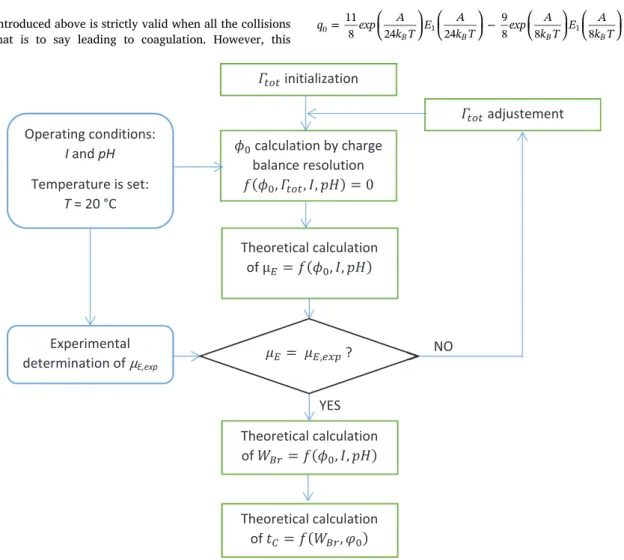
⎜ ⎟ = + ⎛ ⎝ ⎞ ⎠ ⎛ ⎝ ⎞ ⎠ = ∞ W q m Gκa K Aκam k T 1 1 2 1 ! 12 3 Br m m B 0 1 0 (17) ⎜ ⎟ ⎜ ⎟ ⎜ ⎟ ⎜ ⎟ = ⎛ ⎝ ⎞ ⎠ ⎛ ⎝ ⎞ ⎠ − ⎛ ⎝ ⎞ ⎠ ⎛ ⎝ ⎞ ⎠ q exp A k T E A k T exp A k T E A k T 11 8 24 24 9 8 8 8 B B B B 0 1 1 (18)

Fig. 1. Flowsheet describing the method to determine tc.

Using a simple charge balance, the following relation is then ob-tained:

= G π γ ε ε k T e κ 384 ( )2 2 r B 0 0 (19) where E1 is the 1st order exponential integral and K0the 0th order

modified Bessel function of the second kind.

As a consequence, it is possible to express a new Brownian kinetic kernel taking into account the inter-particulate forces for suspensions that are not fully destabilized through the use of WBr:

= k W k 1 Br Br Br ' (20) Eq. 14 is analogous to second-order chemical reaction kinetics and can be used to estimate a Brownian characteristic coagulation time (here assimilated to a half-life time) expressed as follows:

= = t k N W πμa k Tφ 1 c Br Br B ' 0 3 0 (21)

where N0is the initial number concentration of particles andφ0 the

volume fraction of the suspension (φ₀=N04πa₃

3

). Due to the simplifi-cations used to establish such a model, Eq. 20 should be considered qualitatively and not quantitatively; however, it can be of a great use to estimate whether a latex can be considered stable through time or not.

3. Materials and methods 3.1. Strategy

The strategy developed in this work to access the characteristic time of Brownian coagulation from pH and ionic strength values is sum-marised inFig. 1. The surface potentialϕ₀is estimated by solving the charge balance equation (Eqs. 11–13) using MATLAB with the FSOLVE function where the surface potential is taken as the variable. The the-oretical and experimental determinations of the electrophoretic mobi-lity are described in the next sections.

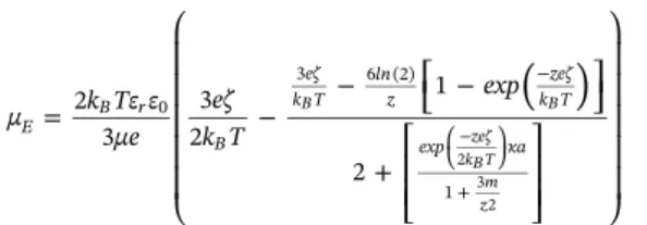
3.2. From surface potentialϕ₀to theoretical electrophoretic mobility μ_E The theoretical electrophoretic mobility can be calculated from the value of ϕ .₀ More precisely, the zeta potential is calculated for a given surface potential with Eq. 22, giving access to the corresponding elec-trophoretic mobility in Eq. 23.

⎜ ⎟ = ⎡ ⎣ ⎢ − ⎛_⎝ ⎞_⎠ ⎤ ⎦ ⎥ ζ k T

ze arctanh exp κx tanh zeϕ k T 4 . ( ) 4 B z B 0 (22) where xzrepresents the distance between the shear plane and the

sur-face of the particle. Eq. 22 is strictly valid for plane sursur-faces, however Behrens et al.[39]considered the precision of this equation satisfactory whenϕ0is estimated using Eq. 12, which takes the surface curvature

into account. For this study, xzis taken equal to 0.2 nm, which is a

physical order of magnitude for this distance[24].

= ⎛ ⎝ ⎜ ⎜ ⎜ ⎜ ⎜ − − ⎡ ⎣ − ⎤⎦ +⎡ ⎣ ⎢ ⎢ ⎤ ⎦ ⎥ ⎥ ⎞ ⎠ ⎟ ⎟ ⎟ ⎟ ⎟ − ⎛ ⎝ ⎞ ⎠ + −

( )

μ k Tε ε μe eζ k T exp 2 3 3 2 1 2 E B r B eζ k T ln z zeζ k T exp κa 0 3 6 (2) 1 B B zeζ kB T m z 2 3 2 (23) m is the drag coefficient equal to 0.184 [43]. Eq. 23 is proposed by O’Brien and Hunter for κ a ≥ 30 and |ζ| ≤ 250 mV. The modeling proposed in this study relies on equations strictly valid for symmetrical electrolytes. Even if a 1:2 electrolyte is added in the experiments in-troduced in this work, it has to be mentioned that in most of the ex-perimental cases presented here, the ionic strength is mainly due to the symmetrical background electrolyte, explaining this choice. Other modeling approaches can however be found in the literature. Ohshima et al.[44]proposed an approximate expression of electrophoretic mo-bility in the case of symmetrical electrolytes successfully applied[42]

and valid for κ a ≥ 10, that however comes with a more complex analytical expression. Also, in the case of mixed solutions (1:1 and 2:1 or 1:1 and 3:1 electrolytes), Nishiya et al.[45]proposed a modeling strategy from the surface potential to the electrophoretic mobility based on Ohshima approximations. As the electrolytes used in this study are 1:1 and 1:2, this approach was not considered here.

Table 1summarises the parameters considered in this study. The surfactant used to stabilize the latex is a carboxylic acid with a dis-sociation constant Kaequal to 10−5.

3.3. Electrophoretic mobility measurements 3.3.1. Set-up and coagulant

In order to measure the impact of both pH and I on the electro-phoretic mobility measurements, acid titrations are performed on latex with different initial ionic strengths. Measurements are performed using a Malvern Nanosizer ZS® and a MPT-2 titrator is used to ensure reliable pH adjustment. pH is monitored using a Malvern pH-probe (SEN0106). Each measurement is performed in a Malvern DTS1060 folded capillary cell. Industrially, pH-sensitive latex is often destabilized using sulfuric acid. For this reason, titrations are performed using H2SO4 at a

con-centration equal to 0.05 M. Measurements are performed from pH = 7.5 to pH = 1.5.

3.3.2. Latex

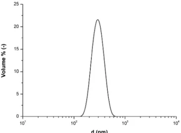
The latex used in this study is a core-shell PMMA/PABu copolymer, stabilized by a carboxylic acid surfactant. All the experiments are car-ried out using a suspension at initial concentration 1.375 × 10–3% (w/ w), obtained after initially diluting an industrial latex (33% w/w) using ultrapure water (Purelab® Option-Q). The volume-average radius of the latex particles is a = 141 nm (d = 282 nm), measured using a Malvern Nanosizer ZS®. The measured monomodal distribution is presented in

Fig. 2.

Four samples of 12 mL are used for the study. With the use of KCl as a background electrolyte, the initial ionic strength of the suspension is adjusted at four different values: 0 mM, 10 mM, 50 mM and 100 mM. 3.4. Ionic strength variation through the titration

While adding H2SO4to the latex, both the dilution and the addition

of an electrolyte will change the ionic strength of the suspension. For a volume of acid added Vadd, the ionic strength, I, can be expressed as

follows:

= +

+

I I I V

V V

acid init init

init add (24)

H2SO4is a dibasic acid (pKa,1=−3, pKa,2= 1.9). Since the pH

ranges from 1.5 to 7.5, only the weakest acidity is taken into account in order to propose an expression of Vaddand Iacidas a function of the pH.

Parameter type Symbol Value

Fixed xz 0.2 nm Ka 10–5 T 20 °C Adjusted Γ0 — Calculated φ0 Eq. 13 ζ Eq. 22 μE Eq. 23 Table 1

Using a straightforward balance, it is possible to write the following relations to calculate Iacidand Vacid:

= ⎛ ⎝ ⎜ ⎜ + + + + ⎞ ⎠ ⎟ ⎟ − − − − − − − I 1 2 10 4 10 2 10 1 2 acid pH pH pH 10 10 10 10 pH pKa acid pKa acid pH ( ) ( ) (25) = − − − + − − + V V H SO 10 2[ ] 10 add init pH H SO pH 2 4 [ ] 1 10pKa acid pH 2 4 ( ) (26)

A comparison between the calculated Vaddand experimental Vacid

(given by the NanoZS software) for the titration at Iinit= 10 mM is

presented inTable 2. The results show good agreement and allow to better calculate I, and thusκ.

4. Results

4.1. Determination ofΓtot

The model introduced earlier isfirstly used in order to adjustΓtot,

using the titration performed at Iinitequal to 100 mM. Good agreement

between experimental and theoretical results is obtained for Γtot= 0.15 nm−2, with a maximal relative difference between the

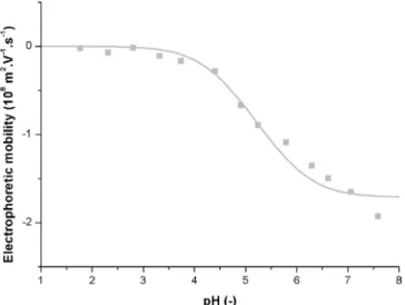
the-oretical and experimental electrophoretic mobilities of less than 1%. The comparison between the theoretical and experimental results can be seen inFig. 3.

The adjusted model (Model 1) is then used to predict the evolution of the theoretical electrophoretic mobility with pH for the four ionic strengths studied experimentally (Iinit= 0, 10, 50, 100 mM). The results

are presented inFig. 4.

At the highest ionic strengths studied (50 and 100 mM), the model and the experimental results are in good agreement over the whole pH range. For Iinit= 0 mM and 10 mM, however, the model clearly fails at

representing the electrophoretic mobility, particularly at low pH values (pH < 4). The model supposes that all the charges are brought by the carboxylic surfactant. Below pH = 3, almost all the surfactant mole-cules are thus in their acid form, i.e. without charges, and in this case the electrophoretic mobility should be null. However, especially at low ionic strength, the mobility is far from being null, which means that other species are very likely to be present on the surface of the particles. As a consequence, the theoretical model needs to be corrected to take into account this experimental fact.

4.2. Modification of the charge balance solved

To prepare the latex, the polymerization is triggered using sodium

formaldehyde sulfoxylate. In an aqueous medium, hydro-xymethanesulfinate ions will thus be present and in large majority compared with the other ionic species composing the latex. These ions are known to be unstable and to generate sulfoxylate ions in acidic mediums. As the ionic strength is increasing, these adsorbed ions will desorb further from the surface, in analogy with the desorption of ionic species in soils while increasing the ionic strength[46]. Several studies

[42,45,47]compute the adsorbed charge density using a Stern layer model. However, this approach needs data (notably the ion bulk con-centration) that is not given by the industrial latex provider. For this reason, a more straightforward model is used in this study.

The experimental results presented in Fig. 4 show that for Iinit= 100 mM the results seem to be independent of the presence of an

additional surface charge since the experimental and the theoretical results are in good agreement. However, they are slightly dependent for Iinit= 50 mM since the model slightly underestimates the

electro-phoretic mobility for pH values lower than 2.5.σ1' denotes this

addi-tional surface charge. Since no further data is provided on the possible desorption mechanism, the following expression, which assumes linear desorption with increasing ionic strength, is taken:

= − − σ e I I I Γion lim lim 1' (27) Ilimstands for the ionic strength value beyond which the desorption is

totally achieved and is chosen equal to 70 mM (order of magnitude for which the second surface charge seems to be absent). Eq. 27 is con-sidered for I < Ilim. If this is not the case,σ1'is set to 0. The following

balance is thus solved:

+ + =

σ1 σ1' σ2 0 (28)

By adjustingΓion to 0.03 nm−2, the results given inFig. 5are

ob-tained. At the lowest pH, it can clearly be observed that the behavior observed with this model (Model 2) is in better agreement with the experimental results. However, for Iinit= 0 mM, a significant difference

between the model and the experiments for pH values ranging from 2.5 to 5 is observed. This discrepancy can be interpreted as a limitation of the O’Brien and Hunter approximation at these pH values. Indeed, as mentioned before, Eq. 23 is proposed forκ a ≥ 30 and |ζ| ≤ 250 mV. These conditions are fulfilled in the present study except for Iinit= 0 mM and pH > 2.4.

For Iinit= 10 mM, the model deviates from the experimental data

considerably for pH > 5 due to the increase in mobility granted by the ion adsorption at low ionic strength. As the sulfoxylate ions appear in the acidic medium, at the highest pH, the effect of its adsorption at the particle surface on the charge balance should not be taken into account. This discrepancy therefore confirms that the extra surface charge is due to the presence of sulfoxylate ions.

The agreement of the model with ion adsorption (Model 2) with the experimental data was checked calculating the root-mean-square de-viation (RMSD, Eq. 29) given inTable 3.

∑

= − = RMSD N μ μ 1 ( )2 i N E E exp 1 , (29) It can be seen that except in the case Iinit= 10 mM, the deviation is

lower using Model 2, confirming an improved agreement of the model as observed visually.

Fig. 2. Particle size distribution of the initial latex obtained with Nanosizer ZS®.

Table 2

Comparison of experimental and calculated Vadd.

pH (–) Experimental Vadd(mL) Calculated Vadd(mL)

1.66 4.67 5.34

1.76 3.38 3.69

2.27 0.776 0.786

Despite these limitations, the model reproduces the experimental electrophoretic mobility trends fairly well and is therefore used to es-timate the surface potential as a function of pH and I. Indeed, for the purpose of developing a coagulation process (including the determi-nation of optimal residence times, stirring characteristics etc.), the conditions where the model of electrophoretic mobility does not fit with the experimental data (Iinit= 0 mM, pH > 2.4; Iinit= 10 mM,

pH > 5) should not be considered. It will be seen in the next section that characteristic coagulation times that are higher than 1000 s are estimated under these conditions, signifying that the suspension is only slightly destabilized.

4.3. Estimation of WBrusing the surface potential model

The optimized surface potential model obtained can be used in the analytical WBrexpression proposed by Ohshima. The value chosen for

the Hamaker constant, A, is 10−20J, which is a common order of magnitude for polymers (Ottewill[33]proposes A = 1.05*10−20J for PMMA, and A = 0.95*10−20J for PS).Fig. 6represents the evolution of log(WBr) as a function of pH for different initial ionic strengths (0, 10,

50 and 100 mM). The model considers that pH is adjusted using sulfuric acid and takes into account the variation in ionic strength introduced by the addition of the acid and its dissociation. As mentioned before, when WBrequals 1 (log WBr= 0), the colloidal suspension is fully

destabi-lized. As expected,Fig. 6shows that the stability of the studied latex decreases with the pH. Moreover, it is observed that the maximum pH required to obtain full destabilization increases with the initial ionic strength of the solution. This is due to the fact that the presence of positive charges in the salt weakens the surface potential of the parti-cles, thereby reducing the repulsive potential energy. Therefore, de-stabilization is obtained with a lower amount of acid in the presence of salt.

While these calculated stability ratios can be used for further kinetic modeling, it is also possible to extract very practical information for the

Fig. 3. Comparison between experimental (dots) and calculated (line) electro-phoretic mobilities for Iinit= 100 mM.

Fig. 4. Comparison between experimental (dots) and calculated (line) electro-phoretic mobilities for Iinit= 0, 10, 50 and 100 mM.

Fig. 5. Comparison between the experimental electrophoretic mobility (dots) and the adjusted calculated electrophoretic mobility (line) for Iinit= 0, 10, 50

and 100 mM.

Table 3

RMSD calculations.

RMSD(Model 1) (m2_.V−1_.s−1_{) RMSD(Model 2) (m}2_.V−1_.s−1₎

Iinit= 0 mM 7.76E−09 5.96E−09

Iinit= 10 mM 7.83E−09 7.53E−09

Iinit= 50 mM 1.77E−09 2.02E−09

Iinit= 100 mM 1.05E−09 1.05E−09

As for example, a suspension of the studied latex at pH = 3 and Iinit= 10 mM will have a t φc 0 value equal to 0.1 s. If we consider a

volume fraction of 0.01, the Brownian coagulation time of the latex will

be equal to 10 s. In this case, it is very likely that performing coagu-lation in a stirred tank may lead to poor PSD control as it corresponds to the order of magnitude of mixing time in very efficient stirred tanks. On the other hand, if the volume fraction of the suspension is 0.0002, the Brownian coagulation time equals 500 s, which is greater than con-ventional mixing times expected in stirred tanks. It is thus reasonable to perform coagulation in this type of device under these conditions.

5. Conclusion

Using theoretical considerations related to the Brownian kinetics of coagulation and the short-range interactions between particles, this paper presents an original methodology based on electrophoretic mo-bility measurements to ultimately estimate a characteristic coagulation time as a function of the ionic strength and the pH of the medium considered. The methodology is applicable to colloidal suspensions with very small initial particles (with diameters less than a few hundred nanometers) where coagulation is initiated by Brownian motion. The methodology is illustrated with an industrial latex that has a pH-sen-sitive stability. Whilst difficulties were encountered in modeling the electrophoretic mobility due to the probable presence of adsorbed ions at the surface of the particles, the electrophoretic model proposed re-produces the experimental trends relatively well, thereby suggesting that both the modeling approach and the estimation of the surface potential are sound. The charge model was then used to calculate the total interaction potential and ultimately the Brownian stability ratio and the Brownian coagulation time as a function of the pH and the initial ionic strength of the medium. This was performed assuming DLVO theory.

The overall methodology presented provides a tool for scientists providing a simple means to estimate the time required to obtain an observable coagulated state of a colloidal suspension as a function of the physicochemical conditions of the medium and the volume fraction of the particles. For engineers, knowledge of characteristic times is necessary to adequately choose the experimental conditions and the equipment to obtain an effective coagulation process. For industrial coagulation, it is necessary to perform the process without mixing limitations (between the coagulant and the colloidal suspension) in order to obtain aggregates of desired and constant quality. For the purpose of data acquisition, it is also important that mixing time is shorter than the characteristic coagulation time in order to avoid fouling of the reactor and to obtain a reliable estimation of coagulation kernels, as well as reproducible experiments.

Acknowledgement

This work was supported by the French National Research Agency (ANR) in the framework of the Scale-Up project (ANR-12-RMNP-0016).

Fig. 7. pH vs. Iinitto fully destabilize the latex.

experimenter. As we can see in Fig. 6, it is possible to obtain for a specific initial ionic strength the pH at which the suspension is fully destabilized. By representing this data on a master curve as presented in

Fig. 7, it is possible for the experimenter to identify the minimum pH-value to be reached to ensure full destabilization at a given pH-value of Iinit.

This information can be of great use if the objective is not to obtain specific WBr values but simply to ensure full latex destabilization.

4.4. Coagulation characteristic time vs. mixing time

Using Eq. 21, it is possible to convert the values of WBr into

Brownian coagulation times. The results are presented in Fig. 8. As Eq. 21 depends on the volume fraction of the suspension φ₀, the coagulation

times are presented under the form tcφ0, which allows the calculation of

the coagulation time over a wide range of φ₀. Eq. 21 is obtained

as-suming the collisions between particles are binary, which is no longer the case at high volume fractions: Fig. 8 can therefore be reasonably used for φ₀ values that are lower than 0.01 [48]. At higher volume

fractions, as multiple collisions can occur simultaneously, tcis likely to

be lower than that predicted by the proposed model. Depending on the physicochemical properties of the medium and the volume fraction of the suspension considered, the evolution of the coagulation time versus I and pH represents an interesting tool for an experimenter who re-quires information about the stability of the considered suspension in a more practical way than the stability ratio calculation. It is also inter-esting to see that for this specific latex, even considering a very low initial ionic strength, the coagulation time is minimal for pH values ≤1.8, thus indicating that the suspension is fully destabilized regard-less of the background electrolyte concentration. This information can be very useful for studying coagulation when full destabilization is most of the time desired. The methodology developed in this paper is thus useful for a scientist who is wants to estimate the lifetime of a specific latex as a function of the physicochemical properties of the medium and the conditions ensuring full latex destabilization.

The knowledge of the characteristic time of the coagulation process can be of great help for engineers. Indeed, such a methodology can be used to wisely choose the experimental conditions (pH, ionic strength and volume fraction) and the design of the coagulator so that the characteristic time of coagulation is greater than the mixing time, thus ensuring reproducible experiments and good quality products. Indeed, poor mixing of the colloidal suspension and the coagulant may cause zones with high concentration of coagulant, leading to very fast particle coagulation and thus degrading the global morphology of the final aggregates and product quality. Fig. 8 shows the orders of magnitude of mixing times in different mixing devices. For stirred tanks, mixing time ranges from few seconds (for the mixing in turbulent flow regime of non-viscous fluids using effective stirrer technologies and baffles) to several minutes (particularly when the viscosities of the fluids to mix are very different) [49–53]. Although stirred tanks are the most widely used technology to carry out coagulation processes at industrial scale, experiments of coagulation in Taylor-Couette reactors are very often carried out for data acquisition. Indeed, these reactors generally pro-vide homogeneous shear rate fields in the fluids (except close to the walls where edge effects appear) and so the modeling of the coagulation mechanism is simplified. Mixing times observed in Taylor flow devices range from 2 to 60 s [54]. Tubular reactors in the laminar flow regime,

which favors the formation of spherical aggregates, are also used

[55–60]. However, the laminar flow regime typically does not provide effective mixing and a mixing device should be used before the coa-gulator to mix the colloidal suspension and the coagulant. Intensified mixing technologies – predominantly continuous and miniaturized re-actors – have also emerged over the last decades and provide very short mixing time as represented in Fig. 8 [61,62].

References

[1] G.G. Odian, Principles of Polymerization, fourth ed., Wiley-Interscience, Hoboken, NJ, 2004.

[2] R.C. Elgebrandt, J.A. Romagnoli, D.F. Fletcher, V.G. Gomes, R.G. Gilbert, Analysis of shear-induced coagulation in an emulsion polymerisation reactor using compu-tationalfluid dynamics, Chem. Eng. Sci. 60 (2005) 2005–2015,https://doi.org/10. 1016/j.ces.2004.12.010.

[3] N. Furukawa, W. Okada, Analysis of the coagulation rate of MBS (methylmetacry-late-butadiene-styrene) polymer latex and strengh of coagula, Adv. Powder Technol. 5 (1994) 161–175.

[4] P.T.L. Koh, J.R.G. Andrews, P.H.T. Uhlherr, Flocculation in stired tanks, Chem. Eng. Sci. 39 (1984) 975–985.

[5] De Boer, Coagulation in turbulentflow: part I, Inst. Chem. Eng. 67 (1989) 301–307. [6] M. Soos, A.S. Moussa, L. Ehrl, J. Sefcik, H. Wu, M. Morbidelli, Effect of shear rate on aggregate size and morphology investigated under turbulent conditions in stirred tank, J. Colloid Interface Sci. 319 (2008) 577–589.

[7] T. Sugimoto, M. Kobayashi, Y. Adachi, The effect of double layer repulsion on the rate of turbulent and Brownian aggregation: experimental consideration, Colloids Surf. Physicochem. Eng. Asp. 443 (2014) 418–424,https://doi.org/10.1016/j. colsurfa.2013.12.002.

[8] C.-J. Chin, S. Yiacoumi, C. Tsouris, Shear-inducedflocculation of colloidal particles in stirred tanks, J. Colloid Interface Sci. 206 (1998) 532–545,https://doi.org/10. 1006/jcis.1998.5737.

[9] S. Melis, M. Verduyn, G. Storti, M. Morbidelli, J. Baldyga, Effect of fluid motion on the aggregation of small particles subject to interaction forces, AIChE J. 45 (1999) 1383–1393.

[10] D.L. Marchisio, J.T. Pikturna, R.O. Fox, R.D. Vigil, A.A. Barresi, Quadrature method of moments for population-balance equations, AIChE J. 49 (2003) 1266–1276. [11] L. Wang, R.D. Vigil, R.O. Fox, CFD simulation of shear-induced aggregation and

breakage in turbulent Taylor-Couetteflow, J. Colloid Interface Sci. 285 (2005) 167–178,https://doi.org/10.1016/j.jcis.2004.10.075.

[12] J. Pohn, Scale-Up of Latex Reactors and Coagulators: A Combined CFD-PBE Approach, Queen’s University, 2012.

[13] A. Falola, A. Borissova, X.Z. Wang, Extended method of moment for general po-pulation balance models including size dependent growth rate, aggregation and breakage kernels, Comput. Chem. Eng. 56 (2013) 1–11,https://doi.org/10.1016/j. compchemeng.2013.04.017.

[14] H. Zhao, C. Zheng, A population balance-Monte Carlo method for particle coagu-lation in spatially inhomogeneous systems, Comput. Fluids 71 (2013) 196–207,

https://doi.org/10.1016/j.compfluid.2012.09.025.

[15] R.I. Jeldres, F. Concha, P.G. Toledo, Population balance modelling of particle flocculation with attention to aggregate restructuring and permeability, Adv. Colloid Interface Sci. 224 (2015) 62–71,https://doi.org/10.1016/j.cis.2015.07. 009.

[16] M. Vlieghe, C. Coufort-Saudejaud, A. Liné, C. Frances, QMOM-based population balance model involving a fractal dimension for theflocculation of latex particles, Chem. Eng. Sci. 155 (2016) 65–82,https://doi.org/10.1016/j.ces.2016.07.044. [17] A. Passalacqua, F. Laurent, E. Madadi-Kandjani, J.C. Heylmun, R.O. Fox, An

open-source quadrature-based population balance solver for OpenFOAM, Chem. Eng. Sci. 176 (2018) 306–318,https://doi.org/10.1016/j.ces.2017.10.043.

[18] J.-M. Commenge, L. Falk, Methodological framework for choice of intensified equipment and development of innovative technologies, Chem. Eng. Process. Process Intensif. 84 (2014) 109–127,https://doi.org/10.1016/j.cep.2014.03.001. [19] J. Aubin, J.-M. Commenge, L. Falk, L. Prat, Process Intensification by

miniatur-ization, in: M. Poux, P. Cognet, C. Gourdon (Eds.), Green Process Eng. Concepts Ind. Appl. Science Publishers (CRC Press/Taylor & Francis Group), 2015, pp. 77–108. [20] F.E. Torres, W.B. Russel, W.R. Schowalter, Floc structure and growth kinetics for

rapid shear coagulation of polystyrene colloids, J. Colloid Interface Sci. 142 (1991) 554–574.

[21] L.G. Bremer, P. Walstra, T. van Vliet, Estimations of the aggregation time of various colloidal systems, Colloids Surf. Physicochem. Eng. Asp. 99 (1995) 121–127. [22] B. Derjarguin, L. Landau, Theory of the stability of strongly charged lyophobic sols

and of the adhesion of strongly charged particles in solution of electrolytes, Acta Physicochim. URSS 14 (1941) 633.

[23] E.J. Verwey, J.T. Overbeek, Theory of the Stability of Lyophobic Colloids, Elsevier, Eindhoven, 1948.

[24] B. Cabane, Chapitre 2 : La stabilité colloidale des latex, Latex Synth. Tec & Doc, Lavoisier, 2006.

[25] M. Fortuny, C. Graillat, T. McKenna, Coagulation of anionically stabilized polymer particles, Ind. Eng. Chem. Res. 43 (2004) 7210–7219.

[26] E.M. Lifshitz, The theory of molecular attractive forces between solids, Sov. Phys. JETP 2 (1956) 73–83.

[27] H.C. Hamaker, The London-Van der Waals attraction between spherical particles, Physica 4 (1937) 1058–1072.

[28] M. Elzbieciak-Wodka, M.N. Popescu, F.J.M. Ruiz-Cabello, G. Trefalt, P. Maroni, M. Borkovec, Measurements of dispersion forces between colloidal latex particles with the atomic force microscope and comparison with Lifshitz theory, J. Chem. Phys. 140 (2014) 104906, ,https://doi.org/10.1063/1.4867541.

[29] T.F. Tadros, Colloid Stability: The Role of Surface Forces, Wiley-VCH Verlag, Weinheim, 2007.

[30] H. Ohshima, Approximate analytic expression for the stability ratio of colloidal dispersions, Colloid Polym. Sci. 292 (2014) 2269–2274,https://doi.org/10.1007/ s00396-014-3257-1.

[31] J. Visser, On Hamaker constants: a comparison between Hamaker constants and Lifshitz - Van der Waals constants, Adv. Colloid Interface Sci. 3 (1972) 331–363. [32] J. Israelachvili, Intermolecular and Surface Forces, Academic Press, 1992. [33] R. Ottewill, Chapter 3 - stabilization of polymer colloid dispersions, Emuls. Polym.

Emuls. Polym. Wiley, Guildford, 1997, pp. 59–121.

[34] M. Gouy, Sur la constitution de la charge electrique a la surface d’un electrolyte, J. Phys. Theor. Appl. 9 (1910) 457–468.

[35] M. Gouy, Ann. Phys. (1917).

[36] D.L. Chapman, A contribution to the theory of electrocapillarity, Philos. Mag. Ser. 6 (25) (1913) 475–481.

[37] O. Stern, Zur theorie der elektrolyischen doppelschicht, Z. Elektrochem. Angew. Phys. Chem. 30 (1924) 508–516.

[38] A.L. Loeb, J.Th G. Overbeek, P.H. Wiersema, The Electrical Double Layer Around a Spherical Colloid, The M.I.T. Press, Cambridge, Massachussets, 1961.

[39] S.H. Behrens, D.I. Christl, R. Emmerzael, P. Schurtenberger, M. Borkovec, Charging and aggregation properties of carboxyl latex particles: experiments versus DLVO Theory, Langmuir 16 (2000) 2566–2575.

[40] M. Smoluchowski, Drei vortrage uber diffusion, Brownsche molekularbewegung und koagulation von kolloidteilchen, Phys. Z. Sowjetunion. 17 (1916) 557–599. [41] N. Fuchs, Uber die stabilitat und aufladung der aerosole, Z. Phys. 89 (1934)

736–743.

[42] M. Kobayashi, S. Yuki, Y. Adachi, Effect of anionic surfactants on the stability ratio and electrophoretic mobility of colloidal hematite particles, Colloids Surf. Physicochem. Eng. Asp. 510 (2016) 190–197,https://doi.org/10.1016/j.colsurfa. 2016.07.063.

[43] R.W. O’Brien, R.J. Hunter, The electrophoretic mobility of large colloidal particles, Can. J. Chem. 59 (1981) 1878–1887.

[44] H. Ohshima, T.W. Healy, L.R. White, Approximate analytic expressions for the electrophoretic mobility of spherical colloidal particles and the conductivity of their dilute suspensions, J. Chem. Soc. Faraday Trans. 2 (79) (1983) 1613,https://doi. org/10.1039/f29837901613.

[45] M. Nishiya, T. Sugimoto, M. Kobayashi, Electrophoretic mobility of carboxyl latex particles in the mixed solution of 1:1 and 2:1 electrolytes or 1:1 and 3:1 electrolytes: experiments and modeling, Colloids Surf. Physicochem. Eng. Asp. 504 (2016) 219–227,https://doi.org/10.1016/j.colsurfa.2016.05.045.

[46] R. Naidu, N.S. Bolan, R.S. Kookana, K.G. Tiller, Ionic-strength and pH effects on the sorption of cadmium and the surface charge of soils, Eur. J. Soil Sci. 45 (1994) 419–429.

[47] A. Hakim, M. Nishiya, M. Kobayashi, Charge reversal of sulfate latex induced by hydrophobic counterion: effects of surface charge density, Colloid Polym. Sci. 294 (2016) 1671–1678,https://doi.org/10.1007/s00396-016-3931-6.

[48] M. Lattuada, P. Sandkühler, H. Wu, J. Sefcik, M. Morbidelli, Aggregation kinetics of polymer colloids in reaction limited regime: experiments and simulations, Adv. Colloid Interface Sci. 103 (2003) 33–56.

[49] K.W. Norwood, A.B. Metzner, Flow patterns and mixing rates in agitated vessels, AIChE J. 6 (1960) 432–437.

[50] I. Bouwmans, The Blending of Liquids in Stirred Vessels, Delft Univ. Press, Delft, 1992.

[51] M. Kraume, Mixing times in stirred suspensions, Chem. Eng. Technol. 15 (1992) 313–318.

[52] W.-M. Lu, H.-Z. Wu, M.-Y. Ju, Effects of baffle design on the liquid mixing in an aerated stirred tank with standard Rushton turbine impellers, Chem. Eng. Sci. 52 (1997) 3843–3851.

[53] I. Houcine, E. Plasari, R. David, Effects of the stirred tank’s design on power con-sumption and mixing time in liquid phase, Chem. Eng. Technol. Ind. Chem.-Plant Equip.-Process Eng.-Biotechnol. 23 (2000) 605–613.

[54] A. Racina, Z. Liu, M. Kind, Mixing in Taylor-Couette Flow, in: H. Bockhorn, D. Mewes, W. Peukert, H.-J. Warnecke (Eds.), Micro Macro Mix. Anal. Simul. Numer. Calc. Springer Berlin Heidelberg, Berlin, Heidelberg, 2010, pp. 125–139, ,

https://doi.org/10.1007/978-3-642-04549-3_8. Fig. 8. Evolution oftc 0φ with pH for different Iinitvalues. Comparison with

[55] K. Higashitani, S. Miyafusa, T. Matsuda, Y. Matsuno, Axial change of total particle concentration in Poiseuilleflow, J. Colloid Interface Sci. 77 (1980) 21–28. [56] J. Gregory, Flocculation in laminar tubeflow, Chem. Eng. Sci. 36 (1981)

1789–1794.

[57] I.C. Tse, K. Swetland, M.L. Weber-Shirk, L.W. Lion, Fluid shear influences on the performance of hydraulicflocculation systems, Water Res. 45 (2011) 5412–5418,

https://doi.org/10.1016/j.watres.2011.07.040.

[58] G. Farid Vaezi, R.S. Sanders, J.H. Masliyah, Flocculation kinetics and aggregate structure of kaolinite mixtures in laminar tubeflow, J. Colloid Interface Sci. 355 (2011) 96–105,https://doi.org/10.1016/j.jcis.2010.11.068.

[59] K. Lachin, N. Le Sauze, N. Di Miceli Raimondi, J. Aubin, C. Gourdon, M. Cabassud,

Aggregation and breakup of acrylic latex particles inside millimetric scale reactors, Chem. Eng. Process. Process Intensif. 113 (2017) 65–73,https://doi.org/10.1016/j. cep.2016.09.021.

[60] K. Lachin, N. Le Sauze, N. Di Miceli Raimondi, J. Aubin, D.F. Fletcher, M. Cabassud, C. Gourdon, Towards the design of an intensified coagulator, Chem. Eng. Process. Process Intensif. 121 (2017) 1–14,https://doi.org/10.1016/j.cep.2017.08.003. [61] J.Z. Fang, D.J. Lee, Micromixing efficiency in static mixer, Chem. Eng. Sci. 56

(2001) 3797–3802.

[62] L. Falk, J.-M. Commenge, Performance comparison of micromixers, Chem. Eng. Sci. 65 (2010) 405–411,https://doi.org/10.1016/j.ces.2009.05.045.