Correlations between eddy heat fluxes and baroclinic instability

CORRELATIONS BETWEEN EDDY HEAT FLUXES

AND BAROCLINIC INSTABILITY

by

RICHARD ST. PIERRE

B.S., Lowell Technological Institute (1974)

SUBMITTED IN PARTIAL FULFILLMENT OF THE REQUIREMENTS FOR THE

DEGREE OF MASTER OF SCIENCE

at the

MASSACHUSETTS INSTITUTE OF TECHNOLOGY

January, 1979

Signature of Author ... ...

Department of Meteorology, January 19, 1979.

Certified by ... ...

Thesis Supervisor.

Accepted by ... ... Chairman, Departmental Committee.

2

-CORRELATIONS BETWEEN EDDY HEAT FLUXES

AND BAROCLINIC INSTABILITY by

RICHARD ST. PIERRE

Submitted to the Department of Meteorology on January 19, 1979 in Partial Fulfillment of the Requirements for

the Degree of Master of Science

ABSTRACT

The two-layer model baroclinic stability parameter, meridional surface temperature gradients, and monthly mean meridional stationary, transient and total eddy heat transports, computed as functions of latitude and long-itude for three individual Januaries, are described and discussed. Corre-lation analyses for all possible combinations are computed, and reCorre-lation- relation-ships between these quantities are discussed. The results indicate that no direct relationship exists between stationary eddy heat transports and baroclinically unstable conditions. However, a direct relationship is found between transient eddy heat tra--ports and baroclinically unstable conditions. For example, the correlation between the transient eddy flux and the two-layer instability parameter is .52, which is statistically sig-nificant at the 99% confidence level. However, the strength of the corre-lation suggests that the degree of baroclinic instability only accounts for some of the variation in the transient eddy heat transport. Apparently, other factors also play an important role in the forcing of transient eddy heat transports.

THESIS SUPERVISOR: Peter H. Stone

- 3

-ACKNOWLEDGEMENTS

I would like to express my gratitude to Professor Peter H. Stone, who supervised the research and writing of this thesis. Appreciation is also expressed to Judson E. Stailey, who initially suggested this topic and helped with the computer programming and initial work. Thanks is also due to Frank Marks for his help in computer programming.

I also want to thank the Air Force Institute of Technology for

providing me the opportunity to perform this research.

Finally, my sincere appreciation is expressed to my wife and son, whose unending patience, support, and love made this all possible.

4 -TABLE OF CONTENTS TITLE ABSTRACT ACKNOWLEDGEMENTS TABLE OF CONTENTS LIST OF TABLES LIST OF FIGURES

CHAPTER ONE. INTRODUCTION

1.1 Background

1.2 Brief Review of Previous Work

CHAPTER TWO. SOURCES AND DESCRIPTION OF DATA

-2.1 Meridional Eddy Heat Transport Data

2.1.1 Meridional Stationary Eddy Heat Transport Data 2.1.2 Meridional Transient Eddy Heat Transport Data

2.1.3 Total Meridional Eddy Heat Transport Data

2.2 Meridional Surface Temperature Gradient 2.2.1 Acquisition of Data

2.2.2 Data Characteristics

2.3 Two-Layer Model Stability Parameter

2.3.1 Model Stability Parameter Characteristics 2.3.2 Data Characteristics

CHAPTER THREE. METHODS OF ANALYSIS

3.1 Correlation Analysis

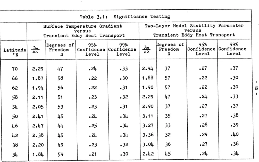
3.2 Significance Testing

CHAPTER FOUR. DISCUSSION OF CORRELATIONS

4.1 Meridional Surface Temperature Gradient versus

Two-Layer Model Stability Parameter

4.2 Meridional Stationary Eddy Heat Transport versus Meridional Transient Eddy Heat Transport

- 5

-4.3 Meridional Surface Temperature Gradient versus Meridional Stationary Eddy Heat Transport 4.4 Two-Layer Model Stability Parameter versus

Meridional Stationary Eddy Heat Transport 4.5 Meridional Surface Temperature Gradient versus

Meridional Transient Eddy Heat Transport 4.6 Two-Layer Model Stability Parameter versus

Meridional Transient Eddy Heat Transport

4.7 Meridional Surface Temperature Gradient versus Total Meridional Eddy Heat Transport

4.8 Two-Layer Model Stability Parameter versus Total Meridional Eddy Heat Transport

CHAPTER FIVE. SUMMARY AND CONCLUSIONS

5.1 Assessment of Results

5.2 Determining the Two-Layer Model Stability Parameter

and Meridional Transient Eddy Heat Transport Relationship

5:2.1 Investigating a Linear Relationship

5.2.2 Investigating a Power Relationship

5.3 Areas for Further Investigation REFERENCES

6

-LIST OF TABLES

Table Page

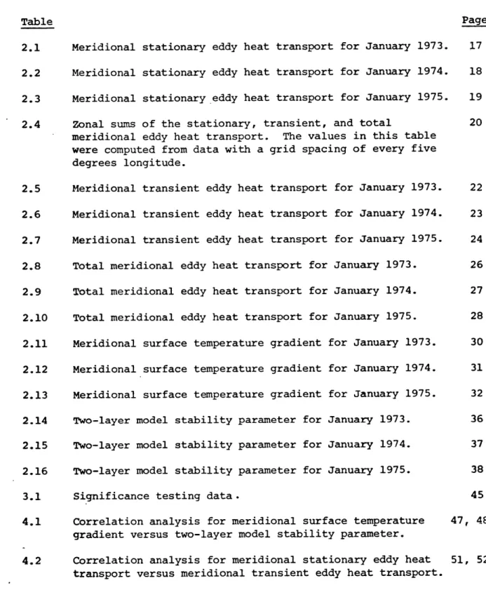
2.1 Meridional stationary eddy heat transport for January 1973. 17 2.2 Meridional stationary eddy heat transport for January 1974. 18

2.3 Meridional stationary eddy heat transport for January 1975. 19

2.4 Zonal sums of the stationary, transient, and total 20 meridional eddy heat transport. The values in this table

were computed from data with a grid spacing of every five degrees longitude.

2.5 Meridional transient eddy heat transport for January 1973. 22

2.6 Meridional transient eddy heat transport for January 1974. 23 2.7 Meridional transient eddy heat transport for January 1975. 24 2.8 Total meridional eddy heat transport for January 1973. 26

2.9 Total meridional eddy heat transport for January 1974. 27

2.10 Total meridional eddy heat transport for January 1975. 28

2.11 Meridional surface temperature gradient for January 1973. 30

2.12 Meridional surface temperature gradient for January 1974. 31

2.13 Meridional surface temperature gradient for January 1975. 32

2.14 Two-layer model stability parameter for January 1973. 36

2.15 Two-layer model stability parameter for January 1974. 37 2.16 Two-layer model stability parameter for January 1975. 38

3.1 Significance testing data. 45

4.1 Correlation analysis for meridional surface temperature 47, 48 gradient versus two-layer model stability parameter.

4.2 Correlation analysis for meridional stationary eddy heat 51, 52

-7-Page

4.3 Correlation analysis for meridional surface temperature 54, 55 gradient versus meridional stationary eddy heat transport.

4.4 Correlation analysis for two-layer model stability 56, 57 parameter versus meridional stationary eddy heat transport.

4.5 Correlation analysis for meridional surface temperature 59, 60 gradient versus meridional transient eddy heat transport.

4.6 Correlation analysis for two-layer model stability 63, 64 parameter versus meridional transient eddy heat transport.

4.7 Correlation analysis for meridional surface temperature 66, 67 gradient versus total meridional eddy heat transport.

4.8 Correlation analysis for two-layer model stability 69, 70 parameter versus total meridional eddy heat transport.

- 8

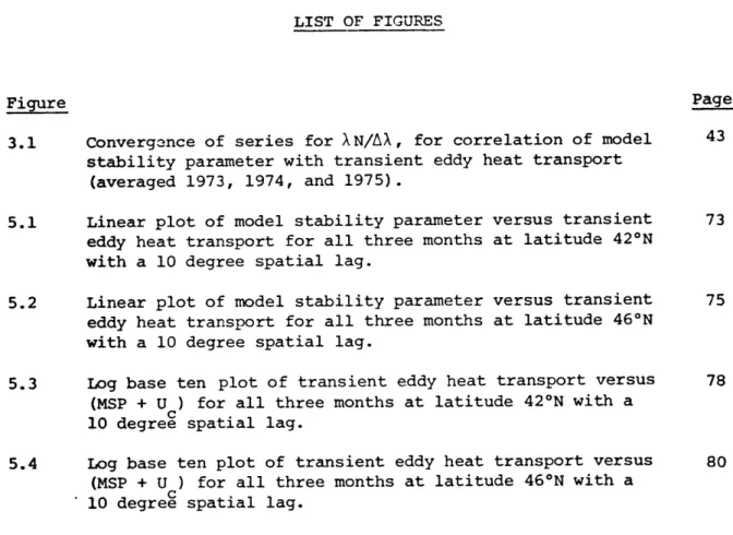
-LIST OF FIGURES

Figure Page

3.1 Convergence of series for XN/AX, for correlation of model 43 stability parameter with transient eddy heat transport

(averaged 1973, 1974, and 1975).

5.1 Linear plot of model stability parameter versus transient 73 eddy heat transport for all three months at latitude 42*N

with a 10 degree spatial lag.

5.2 Linear plot of model stability parameter versus transient 75

eddy heat transport for all three months at latitude 46*N with a 10 degree spatial lag.

5.3 Log base ten plot of transient eddy heat transport versus 78 (MSP + U ) for all three months at latitude 42*N with a

C

10 degree spatial lag.

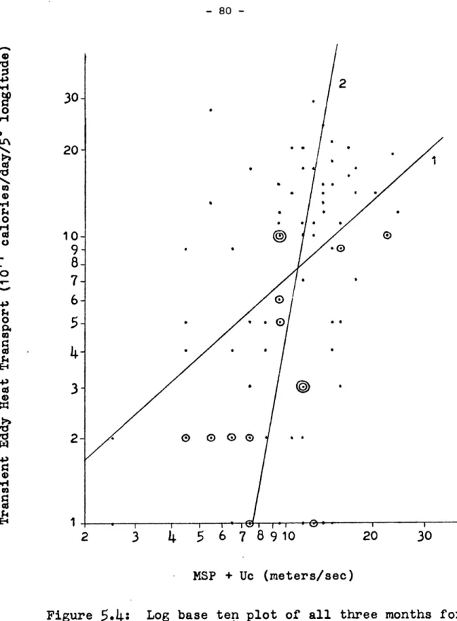
5.4 Log base ten plot of transient eddy heat transport versus 80

(MSP + U ) for all three months at latitude 46*N with a c

- 9

-CHAPTER ONE INTRODUCTION

1.1 Background

In the troposphere, the equator is warmer than the poles, and this is a result of radiational imbalances. We observe a net heating due to radiation at the equator, and at the poles a net radiational cooling occurs. If this was the only process working, the equator to pole temperature gra-dient would change and become larger. Looking at a long-term average, the

temperature structure of the atmosphere is essentially in equilibrium. For this condition to exist, heat must be transported poleward.

In the atmosphere, the south-to-north transport of sensible heat at a given time and location can be expressed mathematically as

HT = (pC AZ)VT (1.1)

p

where HT is the local south-to-north sensible heat transport, V is the south-to-north wind component, T is the absolute temperature, C is the

p

specific heat of dry air at constant pressure, p is the density of the air, and AZ is the thickness of the layer in which the heat transport is to be computed. In developing the thermodynamic equation for practical use and study, this transport is often averaged over an appropriate time interval and averaged zonally (i.e. averaged around a latitude circle). This averaging may be represented symbolically by:

[HT] = (pC AZ)[VT] (1.2)

- 10

-where the bar represents a time average and the brackets represent an average around a latitude circle. Equation 1.2 represents the mean meri-dional heat transport. This transport is commonly broken down into three components by expressing the individual instantaneous values, V and T, in terms of their means and anomalies, as

V = V + VI, V = [V] + V*, T = T + T', T = [T] + T*

The bars and brackets have their previously defined meanings, and the prime and asterisk superscripts represent departures from the time and

space averages, respectively. By making the above substitutions, we see that

[VT] = [V][T] + [V*T*] + [V'T'] (1.3)

recognizing that the time and zonal averages of the departures are zero

by definition.

The first term on the right hand side of equation 1.3 represents the heat transport due to the mean meridional circulation. This is the heat transport due to the Hadley, Ferrel, and Polar cells. The last two terms represent the meridional eddy heat transport broken down into its components. The term [V*T*] depicts the standing or stationary eddy heat transport. Stationary eddies are waves in the mean flow that persist over the averaging time period. For example, if we select an averaging time of a month, then the waves on a monthly mean 500 mb map would be stationary eddies. The last term in equation 1.3 represents the meridional transient eddy heat transports. Transient eddies are all deviations in tht- eddy

---- 11

-circulations within the averaging time period. For example, according to Clapp (1970), if the averaging time interval is a month, transient eddies are the part of the mean meridional heat transport due largely to travel-ing cyclones and anticyclones.

Steady state models used to simulate climate cannot calculate transient eddy heat transports. The other two terms (the stationary eddy and mean meridional circulation heat transports) involve the covariance or product of the time-averaged quantities and can, therefore, (at least in principle) be predicted explicitly by a steady state model (Clapp, 1970). For this reason, studies have been directed toward the understanding and parameterization of the transient eddy heat transports.

1.2 Brief Review of Previous Work

Parameterization of transient eddy heat transport using an "Aust-ausch coefficient" approach was originally proposed by Defant (1921). In this approach, the transient eddy heat transport term in equation 1.3 is approximated by

[T'V'] = -K(a[T]/3Y) (1.4)

where the bar and brackets signify time and zonal averages as before, and K is the Austausch coefficient. White and Jung (1951) were among the first to estimate the Austausch coefficient using mean heat transports

computed from synoptic weather maps. In their study, they also observed

a negative correlation between eddy heat transports and temperature

- 12

-not separate stationary and transient eddy components in their

computa-tions. Later Saltzman (1967), basing his ideas on the

linear-pertur-bation form of the hydrodynamic and thermodynamic equations, suggested that

K = -B(a[T]/3Y) (1.5)

where B is a stability coefficient. Substituting equation 1.5 into

equa-tion 1.4 gives

[T'V'] = B(a[T]/3Y)2 (1.6)

indicating that the transient eddy heat transport is proportional to the square of the temperature gradient.

. Clapp (1970) used two independent sets of data to obtain new esti-mates of K and B, and investigated the Austausch formulae. His investiga-tion suggests that the Austausch formulae may be fairly successful in es-timating the zonally averaged meridional transport. In attempting to ex-tend this test to explain longitudinal variations, his preliminary efforts were not successful. This suggests that further investigations and obser-vations of meridional eddy heat transports are needed, especially studies containing longitudinal variations.

Oort and Rasmusson (1971) have compiled a very complete set of computed transports for the five year period May 1958 to April 1963. Their

computations included meridional heat transports for each month broken down into the three components described previously. All their work was direct-ed at zonally averagdirect-ed quantities, so they could not observe longitudinal differences. Latitudinal, seasonal and monthly variations in the heat

-- 13

-transports were observed and discussed. Many of their observations are relevant to our investigation, and we will refer to their work often in

the course of this paper.

Blackmon et al. (1977) performed an observational and statistical study of heat fluxes. They used time-filters to study fluctuations of different periods. The most definitive results involved "band-pass"

fluc-tuations (flucfluc-tuations having a period of 2.5-6 days) which appeared to be associated with developing baroclinic waves. Their investigation suggested a relationship between poleward eddy heat fluxes and baroclinic instability associated with the strong thermal gradients at the earth's surface. This is one of the results that influenced the structure of our study.

The main motivation for our study was a paper by Stone (1978). In his paper, he compared zonal mean meridional temperature gradients in the atmosphere to critical temperature gradients predicted by a two-layer baro-clinic model. Stone observed that eddy heat fluxes are sensitive to changes in meridional temperature gradients (i.e. baroclinic instability). This observation suggests a relationship between these two quantities.

We intend to statistically investigate the relationship between meridional eddy heat transports, meridional surface temperature gradients, and the two-layer model stability parameter, since baroclinic theory and results from previous studies have suggested a possible relationship be-tween these quantities. We will deal only with the Northern Hemisphere, where the raw data are more abundant. In order to observe latitude and longitude variations, quantities were used which had been calculated for evenly spaced grid points. In this study, values of the total tropospheric

- 14

-meridional eddy heat transport were used which were defined as follows: h

EF= pc (V-[V]) (T-[T])dZ (1.7)

0

A time averaging period of a month was used, and h is the height of the

tropopause. This flux was divided into two components. The meridional stationary eddy heat transport at each grid point was computed from the equation

h

SE

J

pC

(V*T*)dZ

(1.8)

0

i.e., SE represents the monthly mean meridional stationary eddy heat trans-port. Once the stationary and total eddy heat transport were computed, a transient eddy heat transport was simply determined by subtraction,

TE = EF - SE (1.9)

where TE is the monthly mean meridional transient eddy heat transport. It is important to note that fluctuations in the meridional mean circulation are not included in the TE term, but are included in the transient eddy heat transport term in equation 1.3.

With the quantities calculated at each grid point, we are able to perform a correlation analysis for all possible combinations of these quan-tities. We will concentrate our investigation on longitudinal variations, since this area has not been explored. Once the correlation analysis is perfo:rmed, empirical parameterization schemes for the meridional transient eddy heat transport will be investigated.

- 15

-CHAPTER TWO

SOURCES AND DESCRIPTION OF DATA

2.1 Meridional Eddy Heat Transport Data

The meridional eddy heat transport data was calculated at the Goddard Institute for Space Studies (GISS), under the direction of

Pro-fessor Peter H. Stone, Massachusetts Institute of Technology. The raw data for the calculations was provided by the National Meteorological Cen-ter (NMC). Mean monthly values of eddy heat transport were available for

January 1973, 1974, and 1975. The data was recorded for every four degrees

of latitude 900S, 860S, ... 860N, 90*N, and every ten degrees of longitude

1750W, 1650W, ... 165*E, 1750E. This study was based on the data between 18*N and 70*N latitude. All the meridional eddy heat transport data are

vertically averaged values for the troposphere, and are in units of 1017 calories per day per five degrees longitude with positive indicating northward. Before the vertical averaging, the tropopause was determined separately for each grid point. The meridional eddy heat transport data was separated into stationary eddy and transient eddy components for the monthly mean data.

2.1.1 Meridional Stationary Eddy Heat Transport Data

Oort and Rasmusson (1971) observed that the meridional stationary eddy heat transports (MSEHT) were strongest in the winter. This is one of the main reasons the month of January was used for our study. Haines

- and Winston (1963) first noted that the MSEHTs were dominated by three main features, the Aleutian low, the Icelandic low, and the Siberian high

- 16

-pressure systems. They also observed that the peaks of the transports are

located to the east of these features, i.e. the transportof coldair

south-ward by the northerly flow over eastern Siberia and the transport of warm air northward over the central North Atlantic and Gulf of Alaska. The exact position and relative importance of these features varies from year to year, as pointed out by Blackmon et al. (1977). Tables 2.1, 2.2, and

2.3 contain the MSEHT data for our three months. From the tables, we can

see that the Icelandic low was very strong and the dominant feature for the monthly mean MSEHT in January 1973. For January 1974, all three fea-tures were strong, but the Icelandic low was still slightly dominant and

shifted 20*E of its previous years position. In January1975, the Siberian

high and the Aleutian low pressure systems were the dominant features.

. The latitude of the peak MSEHT fluctuates annually. Table 2.4

con-tains the MSEHT summed around each latitude circle. By examining the summed values of our MSEHT, we see the peak transport occurred at 58*N for January

1973. In January 1974, the peak MSEHT was located at 46*N. January 1975's

peak was situated at 50*N. These fluctuations from year to year indicate not only the variability of the transports, but also that we have avariety of data to study, rather than a bias sampling of one particular case. The position of the peak MSEHT for the average over the three months was at latitude 500N. Oort and Rasmusson (1971) also found the peak MSEHT in this

location with data over a five year period.

2.1.2 Meridional Transient Eddy Heat Transport Data

The meridional transient eddy heat transport (MTEHT) is of the same order of magnitude as the MSEHT, when comparing the summed values in Table

Stationary Eddy Hoat Flup Jonuary 1973 Long itude 17S 165 155 14S 135 125 115 105 95 'e5 75 85 S9 45 39 29 15 5 5 15 25 35 45 55 5 75 95 95 105 115 125 135 145 155 165 175 70 -2 -1 0 0 0 -1 -1 0 3 4 3 0 4 3 14J 27 29 25 I 15 0 -11 -15 -10 2 3 -2 -3 S 8 1 -5 10 15 6 -5

9

H

11

-3

11 22 14 -1 12 23 13 -1 13 18 4 -3 13 7 -5 -3 6 0 -7 -2 2 1 -3 -1 2 1 0 0 1 0 0 -1 1 0 00 -1 4 -2 3 -5 1 -7 -2 -8 -4 -7 -4 -3 -2 0 3 1 7 3 9 ? 11 5 7 -2 1 1 3 0 a 3 12 3 16 3 18 6 22 11 18 11 9 9 3 5 1 3 4 3 7 8 51 53 37 15 -5 -16;21I -11 37 66 37 8 -8 -18:-23 -9 46 7 63 4 -4 -10 -14 -18 -6 48 F6 47 8 -11 -10 -10 -10 -2 45 53 29 -7 -13 -S -6 -4 1 37 36 10 -17 -14 0 -2 -1 1 ?3 17 -2 -16 -10 0 0 0 1 6 2 -6 -7 -1 0 -1 0 0 1 -4 -3 0 7 0 -4 0 0 1 -2 0 4 9 2 -7 -2 1 3 -1 1 6 7 2 -8 -4 2 2 -3 0 5 4 1 -8 -5 1 0 6 4 0 4 10 4 -2 8 11 0 -7 9 8 -10 -14 11 1 -15 -13 9 -6 -9 -5 6 -9 -3 1 3 -6 -3 0 2 -1 -2 5 0 0 0 14 -1 -1 0 0 -3 -3 0 1 -3 -1 1 1 66 62 L 58 A 54 T 50 I 46 T 42 U 38 D 34 E 30 26 22 18 0 .1 1 2 2 2 5 1 4 2 3 3 1 3 -3 3 -4 3 -3 0 0 -2 4 -1 0 1 -1 2 -3 3 -4 5 -S 6 -2 9 4 12 3 11 0 8 -5 1 -1 -1 1 -3 1 -3 1 -3 1 -3 2 0 1 2 -1 -5 -4 70 5 6 8 6 9 15 20 11 13 21 25 16 16 24 20 17 14 24 18 13 11 21 16 5 11 16 a 0 7 9 4 1 4 5 4 8 4 8 10 14 4 9 a 11 3 4 2 6 1 2 50 -1 -6 -5 66 -2 -7 -S 62 -2 -7 -5 5 3 -5 -4 54 4 -3 -2 50 1 -1 2 46 0 3 5 42 6 9 7 3 12 11 3 34 11 7 -9 30 6 3 -15 26 6 -3 -12 22 -4 -11 -9 18 175 165 155 145 135 125 115 105 95 85 75 65 55 45 35 25 15 5 5 15 25 35 45 55 65 75 85 95 105 115 125 135 145 155 165 175

Table 2.1

3 1 1 3 1 1 0 -1 0 -1 -1 -3 -6 0 0 1 -1 2

Stationary Eddy Heat Flux January 1974 Longitude 1J7 165 15 145 135 125 115 185 96 86 75 65 5 45 35 25 15 5 5 15 25 35 45 55 6s 75 S5 95 105 115 125 135 145 155 165 175 0 -2 -4 -5 -2 6 14 16 9 -1 -2 -2 1 0 -3 -6 -6 3 16 12 -2 -2 2 5 6 -1 -7 -10 -4 11 19 15 1 0 6 14 20 6 -6 -11 -10 1 14 14 6 0 12 21 33 26 6 -16-13 -9 4 7 5 2 11 21 34 62 22-19 -14 -9 -3 2 1 1 S 18 32 59 35 -16 -16 -6 -5 2 7 3 --1 14 26 48 41 10 -16 -4 -1 11 20 7 -2 11 22 35 38 -5-16 -4 4 22 26 11 -2 9 18 22 24 1 -13 -1 8 0231 1814 -6 4 8 8 14 6 -8 0 8 13 11 10 1 -2 -5 3 11 3 1 -2 4 10 S S 0 -8 10 2 6 1 2 2 1 0 1 0 0 -10 -9 0 0 2 1 1 -2 -2 -1 -1 2 11 16 I 0 -8 -1 -3 2 0 4 1 0 1 0 37 36 19 8 1 -1 S, 47 20 8 -2 -5 E 51 19 6 -3 -4

6

43

8

0

-4 -1

0 -9 -6 -2 2 Al 12 -15 -9 1 4 24-10 -10 -3 3 3 3-2 2 -6 7 3 -2 -4 -18 1 18 1 -7 -2 -1 12 -1 -9 1 4 16 a -7 -10 2 1 12 18 -14 -10 1 8 5 6 -7 -8 0 0 0 0 -1 1 2 3 6 9 8 13 2 7 -4 0 -5 -1 -5 1 -3 0 -1 -2 -1 -1 -3 1 -4 -5 -5 -5 -5 -2 -1 -3 -5 -2 2 -3 -8 -7 -3 3 8 -8 -4 -2 1 7 1 5 2 -2 11 11 14 9 0 9 14 26 22 11 7 14 34 39 23 4 10 31 27 1 6 19 30 16 -1 4 12 13 6 0 10 12 4 S 4 12 13 3 2 1 7 7 5 0 -3 -3 8 2 1 175 166 155 145 135 15 115 105 95 OS 75 SS 5 45 36 25 15 5 5 15 26 3S 4 SS SS 7S 86 95 10115 12S 13S 145 15 165176

Table

2.2

L A T I T U D0 E 1 70 1 66 2 62 5 58 8 S4 9 50 6 46 3 42 8 38 12 34 6 30 0 26 -3 22 -6 18

175 165 155 145 135 125 115 105 95 S5 7S 85 95 45 70 0 0 0 0 1 3 3 6 7 66 0 0 0 1 0 0 1 5 12 62 0 0 0 3 2 -2 0 2 13 L 58 0 3 3 7 8 -1 -5 0 9 A 54 2 7 8 12 13 -2 -9 -2 6 T 50 3 14 18 22 12 -8 -13 -6 4 146 6 21 28(3) 7,-ii-15 -9 2 T 42 10 28 29 28 91-33:-16 -7 1 U 38 10 26 20 20 8.-32:-14 -3 3 0 34 1 15 11 12 2 -13 -8 0 6 E 30 -6 3 3 4 2 -5 0 0 -1 26 -8 -4 0 1 1 -1 0 -3 -4 22 -8 -6 -1 0 0 1 -2 -2 -6 18 -8 -5 -1 -1 -1 0 0 -1 -3 -4 -1 -3 -3 -1 -1 I 1 1 3 2 4 3 7 3 6 -1 -4 -6 -11 -7 -9 -3 -4 0 0 1 0

Stationary Eddy Heat Flux January 1975 Long itude 35 25 15 5 S 15 25 0 -1 -3 0 8 0 4 -1 2 3 11 17 9 3 2 8 18 24 18 6 -2 8 11 27 29 12 -3 -10 15 13 29 16 7 -14 -14 16 16 2 9 -1 -16 -11 12 14 5 0 -9 -9 -S 8 4 -3 -4 -10 -1 1 1 -3 -4 -1 -4 8 4 -1 -3 0 1 2 10 3 -1 1 2 1 2 3 3 1 0 Z I 1 -1 2 1 -1 e 1 0 -1 0 0 -1 -1 1 0 0 0 35 45 55 65 75 86 95 105 115 125 135 345 155 165 175 0 0 0 -1 0 0 1 0 0 4 1 3 S 4 10 2 9 16 11 12 4 15 29 22 L3 4 14 37 33 21 1 10 37 37 28 -2 6 25 20 -1 2 0 -1 2 8 6 2 0 2 4 6 3 2 4 5 3 3 2 3 7 -1 2 0 1 2 2 2 1 0 0 70 3 1 -1 0 66 4 -1 -1 -1 62 6 -2 -2 -1 59 8 -2 -5 -3 54 6 -S -8 -4 50 2 -12 -9 -3 46 -1 -11 -2 2 42 -2 2 7 4 38 9 13 9 -1 34 9 13 0 -10 30 7 7 -7 -13 26 4 1 -8 -11 22 0 0 -5 -6 18 175 165 ISS 145 135 125 115 105 95 85 75 65 55 45 35 25 15 S 5 15 25 35 45 55 65 75 85 95 105 115 125 135 145 155 165 175

Table

2.3

Latitude

MSEHT

MTEHT

Total EHT

*N

(10

19 cal/day)

(10

19 cal/day)

(1019 cal/day)

1973

1 .79

3.51

5.12

5061

5.29

4.85

3.75

2.48

1

.69

1

.63

1

.56

1.30

0*61

-. 43

1974

2.76

4.24

5.60

6.15

6.10

6.o27

6.35

5.26

4.07

3.35

2.86

1

.70

-.₀₂

-.38

1975

o.65

1

.31

2.23

3*00

3.60

3.80

3059 2099

2.14

1

.35

0.53

0002 - _.40

-. 50

1973

1

.66

2.10

2067

3.18

3.77

4.80

5081 6034

5.82

4.21

2.33

1

.11

0.41

I .1 _____ ____I

1974

1.47

1

.70

1.74

2.05

2*97 3080

3.63

2.89

2.27

1,.85

1.13

0.43

0.04

-. 10

1975

2.29

2.73

3.13

3.63

4.15

4.69

4.79

4.66

4.20

3.02

1.54

0.46

0.03

-- 11

1973

3.46

5.61

7079

8.79

9.06

9.64

9.56

8.82

7.51

5.83

3.89

2.41

1.02

-- 38

1974

4.23

5.93

7.34

8020

9007

10.07

9.98

8.15

6.34

5.21

3*99

2.14

0.03

-. ₄₈

1975

2.94

4-04

5.36

6.63

7.75

8.49

8.38

7.65

6.34

4.37

2.07

0.48

-. 37

-.61

Table

2.4

70

66

62

58

54

50

46

42

38

34

30

26

22

18

- 21

-2.4; however, the peaks of the MSEHT are generally larger than the peaks of the MTEHT. The MTEHT are spread more uniformly over the globe than the

MSEHT. Even though the MTEHTs are dispersed around the globe,

there are locations where peak transports do exist. Tables 2.5,

2.6, and 2.7 display the transient compound of the meridional

eddy heat transports. Notice that the position of the peaks supports the observation made by Blackmon et al. (1977) that the peaks are closely related to the major storm tracks. Three major storm tracks, along the east coast of the United States extending to Greenland, along the east coast of Asia up to Alaska, and a

short track along the west coast of the United States and Canada,

are primarily emphasized by our data. The exact position and strength of these peaks varies annually. In January 1973, the peaks were mainly along the east coasts of Asia and the United

States. These two peaks were again the dominant features in

January 1974; however, they were displaced further north and east

of the previous year's position. January 1975 was dominated by three peaks. The peaks along the east coasts of Asia and the United States were still evident and were located primarily be-tween the January 1973 and January 1974 positions. A third peak was located along the west coast of Canada and the United States.

It was smaller in area coverage but of the same magnitude as the other two peaks. The variability of these peaks reflect the variability of the storm tracks from year to year.

iranelnt Eddy Heat Flux Jonuary 1973 Long I tude 175 165 155 145 135 125 115 186 95 95 79 SS 9 49 35 25 15 5 S 15 25 35 45 55 65 75 85 96 185 115 125 135 145 155 165 175 8 16 15 9 1 0 1 3 4 3 2 3 4 3 4 2 1 1 1 2 2 1 -1 -2 -2 -2 0 -1 -2 -4 -2 -1 0 3 6 5 70 11 2 21 6 -3 0 2 6 6 4 2 4 4 4 9 0 -2 -1 1 0 1 4 -1 -4 -2 -1 1 0 -2 -2 0 1 1 4 6 4 66 11 22 2 -4 4 6 7 8 5 2 7 9 7 8 0 -S -1 1 -2 0 4 -5 -5 0 0 1 1 0 0 2 3 1 3 6 5 62 8 23 16 -4 -2 10 11 7 11 8 8 10 15 16 13 2 -9 -1 -1 -2 -3 1 -6 -4 0 1 1 2 4 3 3 4 0 1 6 6 50 9 12 12 -1 -2 14 13 6 12 13 12 12 22 26 18 6 -1 -2 -1 -2 -6 -1 -6 -3 1 1 1 0 3 5 3 3 0 2 4 6 54 8 10 13 4 0 14 11 2 10 17 18 13 24

(

18 7 6 -1 -4 -1 -3 0 -7 1 4 2 1 0 2 6 4 3 2 4 6 10 50 11 10 14 10 1 12 6 -1 10 20 26 17 24 29 17 10 9 -1 -6 1 2 2 -4 S 4 2 0 1 3 6 S 5 7 10 13 14 46 14 9 13 12 4 8 5 1 15 22 15 16 21 9 4 -1 -5 5 5 3 0 6 2 2 1 2 4 6 5 10 14 17 18 42 13 8 10 9 3 4 6 5 19 21 11 10 17 15 13 5 -1 -1 -3 7 8 1 3 4 3 1 0 1 5 5 4 14 16 15 19 19 38 12 11 7 4 -3 2 6 6 20 16 6 4 11 9 6 1 -2 1 -1 7 7 3 S 1 2 2 -8 -3 5 3 3 11 13 10 14 IS 34 6 9 3 1 -6 1 5 8 20 11 1 3 7 4 2 -1 -2 1 0 6 5 3 s -1 2 3 -8 -1 3 0 0 4 4 4 7 10 30 4 4 0 -1 -4 -1 3 4 12 6 0 2 5 2 0 -1 -1 0 0 4 3 4 2 1 3 2 -2 -2 0 0 -1 0 1 2 2 5 26 3 2 -1 -2 -3 0 1 2 4 3 1 1 3 1 -2 -1 0 2 -1 1 3 5 -2 -1 1 0 -1 -1 0 0 -1 -1 1 1 1 2 22 -1 0 -1 -1 -2 0 0 2 0 2 1 1 1 -1 -1 0 1 1 0 0 0 5 0 -1 0 -1 -1 1 0 1 -2 -1 0 0 2 0 18 175 165 155 145 135 125 115 105 85 75 65 55 45 35 25 15 5 r IS 25 35 45 55 65 75 85 95 105 115 125 13S 145 155 165 175

Table

2.5

70 66 62 L 58 A 54 T 50 1 46 T 42 U 38 D 34 E 30 26 22 19

iransient Eddy Heat riux January 1974 Longitude 175 165 155 145 135 12S 115 105 95 85 75 65 99 45 39 25 IS 5 5 1S 25 35 45 S5 65 75 8S 95 LOS 115 12S 13S 145 195 165 175 11 3 -2 -6 -3 a 0 -1 -1 -1 1 I 1 2 17 24 15 1 -6 -9 -3 3 3 0 -1 0 1 1 1 2 14 29 20 1 -9 -9 0 7 4 1 0 2 1 1 0 3 9 29 29 0: -16-6 8 10 4 1 3 6 3 0 2 9 5 21 3 -19 2 19 13 2 -3 9 12 8 5 12 12 1 1 33 9 -9 10 10 -1 -3 11 12 11 12 0 9 27 3 2 17 15 1 -1 0 10 12 10 14 7 2 13 19 9 10 1 7 - 0 1 -7 12 7 6 7 3 -7 14 10 2 15 12 0 -6 2 1 4 6 6 2 4 2 7 9 2 2 14 8 -6 -3 -1 3 2 S 2 2 3 1 S 6 -2 0 6 4 -7 -2 1 1 3 0 1 2 2 1 4 2 -2 -1 3 0 -4 -2 -1 0 2 0 0 2 0 1 2 1 -2 -1 0 -1 -1 -1 a 0 0 0 0 2 -1 -1 10 1 2 -3 -1 -2 -1 9 -1 S 0 0 S -2 5 -1 0 4 4 3 3 S 6 4 3 0 -1 -2 -2 2 1 1 1 3 S 6 S 4 0 -3 -2 -3 2 -1 -1 -3 2 6 0 3 S 1 -4 -1 -3 3 0 -3 -4 -1 3 -3 2 4 2 -2 --1 1 5 0 -1 -3 -4 0 -2 1 3 3 1 2 3 6 1 1 -4 -1 -1 1 2 3 2 3 2 4 S 3 0 -6 2 0 1 2 3 1 1 1 3 3 0 -1 -7 2 2 0 2 3 1 1 0 1 2 -1 -2 -5 4 1 0 2 5 1 1 0 1 1 -1 -4 -1 4 1 3 1 6 0 0 0 1 1 1 -2 1 S 2 4 0 3 0 -1 -1 2 2 2 -1 1 7 3 -1 -2 -1 -1 -1 -1 0 1 1 0 0 6 6 -6 -1 -2 -2 -1 -1 0 a 0 0 0 a 6 0 a a -2 -1 -1 1 0 2 4 0 -4 3 70 1 4 4 5 2 -3 2 66 0 S 3 2 3 1 2 62 0 4 -1 0 4 5 4 SS 2 0 -4 -3 1 6 6 64 4 -2 -3 -2 -2 4 6 50 4 0 0 1 -1 2 6 46 2 3 3 2 3 3 3 42 2 6 5 4 5 3 1 3 6 6 6 4 6 3 -1 34 3 4 3 4 2 0 0 30 2 3 2 1 1 0 1 26 1 0 1 a 0 1 0 22 1 -1 0 a 0 I 0 is 175 165 165 146 136 12S 116 105 95 95 76 65 6 45 36 26 1S S 5 16 26 35 46 55 6 75 85 36 105 116 126 135 14S 155 166 175 I

Table

2.6

70 66 62 L S8 A S4 T SO 1 46 T 42 U 38 D 34 E 30 26 22

4T

Tq

El

541 S91 SST SO'T SE1 521 S11 SOT S6 58 55 S9 SS 5* SC S2 ST S S ST 52 SE SIP SS SS S4 Se SG SOT SIT SZI SET SbiP SST 591 551 ST 0 0 0 0 1 0 0 0 0 T- T- 0 0 0 0 0 0 0 0 1 0 0 T- I 22 T 0 1 0 T 0 0 0 0 T- 2- 0 0 0 0 0 0 0 T- 2 0 0 1- T 9z 2 T 2 T T I T 1 0 0 CS IF S Ir E E E T 0 0 E 6 OT 6 6 6 9 S 1 0 T BE 4 VT OT (D OT 6 1, T 0 0 2O 9 iT' OT 2T 8 9 E T T- 0 90 IT 2T IT IT S E 2 0 0 0 OS ZT 01 6 L E E 0 T- 0 T i'S 2T 6 9 E E C Z- 2- 0 T BS OT 9 2 Z E £ T- I- E 2 29 8 E T- 2 E 2 T E L ir 99 9 1 E- 2 E E I' 0 4 9 04 # I- E- I 0 S 0 S 9 T I- T T I 2- 1 - I- T T T 0 T t- 2 2 2 2- T 0 T- Z v' E T- 0 0 1 E Z 0 0 T- E I E 0 2 1 0 ir 6 F T- 0 2 E S 2 0 0 T- 2 T ly E E t, E 2T 6 9 0 2 E 2 2 1 0 0 T- 0 T 9 6 8 6 L ST tT 9 I E S T T- T V 1- 0 2- OT 9T VT ET ST 6T BT E 0 1 t, 2 T- i' 2- 2 0 2 ST 4T OT 9T ST ST 0 I- E- 2 IF 2 9 S T- 2 2 2 ZT IT ST SI 21 0 2- S- 0 2 S 6 9 0 1 5 ST 61 ST 9 4 TT ET 2T 2 2- E- T- T .4 6 9 1 T 9 2T IT 6 2 S 4 6 ZT E 0 0 1- 1 S 8 9 2 E 0 9 E T- T F L 2T 9 E 1 1- 0 E 9 9 0 E E 0 T 0 Z- Z- E 9 ZT 8 S E I T 0 S S E 2 2 0 0 2- 1- 2 5 OT 4 0 0 0 T- C- T- 0 T 0 T T- Z- T- 0 0 0 9 E T 0 S I T 2T 9 S or 9 T T T 6 Z Z Z I- 2T ST 8 E S 4 2- 6 6 0 S 6 T- 9 T OT Ir 4 2T 0 t' 6 6 9 IT 'Tl T T S 9 TT 91 4T I T- 0 S ST 4 ST E 2- 2 2T 2 T IT £ 0 2 S 4 4 9

SAT S9T SST ST SET SZT STT SOT 56 SB 54 S9 SS Sir SE 52 ST S _opni S ST 62 Se S0 66 69 6 50 S6 SOT SIT SZT SET SI SST SST SAT 5uol S461 RJonuPf xnlj 1%* App3 4uUIOwpj. 22 92 OE 3 IrE Cl zir I Sir I es I IOS ±i 29 99

- 25

-Table 2.4, we can see the annual variability of the dominance of the sta-tionary and transient components with latitude. The transient component was larger at all the latitudes for January 1975. Just the opposite was observed in January 1974. January 1973 had the stationary component larger

from 50*N to 70*N, and the transient component was larger from 30*Nto 46*N.

Also looking at Table 2.4, we see that the peak of the MTEHT varied in latitude from year to year. In January 1973, the peak was at 42*N. The peak in January 1974 was at 50*N. Latitude 46*N was the location of the peak in January 1975. When averaged over the three months, the peak was at 460N. Oort and Rasmusson (1971) also observed the peak in this

lo-cation over their five years of data. This indicates our data set is rep-resentative of a typical set of Januaries.

2.1.3 Total Meridional Eddy Heat Transport Data

Since the total meridional eddy heat transport is just the sum of the stationary and transient components, it contains some of the charac-teristics described above. These transports are displayed in Tables 2.8,

2.9, and 2.10. The total meridional eddy heat transport resembles the MSEHT to a large extent, because of the dominance of the stationary peaks.

This is particularly true because there are some similarities between the

stationary and transient components so that when added together they

rein-force each other. This is especially noticeable in the North Atlantic. Looking at the summed values in Table 2.4, we see that the peak transports did not vary with latitude annually. For all three months, the peak was found at 500N. Oort and Rasmusson (1971) observed that over

total Eddy Heat Flux fonuary 1973 Long i tude 175 165 155 14S 13S 12S 115 105 9S

85

75 85 S5 45 35 29 15 5 5 15 25 35 45 55 G5 75 B5 95 105 115 125 135 145 155 165 175 6 15 is 9 1 -1 0 10 25 22 8 0 -2 -1 11 COD 24 7 4 5 1 9 25 18 6 13 16 6 11 17 13 8 18 25 10 12 14 15 15 22 28 10 14 13 17 22 24 25 5 16 10 16 25 22 12 2 13 5 13 22 10 -I 3 6 7 10 10 -3 -5 4 -2 6 3 3 -5 -2 4 -3 4 -2 1 -3 -1 3 0 6 -2 -1 -3 0 0 -4 0 0 0 -2 0 0 30 26 16 2 -9 -14 -11 36 16 -S -15 -17 -12 36 9 -10 -16 -19 -14 58 z3 -5 -12 -17 -17 -12 46 6 -12 -12 -16 -11 -8 S -8 -17 -6 -9 -4 -6 19 -18:-20, 1 0 1 -3 2 -17 -15 5 5 3 1 -7 -8 -4 7 7 1 3 -S 1 6 7 3 3 5 -2 5 9 8 -2 1 6 0 6 7 6 -5 0 4 0 7 3 2 -S 0 -1 0 1 -1 -1 -3 -1 0 4 2 0 -2 8 3 -1 -3 11 0 -6 -3 8 -9 -13 -3 2 -14 -12 -2 -2 -7 -4 4 -5 -1 1 4 -4 -1 1 2 2 -1 5 -4 2 2 6 -4 1 3 -8 0 0 2 -1 -1 0 1 0 0 1 -2 1 2 0 -2 -2 0 2 2 1 1 70 1 3 6 9 7 3 0 -1 66 5 9 17 23 12 1 -1 0 62 10 16 24 29 16 -1 -1 1 58 12 21 27 23 17 5 -1 2 54 14 20 28 21 15 8 3 8 50 14 17 26 21 12 11 12 16 46 12 17 21 18 14 17 23 23 42 6 12 13 18 17 21 28 26 38 4 7 8 15 21 22 25 18 34 0 4 8 14 18 15 14 1 30 -3 4 8 8 12 B 5 -10 26 -3 3 3 1 7 7 -2 -10 22 -3 2 0 4 0 -4 -9 -9 18 175 165 155 145 135 125 115 105 95 85 75 G5 5 45 36 25 15 5 5 15 25 35 45 55 65 7S 85 9S 105 115 125 135 145 155 165 175

Table

2.8

70 66 62 L 58 A 54 T SO I 46 T 42 U 38 D 34 E 30 26 22 18

total Eddy Heat Flun January 1974 Longitude 17S 165 15, 14S 135 12S 115 105 95 O5 7S 89 95 45 8 29 15 5 S 15 25 35 45 S6 65 76 96 96 10S 115 126 135 145 155 165 175 14 16 7 -2 -4 1 11 16 9 -2 -3 -3 -2 18 24 12 -5 -12 -S 13 23 15 -2 -3 2-3 19 35 19 -6 -19-13 11 26 19 2 0 8 0 23 49 3S -6 -2-15 9 UJ4 19 7 3 17 10 26 61 9.1-3S I 1 9 17 9 2 10 17 22 4 85 1 23 -4 13 7 1 -2 12 216 1 41 66 48 14 1 9 -4 1 7 13 19 12 16 67 50 1 3 -6 11 21 14 10 8 18 36 45 40 10 -4 -4 -2 24 27 15 4 2 16 27 24 26 16 -5 -7 S 2 2 16 -1 -1 9 13 6 14 12 -4 -7 6 14 12 13 1 0 2 -3 1 10 6 1 -6 2 9 5 7 0 0 -6 11 0 5 1 1 1 0 0 1 0 0 -2 -9 -7 -3 -1 0 0 1 -3 -2 -1 -1 2 -5 11 14 19 1 3 2 0 -7 0 0 -2 3 -2 1 6 -3 is I -1 1 S 141 40 22 11 5 4 5 46 21 11 3 1 68 50 6 8 2 -4 66 4 -1 -1 -4 460 29 -12 -10 -2 0 51 3 -19 -10 0 5 27 -10 -16 -1 3 4 3:-26:-13 9 5 -2 -5 20 -4 2 -? -3 -5 11 29 0 -6 2 2 17 -5 -6 4 0 13 25 -11 -11 2 0 5 12 -1 -14 0 0 a 0 4 1 3 2 4 6 4 11 6 10 6 6 7 2 8 -2 3 -4 -3 1 -5 6 -6 2 -6 -3 -4 -2 1 -2 -3 -3 -3 2 6 4 -6 -7 -3 1 8 7 -3 -8 1 1 3 8 8 1 9 1 -2 7 14 13 14 5 -3 -1 13 18 23 19 9 -3 10 16 24 3 5 12

34 ED

29

8

2 8 24 3S 20 9 0 9 1 19 10 16o 2 13 16 7 9 9 4 14 16 5 3 8 1 8 7 6 0 0 -2 -2 7 2 1 3 175 16S 156 145 136 126 115 106 95 5 75 6 56 45 3 25 15 5 5 15 25 3S 46 5 66 75 O5 95 105 116 126 135 146 156 166 17S

Table

2.9

L A '7 I U D c 4 70 3 66 4 62 9 S8 14 S4 16 s 11 46 6 42 9 39 11 34 6 30 1 26 -3 22 -6 19

Total Eddy Heat Flux Sanuory 1975 Longitude 175 165 155 145 135 125 115 105 95 85 79 85 59 45 35 25 15 5 5 15 25 35 45 55 65 75 85 95 105 115 125 135 145 155 165 175 70 6 7 7 5 3 3 6 13 17 5 -1 -5 -3 0

0

1 -1 3 12 13 9 7 2 0 3 6 7 5 4 5 3 3 3 -2 -1 11 12 12 7 2 -2 4 16 17 15 8 6 -3 1 17 19 14 13 13 0 -4 16 18 14 21 22 2 -9 15 21 22 32 31 -2 -14 15 26 28 39 28 -12 -17 17 33 32 36 2 21' -17 17 33 27 29 2 -21 -13 7 19 16 18 14 -12 -7 -1 3 4 7 8 -1 0 -6 -6 -2 1 4 0 2 -8 -? -s -1 1 1 -1 13 9 1 -i -5 -1 08 8 25 13 3 0 -2 2

8

13 3 21 16 5 6 3 9 22 23 0 18 18 8 8 9 26 34 29 -6 16 15 12 13 16 36 24 -9 17 18 18 17 24 3827 16 -4 19 16 20 26 18 9 3 17 2? 18 8 4 11 7 -2 6 15 16 13 -2 -8 0 3 -2 4 8 9 8 -6 -7 -3 2 2 0 0 5 3 -3 -3 -2 3 2 -1 -s 2 -1 1 1 0 1 -1 18 -8 -6 -4 -2 -1 0 0 -1 -3 -2 0 1 1 -1 0 -1 175 165 155 145 135 125 115 105 95 85 75 65 55 45 35 25 14 21 15 27 20 12 26 13 3 19 7 -8 11 -2 -11 2 -11 -5 -4 -11 3 -1 -2 1 -1 -1 1 -1 0 -2 0 2 -4 3 3 -3 3 4 1 1 5 2 -4 -2 -4 8 5 0 1 3 2 0 2 0 2 10 S 1 3 2 -1 0 5 0 2 3 5 1 3 -2 -3 -1 4 0 2 -1 3 3 6 -4 -3 -3 2 0 0 -1 0 3 3 0 -1 -4 0 1 0 0 0 0 0 1 0 -3 5 4 3 7 S -2 0 G 66 6 6 6 13 6 -2 2 7 62 8 15 14 15 8 0 4 9 58 13 27 25 16 11 4 4 9 54 13 37 36 24 13 4 2 8 50 10 39 0 33 13 -1 3 8 46 72 4 28 11 3 12 8 42 3 1 0 20 13 6 1 38

0

7 14 IS 18 193 7 34 1 5 7 9 13 18 4 -5 30 3 5 6 4 8 9 -6 -11 26 2 3 7 0 4 2 -8 -10 22 0 1 2 3 0 0 -5 -6 18 15 5 5 15 25 35 45 55 65 75 85 95105 115 125 135 145 155 165 175

Table 2.10

66 62 L 58 A 54 T 50 1 46 T 42 U 38 D 34 E 30 26 22 4 70

- 29

-2.2 Meridional Surface Temperature Gradient

2.2.1 Acquisition of Data

Land stations' mean surface temperatures for January 1973, 1974, and 1975 were obtained from "Climatic Data of the World", published

month-ly by the U.S. Environmental Data Service (NOAA). Effects of elevation were taken into account by reducing the temperature to sea level based on

the U.S. Standard Atmosphere lower tropospheric lapse rate of 6.5 degrees Celsius per kilometer. The temperatures were plotted and analyzed on a northern hemispheric map. Temperatures every ten degrees of longitude and every four degrees of latitude were read and recorded on a separate table to use in obtaining meridional tempeiature gradients at the points where the meridional eddy heat transport data was available. Meridional surface temperature gradients were determined by taking north-south centered dif-ferences, and are recorded in units of degrees Celsius per four degrees latitude. Negative values mean that the temperature is decreasing toward the north. The meridional surface temperature gradients are listed in Tables 2.11, 2.12, and 2.13.

Some problems with the data occurred, causing the analysis to be somewhat subjective. High elevation stations, when reduced to sea level, gave unrepresentative temperatures compared to the surrounding lower ele-vation stations. The problem was primarily in the Alps, and these stations were discarded. Large data-sparse areas occurred in the Sahara, the Arab-ian Peninsula, and the People's Republic of China. In these areas, we followed the general pattern of the surrounding isotherms and thus lost any small scale features which may have existed.

Maridional Surface Temperature Gradient January 1973 175 165 155 145 135 125 115 105 95 85 75 65 5 -7 -3 -1 1 0 -2 -2 -2 -2 -2 -4 -4 -2 -6 3 -4 -3 -3 -5 -5 -4 -2 0 2 -2 -8 -5-10-12 -9 -5 -4 -4 -5 -4 -3 -1 -1 -2 -8 -9 -7 -12 -11 -13 -9 -3 -4 -5 --2 1 -2 -4 -8 -1 -5 -9 -9 --6 -6 -5 -6 -6 -1 -2 -2 -2 -2 -2 -4 1 -3 -4 -8 -6 -6 -4 -3 -2 -3 -2 -2 -1 -3 -6 -4 -6 -7 -7 -4 -3 -3 -2 -3 -2 -a -1 4 -S -4 -6 -7 -6 -3 -3 -3 -3 0 -2 -4 -7 -4 -5 -4 -7 --7 -3 -3 -3 -3 -4 -2 -9 -7 -S -2 -6 -8 1 -3 -3 -3 -1 -1 -2 -5 -4 -1 -S -6 -2 -4 -2 -3 -2 -2 -2 -2 -2 -6 -6 -7 -4 -1 -5 -1 -2 -2 -1 -2 -3 -4 -2 -4 -4 -2 -3 -2 -1 -1 -1 -1 -2 -2 -2 -3 -6 -2 -1 -1 0 175 1I5 155 145 135 125 115 105 95 85 75 65 55 45 35 25 -4 -4 -6 -4 -S -8 -1 -3 -3 -2 -3 0 --1 1 0 0 -2 -3 -5 -3 -1 -s -2 -1 -3 -4 -2 --1 -6 -2 -5 -5 --4 -4 0 2 0 3 -4 1 -3 2 45 35 25 Long i tude 15 5 5 15 25 35 45 -8 -4 -4 -2 5 3 0 -5 -4 -2 -1 -3 2 6 -Z 0 1 2 -2 -1 -1 -1 0 1 -2 2 1 -1 -2 -1 -I 1 0 -1 -1 0 0 2 0 -2 -2 -2 -1 -1 -4 -6 -1 -S -6 -3 -2 -5 -3 -6 S -7 -3 -2 -1 -3 -7 -5 -3 -1 -2 -2 0 -3 -3 -4 1 -2 -2 -2 1 -3 -2 -4 -4 -2 -2 -2 -2 -4 -2 -1 -1 -4 -3 -4 -4 0 -2 -6 -4 -4 -4 -3 15 5 5 15 25 35 45 55 65 75 85 95 105 115 125 135 145 155 165 175 3 1 2 -2 -2 -1 0 1 7 3 3 5 -7 70 1 0 -2 -3 -3 -3 -4 -1 -2 7 6 -14 -13 66 -3 -3 -3 -3 -8 -9 -5 -2 -12( 9 -7 -4 62 -2 -2 -2 -5 -1 -3 0 -2 -7 -11 -10 -11 -S 58 0 -1 -7 -4 -4 -3 -4 -6 4 0 --5 -4 -3 54 -1 -5 -4 -3 -3 -4 -6 5 -7 -3 -5 -3 -2 50 -7 -6 -5 -5 -4 -3 -6 -8 E -9 -6 -4 -4 46 -8 -5 -4 -5 -6 -5 -5 -7 -9 -7 -4 -S -4 42 -5 -9 -8 --8 -9 -6 -5 -5 -4 -4 -4 -4 -4 38 -4 -4 -8 -6 -6 -8 -6 -7 -6 -4 -3 -3 -2 34 -4 -2 -2 -3 -4 -4 -5 -6 -2 -3 -3 -3 -3 30 -4 -7 -4 -3 -3 -3 -3 -4 -2 -2 --2 -2 -2 26 -3 -4 -4 --5 -3 -2 -5 -5 --2 -2 -1 -1 -1 i2 -3 -4 -3 -1 -2 -3 -5 -2 -2 -1 -1 -1 --1 18 55 65 75 85 95105 S115 126 135 145 155 165 175

Table 2.11

Meridional Surface Temperaturs Gr-ltent January 1974 175 165 156 145 135 12S 115 105 95 85 75 65 55 45 35 25 -3 -3 -2 -1 0 -2 -1 0 2 3 1 0 -4 --5 -4 --5 -7 -6 2 2 0 -1 0 -2 3 0 0 1 -2 -4 --7 -6 -8 -4 -10 -14 -5 -1 -2 -1 -4 -4 -3 -1 0 -2 -2 -3 -7 -9 -11 --10

ED-11

-9 -S -4 -4 -2 -1 0 -2 -2 -2 -3 -4 -4 -2 -3 -13 -10 -7 -5 -4 -3 -3 -1 -2 -3 -1 --3 -1 -1 -1 -1 -3 -8 -10 -9 -13 --9 -10 -5 -3 -2 -2 -3 -3 -2 -2 -2 -2 -4 -9 -5 -8 -11 -10 -8 -S -3 -2 -5 -3 -3 -3 -3 -2 -3-3 -3-7 -7 - -14 10 --5 -2 -2 -3 -3 -3 -2 -3 -2 -3 -5 -7 -7 -9 -S -4 -3 -2 -2 -2 -4 -4 -4 -4 -2 -7 -S -7 -7 -6 -4 -1 -2 -2 -2 -3 -3 -2 -2 -1 -2 -3 -6 -5 -3 -3 -2 -2 -1 -1 -2 -3 -3 -3 -2 -2 -2 -2 -1 -4 -3 -2 -2 -1 -1 -1 -1 -2 -1 -1-1-1 -2 -4 -3 -3 -2 -1 --1 -1 -2 -1 0 -1 -1 1-1-1 -1 -3 -2 -4 0 -2 -2 -- -1 0 -1 175 165 155 145 135 125 115 105 95 BS 75 65 55 45 35 25 Long I tude 15 5 5 -6 -2 --3 -5 -4 -2 -2 -1 -1 -2 -1 1 -1 -1 -1 -2 -1 -1 -1 -1 -2 -1 -2 -3 -1 -3 -1 -2 --2 -1 -1 --1 -1 -1 -3 -2 -2 -2 -3 -3 -1 -3 1 b S 25 35 1 2 0 3 -1 0 0 -2 0 -1 0 -3 -1 -5 --6 -6 -6 -3 -2 -3 -1 -2 -1 -3 -2 -4 -4 -3 25 35 65 65 75 86 96 105 116 125 135 146 155 165 175 1 2 2 2 2 3 4 4 8 6 6 5 0 70 1 1 0 0 0 -1 -3 -2 -5 -1 -1 -6 -7 b6 0 -1 -2 -5 -9 -7 -9 -120-15-11 62 0 -2 -4 -7-1 -4 -4 -3 -G -8 -11 58 -1 -2 -6 --G -4 -2 -5 -2 -1 -4 --3 -6 -3 54 -6 0 -- 4 -4 -6 -3 -S -5 -3 -2 -3 50 -4 -8

f-10f-3

-9 -8 -7 -6 -4 -2 -3 -4 -4 46 -6 -7 -5 -S -S -6 -8 -8 -5 -6 -6 -5 42 -5 -4 -8 -8 -7 -6 -6 -5 --5 -3 -5 -4 -3 38 -6 -6 -5 -5 -6 -7 -7 -6 -3 -3 -3 -3 34 -5 -4 -3 -2 -2 -2 -3 -5 -7 -1 -2 -2 -2 30 -4 -3 -4 -2 -3 -3 -2 -4 -2 -4 -3 -3 -3 26 -2 -2 -3 -3 -3 -3 -4 -3 -2 -2 -2 -2 -2 22 -4 -4 -4 -1 0 -2 -2 -2 -2 -2 -2 -1 -1 18 55 65 'I5 85 95 105 115 125 136 14S 155 166 175

Table

2.12