Joseph M. Sussman
Chain-nan, Departmental Committee on Graduate Studies
IF Haiti"'i E
OF
ARCHIV S J UN 2 41997
Bachelor of Science in Civil and Environmental Engineering
University of California, Berkeley 1994
Submitted to the Department of Civil and Environmental Engineering
in Partial Fulfillment of the Requirements for the Degree of
Master of Science in Civil and Environmental
EDgineeringat -the
Massachusetts Institute of Technology
June 1997
1997 MassaChusetts Institute of Technology.
All rights reserved.
Author
Department of Civil and Environmental Engineering
June 1997
Certified By
14 11 f IV
Lynn Gelhar
Professor, Civil and Environmental Engineering
Thesis Supervisor
Accepted By
A Critical Assessment of Two Phase Flow
Characterization of Soil
by
A Critical Assessment of Two Phase Flow
Characterization of Soils
by Rosarma Tse
Submitted to the Department of Civil and Evironmental Engineering on
May 27,1997 in Partial Fulfillment of the Requirements for the Degree of Master of Science in Civil and Environmental Engineering
Abstract
Difficulties associated with the direct measurement of unsaturated hydraulic conductivity have prompted the development of empirical models that predict unsaturated conductivity using transformations of the more easily measured moisture retention and saturated hydraulic conductivity data. This thesis evaluates the predictive ability of three such models: the Brooks Corey model, the Campbell model, and the van Genuchten model.
Seven soil types totaling 71 soil samples are analyzed.
Predictive models use measured saturated hydraulic conductivity and parameters generated from the moisture retention curve to predict the unsaturated hydraulic conductivity. A nonlinear least-squares optimization procedure is applied to the moisture retention data to
generate the best fit parameters. Results from the analysis indicate that these models do not.
accurately predict the unsaturated conductivity. The models do not characterize the natural variability found in aquifers. A correlation is observed between the er-ror in prediction and
the mean grain size; deviations between the measured and predicted conductivity increase as the texture of the material becomes coarser.
Saturated conductivity is ued as the match point for the predicted models. Researchers have suggested that a measured unsaturated conductivity point near the region of interest will result in a better prediction. An implicit assumption within this theory is that the slope of the predicted conductivity curve reflects the actual slope. Analysis concludes that
predicted slope does not represent the actual slope.
The use of Leverett scaling is common in modeling applications. Capillary pressure curves are scaled by the spatia'-Iy variable saturated hydraulic conductivity in order to obtain a single curve representative of any point within the aquifer. Results indicate that Leverett scaling does reflect the general trends in capillarity seen at each of the sites, but does not.
represent the variability seen among individual samples at a site.
Thesis Supervisor: Lynn Gelhar Title: Professor
Acknowledgments
First and foremost, I would like to thank the Parsons Foundation and MIT for funding my research. Without their support, this thesis would never have been possible.
Many idividuals have contributed to this thesis. Raziuddin Khaleel of the Westinghouse Hanford Company, John Nimmo of the U. S. Geological Survey, Peter Wierenga of the University of Arizona, Dan Stephens of Daniel B. Stephens Associates, Inc., and'Don Polmann of Florida's West Coast Regional Water Supply Authority generously supplied the data used in our analysis. Richard Hills of New Mexico State University, Paul Hsieh of the U. S. Geological Survey, and Linda Abriola of the University of Michigan provided invaluable advice.
To Dr. Lynn Gelhar, thank you for your patience and your willingness to share with me your imense understanding of groundwater hydrology. Your insight and depth,
of knowledge never ceases to amaze me.
To Bruce Jacobs, thank you for all the research advice and support. It was a pleasure being your teaching assistant.
My stay at MIT is filled with fond memories. Thanks to all my friends in the Parsons Lab who have made MIT a pleasant place to be. Special thanks goes to Julie, Nicole, Karen F, Karen P, Ken, Guiling, Sanjay, Rob, and Dave. A super duper thanks goes to Julie who edited my thesis.
Pat Dixon and Cynthia Stewart have been a tremendous help to me. I would never have survived MIT without their assistance.
Living at Ashdown has been one of the best decisions I have ever made. My thanks goes to all my friends at Ashdown, especially my fellow 4th floor residents, who have kept me sane. Special thanks goes to my roommate, Cathy, who has been with me all the way. Your support and encouragement has meant a lot to me. Thanks also goes to Rebecca, Kathy, Victor, Richard, Kate, Mary, Winnie, Susan, and Inn.
Last, but definitely not least, my thanks goes to my family. Your love, support, and encouragement has kept me going. Thank you mom, dad, grandma, Sus, Jess, Ed, Elaine, Frances, Glenn, Ricky, Mitchell, Uncle Bill, Dan, Derek, and Carmen.
Table of Contents
A b stract ... 2Acknowledgments
...
3
Table of Contents ...
4
List of Figures ...
7
List of Tables ...
9
Chapter
Introduction ...
10
1.1 Introduction ... 10 1.2 B ackground ... 1 1 1.3 Relevant Literature ... 14 1.4 Thesis Objectives ... 16 1.5 Thesis Outline ... 16Chapter 2 Unsaturated Hydraulic Conductivity Models ...
17
2.1 Relevant Notation and Definitions ... 17
2.2 Tension Dependent Models ... 18
2.3 Saturation Dependent Models ... 21
2.4 Pore Connectivity Models ... 24
2.4.1 Capillary Tube Models ... 24
2.4.2 Rejoined Cross Section Models ... 25
2.5 Coupled Moisture Retention and Unsaturated Conductivity Models ... 26
2.5.1 Brooks Corey ... 27
2.5.2 Campbell ... 28
2.5.3 Russo/Gardner ... 29
Chapter 3 Curve Fitting Methodology ...
32
3.1 Curve Fitting Technique ... 32
3.1.1 Nonlinear Optimization Function ... 33
3.1.2 Optimization Output ... 38
3.1.3 Model Parameters ... 40
3.1.4 Initial Parameter Estimates ... 41
3.1.5 Sensitivity of Initial Parameter Estimates ... 44
3.2 Model Calibration ... 44
3.2.1 R E T C ... 46
3.2.2 Russo/Gardner ... 48
3.3 Data Validation Procedure for the Brooks Corey Model ... 52
Chapter 4
4.1 4.2Data Description ...
54
Data Selection Process ... 54
D ata Sources ... 55
4.2.1 Cape Cod Data Set ... 55
4.2.2 Hanford Data Set ... 56
4.2.3 Idaho National Engineering Laboratory E,;EL) Data Set ... 58
4.2.4 Las Cruces Data Set ... 61
4.2.5 Maddock Data Set ... 64
4.2.6 Plainfield Data Set ... 65
4.2.7 Sevilleta Data Set ... 65
Chapter
Analysis of Curve Fitting Results ...
66
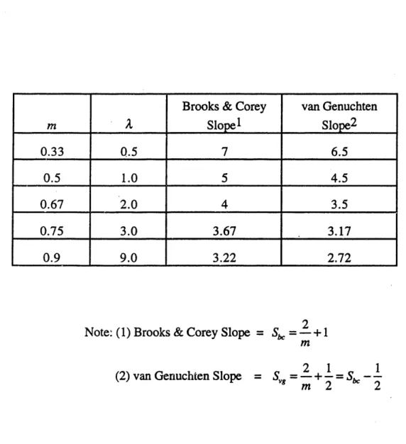
5.1 Unsaturated Hydraulic Conductivity Slope Analysis ... 66
5. 1.1 Compalison Between the Brooks Corey and van Genuchten Models ... 67
5.1.2 Comparison Between the Brooks Corey and Campbell M ethod ... 68
5.2 Results of the Predictive Models ... 70
5.2.1 Criteria for Fit Acceptability ... 70
5.2.2 C ape C od ... 71
5.2.3 H anford ... 72
5.2.5 Las Cruces ... 80
5.2.6 Maddock ... 81
5.2.7 Plainfield ... : ... 81
5.2.8 Sevilleta ... 81
5.2.9 Summary ... 82
5.3 Match Point Selection ... 90
5.4 Leverett Scaling ... 101
Chapter 6 Conclusions ...
109
6.1 Sum m ary ... 109
6.2 Future Research ... Ill. R e fe re n c e s ... 113
Appendix A Table of M oisture Retention Parameters ...
119
Appendix B Cape Cod Curve Fits ... ...
125
Appendix C Hanford Curve Fits ...
134
Appendix D INEL Curve Fits ... 157
Appendix E Las Cruces Curve Fits ...
174
Appendix F M addock Curve Fits ...
180
List of Figures
Figure 1. 1: Typical Moisture Retention Curve ... 1 2
Figure 3 1: Comparison of Moisture Retention Fits Obtained withe(yf) and
i o g YI(e) ... 34
Figure 32: Sensitivity of Calculated Hydraulic Conductivity to Residual Moisture
Content in U niform Sand ... 35
Figure 33: Typical Optimized Parameter Output Box Displayedby KaleidaGraphTm
for a G eneral Curve Fit ... 39
Figure 34: Comparison of the Moisture Retention Fit Obtained Using Different
C onstraints . on es ... 42 Figure 35: Comparison of Estimated Parameter Values for Hanford Sample
2-1636 Using Different Initial Parameter Values ... 45 Figure 36: Comparison of KaleidaGraphTm and RETC Generated Curve Fits for
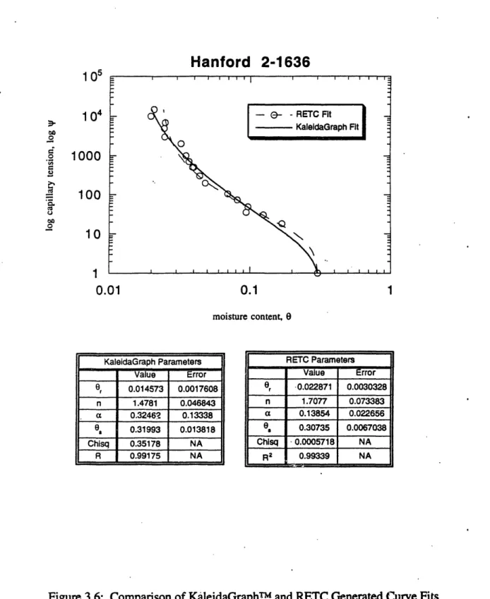
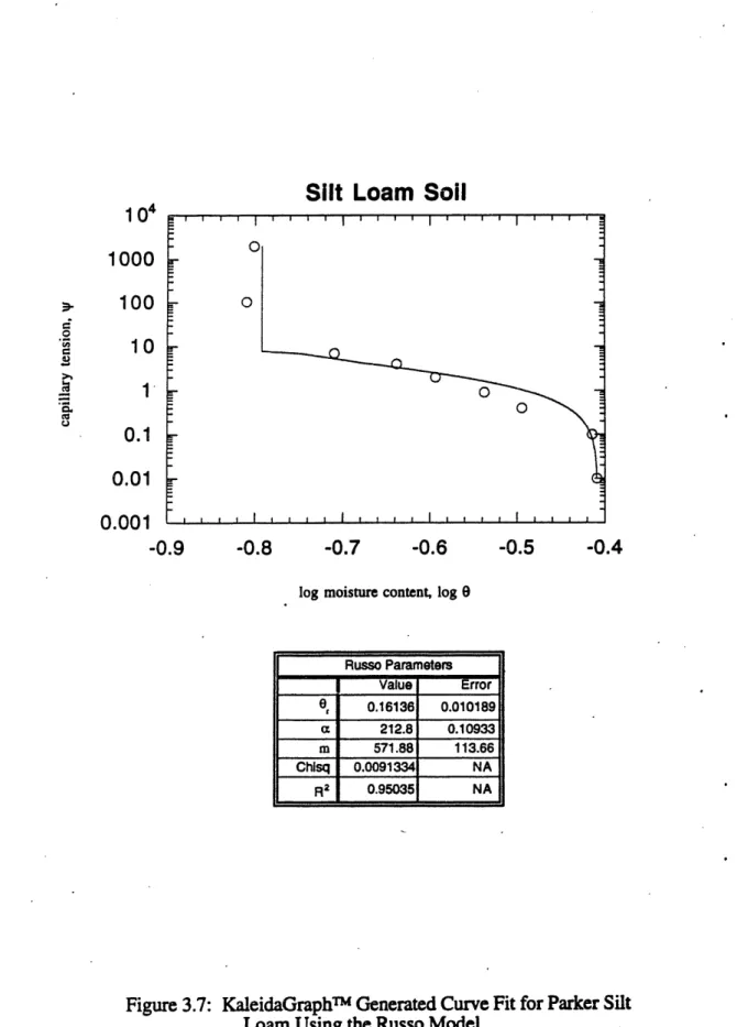
Hanford Sample 21636 Using Different Objective Functions ... 47 Figure 37: KaleidaGraphTm Generated Curve Fit for Parker Silt Loam Using the
R usso M odel ... 5 1
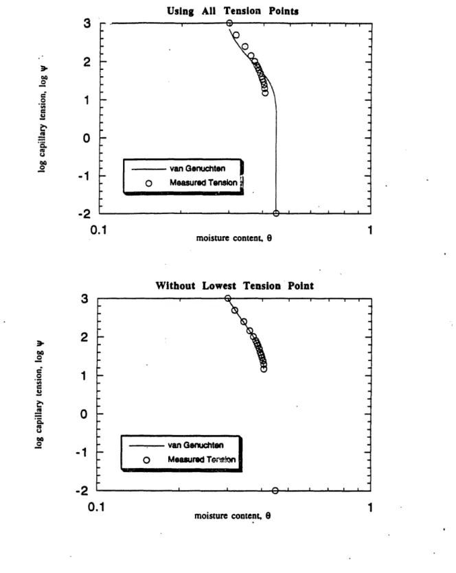
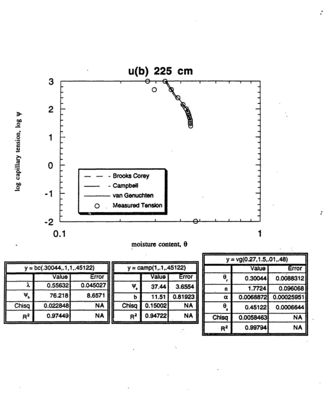
Figure 4 1: (a) Fitted Moisture Retention Curve for R;EL Data Using All Tension Points (b) Fitted Moisture Retention Curve for INEL Data Without the
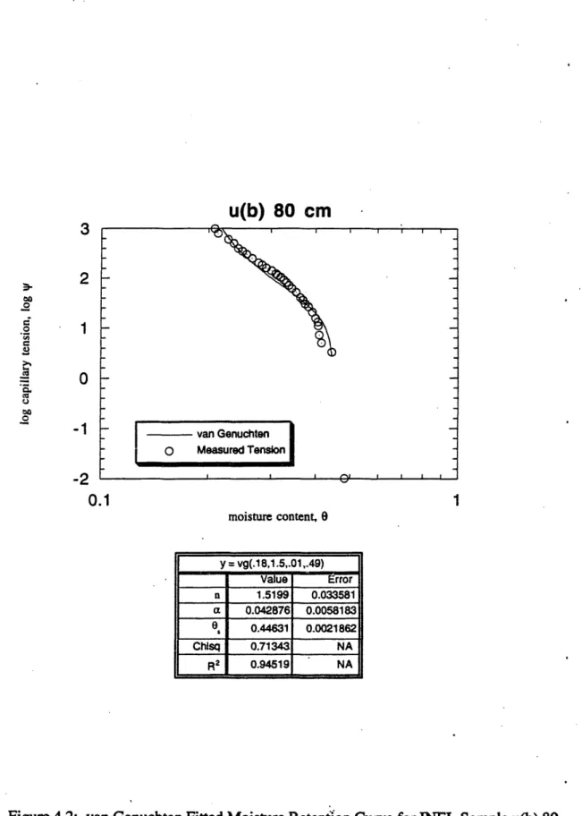
Low est Tension Point ... 60 Figure 42: van Genuchten Fitted Moisture Retention Curve for R4EL Sample ub)
80 cm . ... 62 Figure 43: INEL Moisture Retention Curve Showing Deviation From General
S hape . ... 63 Figure 5. 1: Russo Predicted Conductivity Curve for Cape Cod Core 12a ... 73 Figure 52: Hanford Soil Sample 0079. This sample shows (a) the difference
between SSHC and Ultracentrifuge measured data, (b) measured moisture contents greater than porosity for the ultracentrifuge
measurements, and (c) an example of a good prediction . ... 75 Figure 53: An Example of Scattered Conductivity Data for the Hanford Soils ... 76 Figure 54: Hanford Sample 21639. This sample shows (a) an example of
conductivity data in which K is ill defined and (b) an example of an
Figure 5.5: The Brooks Corey Predicted Slope Compared to the van Genuchten
Predicted Slope ... 79
Figure 56: Mean Error Versus Ks for the Brooks Corey Model ... 83
Figure 57: Mean Error Versus Ks for the Campbell Model ... 84
Figure 5.8: Mean Error Versus Ks for the van Genuchten Model ... 85
Figure 59: Mean Error Versus llylb for the Brooks Corey Model . ... 87
Figure 510: Mean Error Versus llige for the Campbell Model ... 88
Figure 5.1 1: Mean Error Versus a for the van Genuchten Model ... 89
Fiaure 512: Root Mean Square Error Versus lVb for the Brooks Corey M odel ... 9 1 Fioure 513: Root Mean Square Error Versus llyfe for the Campbell Model ... 92
Figure 514: Root Mean Square Error Versus a for the van Genuchten Model ... 93
Figure 5.15: Sensitivity of Calculated Hydraulic Conductivity to Saturated Moisture Content for Uniform Sand ... 95
Figure 516: Regression Slope Versus llVb for the Brooks Corey Model ... 96
Figure 517: Regression Slope Versus IlVe for the Campbell Model ... 97
Figure 5.18: Regression Slope Versus a for the van Genuchten Model ... 98
Figure 519: Graph of n Versus a for the van Genuchten Model . ... 103
Figure 520 (a): Graph Showing the Influence of the van Genuchten parameter n on the Moisture Retention Curve . ... 104
Figure 520 (b) Saled Moisture Retention Curves for Various Values of n at an Effective Saturation Match Point of 13 ... 106
K Figure 52 1: Graph of a Versus I ... 108
List of Tables
Table 2 1: Common Variables and Definitions Found in Unsaturated Conductivity
L iterature ... 19
Table 3 1: Summary of Parameters Allowed for Each Model ... 40
Table 32: Initial Parameter Estimates ... 43
Table 33: Comparison of KaleidaGraphTm and RETC Generated Parameter Values
Using the Same Objective Function ... 4.9
Table 34: Comparison of KileidaGraphTm and Russo Parameter Values ... 50
Table 4 1: Particle Size Distribution and Bulk Density for the Hanford Samples ... 57 Table 5. 1: Comparison of Calculated Slopes Between the Brooks Corey and van
Chapter I
Introduction
1 I Introduction
Numerical modeling is increasingly used to characterize the complex nature of flow and
transport in the subsurface environment. Its use in the characterization of two phase fluid
flow through the unsaturated zone of an aquifer is of particular interest. An accurate
understanding of the flow properties in the unsaturated zone is critical in estimating
contaminant transport, determining soil infiltration, and calculating recharge to the aquifer.
At present, our capacity to create complex subsurface models far exceeds our ability to
characterize the physical system it describes. The accuracy of these models rely heavily on
the quality of the measured data provided. Basic soil properties significantly influence the
outcome of these models.
The unsaturated hydraulic conductivity plays an integral role in determining the
flow characteristics of the unsaturated zone. However, the direct measurement of this.
hydraulic property is often difficult. Typical problems associated with he measurement of
the unsaturated conductivity include high costs, tedious and time consuming measurement
amount of data required to accurately represent the extensive variability of the soil, and the selection. of a measurement technique that can measure conductivity values that span several
orders of magnitude.
These difficulties n the direct measurement of unsaturated conductivity have
prompted the development of empirical models that predict unsaturated conductivity. The
empirical models calculate the relative unsaturated hydraulic conductivity from more easily measured moisture retention and saturated hydraulic conductivity data. Figure 1. 1 displays
a typical moisture retention curve. The predictive models fall under three general
categories: tension dependent models, saturation dependent models, and pore connectivity
models.
Tension dependent models rely on existing measured unsaturated conductivity
values to extrapolate te rest of the conductivity curve. Saturation dependent models
predict the unsaturated conductivity curves based solely on the saturation value, but these
models do not produce unique curves for different soils. Pore connectiviv models predict
the nsaturated conductivity from the measured saturated hydraulic conductivity and
moisture retention data. A specific conductivity curve is generated for each individual soil
type. The goal of this thesis is to assess the performance of four predictive unsaturated
conductivity models derived from the pore connectivity theory.
1. 2 Background
The pore connectivity models relate unsaturated conductivity to moisture retention through
statistical analysis of the pore size distribution. Purcell 1949) and Childs and
10 CZ 4) 4) 6-m U) U) (1) 6. (L Main
Drainage
Curve
31inage
ve iing Is a 1 w nWater Content
among the various models is attributed to differences in the interpretation of pore geometry and the estimate of its contributions to total permeability.
Models based on Purcell's theory view the pores as a bundle of straight capillaries
having a specific radii distribution function. Using Purcell's theory, Gates and Lietz
( 1 950) derive a relationship between the unsaturated conductivity, the capillary tension, and
the moisture content for the wetting phase. Fatt and Dykstra 1951) and Burdine 1953)
modify Purcell to account for tortuosity in the flow path. Burdine also derives a
relationship between conductivity and moisture content for the nonwetting phase.
The Childs and Collis-George (CCG) theory models the flow through the porous
medium as flow through varying pore sizes that are randomly connected at a rejoined
interface. Wyllie and Gardner 1958) derive a relationship between conductivity and
moisture retention by simplifying the CCG theory. They assume that the pores are actually
parallel capillary tubes traversing randomly joined thin layers of soil. Mmilem. applies his
own adjustments to the CCG theory and comes up with a different relationship.
Four closed form analytical unsaturated conductivity models evolve from these,
established pore, connectivity relationships. These models predict unsaturated conductivity
using the measured saturated conductivity and parameters estimated from the moisture
retention data. Brooks Corey 1964) characterize the moisture retention curve as a
power law and apply the Burdine relationship to generate a closed form equation for the
unsaturated conductivity. Campbell 1974) also models the moisture retention curve as a
power law, but applies the Childs and Collis-George relationship. van Genuchten 1980)
represents the moisture retention curve with a mathematical S-shape function and applies
both the Burdine and Mualem relationships to generate two different predictive unsaturated
conductivity equations. Russo 1988) assumes that unsaturated conductivity follows the
Gardner exponential model, a tension dependent model, and backtracks an expression for
There have been many comparisons of these predictive models with measured data.
Stephens and Rehfeldt 1985) evaluate the performance of the van Genuchten model in
predicting the unsaturated conductivity for a fine sand. Measured values of moisture
content and unsaturated conductivity gravitate towards the wet range. The authors
conclude that the van Genuchten approach sufficiently predicts the conductivity for this fine
sand within the measured moisture content regime, but specifically state that predictions
may not be accurate for the dry regions. A few measurements of conductivity and moisture
retention must be made in the dry range before an absolute conclusion can be reached
regarding the overall performance of the van Genuchten model.
Stephens and Rehfeldt also conduct a series of tests to assess the sensitivity of the conductivity predictions to the moisture cntent parameters Or, the residual moisture
content, and Os, the saturated moisture content. Results indicate that the model is highly
sensitive to the value of Or. Predicted conductivities may differ by more than one order of
magnitude depending on the choice of er. The value of Os also influences the predicted
conductivity, but the associated error is not as large as that for Or.
Russo 1988) compares the Brooks Corey, van Genuchten, and Russo model
with two soils, a hypothetical sandy loam and a silt loam. The van Genuchten model
provides the best fit to the measured data. Russo acknowledges that model evaluations
based on just two soils is not sufficient. In order to accurately evaluate wich model works
best, model comparisons based on many ifferent soil types must be erformed.
Keuper and Frind (1 99 1) scale a series of moisture of retention curves for Borden
sands using a modified Leverett scaling relationship. The Leverett concept takes the
various moisture retention curves and scales them into a single curve for all the sand
samples. Keuper et al. use this scaled curve in their numerical analysis to represent the
moisture retention in the aquifer at any single point. A Brooks Corey curve is fitted
through the scaled data. The parameters from the Brooks Corey moisture-retention.
expression are then used to generate an unsaturated conductivity curve. A conductivity
curve is estimated for both the wetting and nonwetting phase from the corresponding
Brooks Corey unsaturated conductivity expression. Numerical simulations modeling
contaminant migration are then carried out in a spatially correlated, random conductivity
field to illustrate the influence of the fluid properties.
Yates et al. 1992) analyzes the van Genuchten model on 36 soil samples taken
from 23 different soils. The soil types range from clay to sands. A majority of the -,Oil
types are fine soils. The analysis compares the measured and predicted conductivity using
the standard van Genuchten predictive method based on a match point at saturated
conductivity, the van Genuchten method with a match point at some selecied unsaturated
conductivity value, the van Genuchten method with an extra f, and two
simultaneous fits with measured unsaturated conductivity data. The authors fnd that the
predictive approach is the least accurate of all the methods and that it introduces a
systematic bias into the unsaturated conductivity estimates. The best fit is obtained by one
of the simultaneous fits. The use of a different match point did not significantly improve
the calculated unsaturated conductivity values. Although the predictive method performed
the worst, Yates et al. stress that this does not invalidate the method. The soils studied in
this analysis do not represent the entire range of soil types. Additional soil types must be
tested before a definitive conclusion can be made.
With the exceptions of Stephens et al. and Keuper et al., all analyses of the
predictive models focus primarily on fine textured materials, such as clays and silts, at a
relatively high moisture content > 10%). Khaleel et al. specifically looks at the
Hanford sands. The highly heterogeneous Hanford sands contrast nicely with the
homogeneous sands previously studied. Khaleel et al. conclude that the van Genuchten
predictive method shows noticeable deviation from the measured values, especially at low
moisture contents. The use of a different conductivity match point from the unsaturated
conductivity region results in an improvement.
1.4 Thesis Objectives
The specific objectives of this study are the following:
• To evaluate the perfon-nance of the Brooks Corey, Campbell, Russo, and van
Genuchten models in predicting the unsaturated conductivity of aquifer-like
materials at low moisture contents.
• To assess the influence of changing the match point for these models.
• To investigate the concept of Leverett scaling.
1.5 Thesis Outline
This thesis is organized into six chapters. Chapter 2 summarizes the various types of
unsaturated conductivity models and presents a detailed description of the four models used
in our analysis. Chapter 3 concentrates on the curve fitting methodology. In Chapter 4,
the data selection process is discussed and a brief description of each data set is presented.
Chapter analyzes the curve fitting results. Chapter 6 presents the conclusions and
Chapter 2
Unsaturated Hydraulic Conductivity
Aodels
This chapter summarizes the various types of models used to calculate unsaturated
hydraulic conductivity. This review follows the format presented by Mualem 1986).
Section discusses the variables and definitions commonly found in unsaturated
conductivity equations. Sections 2 3 and 4 present the different categories of conductivity
models, namely tension dependent models, saturation dependent models, and pore
connectivity models. Section discusses coupled moisture retention/unsaturated
conductivity models that predict unsaturated conductivity using only measured saturated
hydraulic conductivity and moisture retention data.
2.1 Relevant Notation and Definitions
Unsaturated conductivity models attempt to predict conductivity values through measured
lists standard variables and definitions that appear ubiquitously in the unsaturated
conductivity literature.
2.2 Tension Dependent Models
When supplied with an incomplete set of unsaturated conductivity data, capillary tension
models provide a relatively straightforward and simplistic way to estimate the unknown
unsaturated conductivity values. Capillary tension models rely on existing measured
conductivities to systematically extrapolate the rest of the conductivity curve for any known
tension.
Application of the models serves multiple purposes. Use of these models can
minimize the number of measurements required for adequate representation of actual field
conditions. They also provide closed form analytical equations used to solve unsaturated
flow problems. In addition to saving time and improving accuracy, a closed form solution
simplifies the computational procedure used in numerical simulations.
One of the earliest and most widely used unsaturated hydraulic conductivity models
is formulated by Gardner 1957):
K,(V = exp(-ayf) (2.1)
where
a = an empirical soil parameter
Gardner derives this analytical equation relating unsaturated hydraulic conductivity to
capillary tension as a plausible solution to Richard's Equation 193 1) for a steady state flow
Standard Definitions K = K K, = O 0) 1 (01 - 01) Standard Variables
e actual water content
er residual water content es saturated water content V capillary pressure
K unsaturated hydraulic conductivity
Ks saturated hydraulic conductivity
Kr relative hydraulic conductivity
S saturation
Se effective saturation
Table 2 1: Common Variables and Definitions Found in Unsaturated Conductivity Literature.
general values may be used to obtain a rough estimate of the hydraulic conductivity when
no data are available.
This exponential model is frequently employed by many soil scientists because of
its simple form. Recent research involving the stochastic analyses of steady and transient
unsaturated flow in heterogeneous media (Yeh et al., 1985; Mantoglou and Gelhar, 1987)
have adopted the Gardner exponential model to represent the local unsaturated hydraulic
conductivity.
Although simplistic in nature, the Gardner exponential model does have certain
limitations. The model does not hold well over a wide range of values. Hence, the
equation is valid only for a limited range of values of capillary tension.
Brooks and Corey 1964) suggest an alternate analytical form relating the
conductivity to capillary tension
_n
K, for <
K = K, for >
where
Yfcr an empirically determined critical capillary tension value
n a soil determined empirical parameter
This power law model is extremely popular in the petroleum industry.
Obvious shortcomings of the Brooks and Corey model include its high degree of
non-linearity and its inherent discontinuity near the critical capillary tension point. This
poses a distinct problem for numerical models that simulate fluid flow in the unsaturated
zone and makes it very difficult to deal with analytically. The discontinuity in the slope can
Other exponential (Rijtema, 1965) and power law (Wind, 1955) models have also
been proposed. The parameters for these formulas differ slightly from Gardner and
Brooks and Corey. These formulas have not found the same degree of wide acceptance
and usage as the two models previously discussed. Tension based models also take on
other mathematical forms. For example, King 1964) proposes a model using the
hyperbolic cosine function.
2.3 Saturation Dependent Models
Models in this category stem from the assumption that flow through the unsaturated porous
media resembles aminar flow through a capillary tube. By assuming this capillary tube
concept, the saturation based models are able to represent the microscopic flow through the
porous media by macroscopically measured flow parameters, such as hydraulic
conductivity and average velocity. Equations, such as the Hagen-Poiseuille, that link the
microscopic level to the macroscopic level form the theoretical basis behind these models.
Saturation dependent models are convenient, but they do not produce unique conductivity
curves for different soil textures.
Averjanov 1950) views unsaturated flow as flow in parallel, uniform, cylindrical
capillary tubes. The wetting fluid forms a homogeneous film along the cylinder wall,
whereas the nonwetting fluid occupies the central portion of the tube. Based on these
limiting conditions, the following relationship between unsaturated conductivity and
saturation is derived:
Yuster 1951) essentially solves the same equations as Averjanov, but imposes
slightly different flow conditions. Yuster assumes that the nonwetting fluid in the center of
the tube flows under the same gradient as the wetting fluid. The solution is also in a power law form, but the exponent varies:
Kr Se 2.0
Kozeny 1927) develops a model for saturated hydraulic conductivity assuming
flow through spherical porous media:
K
= 9 2 03CvA' (2.2)
where
g = gravity acceleration
v = kinematic viscosity
As = solid surface area
C = flow configuration constant
Irmay 1954) generalizes Equation 22 to represent flow through unsaturated porous media. Since the actual values of As and C are impossible to accurately determine,
Irmay suggests that Ks act as a substitute for As and C. This yields:
Kr =Se 3
Brooks and Corey 1964) observe that Avedanov's relationship seems to agree
over a larger variety of soils than Irmay. From the above equations, one can obviously see
the equation exponents. This indicates that K values may be influenced by the flow
conditions.
Mualem 1978) makes an interesting modification-to the macroscopic concept by
choosing a slightly different approach. Once again, a general power relationship is
assumed:
Kr = Sen
where
n = a soil parameter
Mualem attempts to detem-ine the value of n by matching the equation to experimental data
for 50 different soils. No single optimal value for n is found. Instead the analysis
indicates that a large range of possible values for n exists. Values for n span a lower limit
of 2.5 to a fairly high value of 24.5 for fine textured soils. Instead of fixing the exponent n
as a constant, Mualem defines it as a soil water characteristic parameter.
Statistical analysis of the retention data obtained from the 50 soils exhibit a
correlation between the soil parameter, n, and the energy associated with the wilting point,
W:
0
w y. Vd 0
where
W the energy required to drain a unit bulk volume from saturation
to the wilting point at W 15000 cm
7W the specific weight
Using available moisture retention data, Mualem plots n versus w and derives an
n = 30 + 0.015 w
Mualem tests this model and finds good agreement between the measured and predicted
conductivity values.
2.4 Pore Connectivity Models
Pore connectivity based models relate unsaturated hydraulic conductivity to moisture
retention and saturated conductivity measurements through statistical analysis of the pore
size distribution. The purpose of these models is to predict the conductivity curve from
measured moisture retention and saturated conductivity data. No actual measurements of
unsaturated conductivity are necessary.
Models in this category regard the porous medium as a set of randomly distributed,
interconnected pores. The moisture retention curve is viewed as the pore radii distribution
function. Flow in the porous media is controlled by the statistical probability of the random
pores connecting. Models primarily differ in their interpretation of the pore geometry and
the estimate of its contribution to total permeability. Models either regard the pores as a
bundle of capillaries or as random connections located at a rejoined cross section.
2.4.1 Capillary Tube Models
Purcell 1949) models the pores in soil as a bundle of parallel, straight capillary tubes.
Gates and Lietz 1950) apply the Purcell theory and establish the following relationship
between conductivity, capillary tension, and moisture content:
i de
fo 2
0) V
Kr dO
Fatt and Dykstra (1 95 1) modify the above equation by accounting for tortuosity in
the flow path:
de
(0) fo ""' 2+b
0 de
fo, V 2+b
The tortuosity factor, b, varies for different soil types.
Burdine 1953) also modifies Gates and Lietz, but use a different tortuosity
relationship. The tortuosity correction factor selected is the square of the effective
saturation.
de
fo, 2 0 - S2 0 K, e. d (2.3) fo, V2Burdine applies the same capillary model to derive a complimentary relationship for the nonwetting fluid, Kmw,
de
K,... (9 = (I S) 2 Vf 2 (2.4)
de
fo, - V2
Experimental results show good agreement between measured and predicted values using
the Burdine relationships.
2.4.2 Rejoined Cross Section Models
Childs and Collis-George 1950) model flow through a porous medium as flow through
varying pore sizes that are randomly connected at a rejoined interface. The flow is
sequence contribute to the overall conductivity. Only a single connection exists between
the pores. Various other investigators (Millington and Quirk, 1961; Jackson et al., 1965;
and so forth) have tested this theory and have modified it.
Wyllie and Gardner 1958) simplify this theory by assuming that the porous
medium is made up of randomly joined thin layers traversed by parallel capillary tubes.
The flow is controlled by the interface between the layers.
Mualem 1976) applies the Childs and Collis-George theory and arrives at the
following relationship: 0 dO fo, (2.5) K (0) = S 011 dO f V
Mualem tests this relationship on 45 soils and concludes that the optimal value for n is 0.5.
2.5 Coupled Moisture Retention and Unsaturated
Conductivity Models
This section reviews four coupled moisture retention/unsaturated conductivity models.
These models propose a mathematical equation for the moisture retention curve, apply the
equation to a pore connectivity model, and then provide a closed form analytical solution
relating the unsaturated conductivity to moisture retention and saturated conductivity. The
advantage of these models is that they can predict the unsaturated conductivity from more
easily measured moisture retention and saturated conductivity values. This thesis will
focus on how well the Brooks Corey, Campbell, and van Genuchten models can predict
unsaturated conductivity. The Russo model is also analyzed, but the data available for this
2.5.1 Brooks
Corey
Brooks Corey 1964) characterize the moisture retention curve as a power law
relationship:
A
Vb
S" for V > V (2.6)
where
pore size distribution index
y1b capillary tension at the bubbling pressure
The bubbling pressure is related to the maximum pore size forming a continuous network
of flow channels within the porous medium. Brooks Corey 1964) substitute their
moisture retention equation into Equations 23 and 24, resulting in an explicit equation
relating the moisture retention and saturated conductivity to the unsaturated conductivity.
Solutions for both the wetting and nonwetting phase are derived. The wetting phase
relationships are: 2+3A (2.7) K = S,) for ig Vfb 2+3A K - Vb (2.8) V
The nonwetting relationships are:
2+2, (1 Se )2 -Se (2.9) for igb A 2 - 2+1 Vb '9b (2.10) V - - V
2.5.2 Campbell
Campbell 1974) represents the moisture retention curve by
Vf, 0 (2.11)
0.1
where
Nfe the air entry water potential
b an empirically determined constant
The Campbell equation differs from Brooks Corey. First, Campbell assumes that there
is no residual moisture content. Second, the Campbell equation is valid for values of
tension below the bubbling pressure.
Campbell applies the Childs and Collis-George model and derives a conductivity
retention relationship for the wetting phase only.
2b+3 K, 0 (2.12) e., + 2 K, Ve b (2.13) V
Near saturation, Equation 211 faces a sharp discontinuity. This break in the retention
curve is a result& the gradual entry of air near the saturation region. Clapp and
Hornberger 1978) suggest a modification to the moisture retention equation to account for this discontinuity. At the inflection point (Si, Vi ) of the moisture retention curve near
saturation, Equation 2 1 1 is replaced by a parabolic expression
Vf = -m(S - n)(S - 1) for Si S5 1 (2.14)
e
S =:e,
M
Vi Vib (I T Si 1 Si n 2S - Vb 1 MsiEquation 214 passes through the point (Si VIi and (1,O) and the derivative, d Vf IdS of
both Equations 211 and 214 are equal at the inflection point.
2.5.3 Russo/Gardner
Russo 1988) assumes that the relationship between conductivity and capillary pressure
follows the Gardner exponential model (Equation 2 1). An accompanying equation for the
moisture retention curve is derived by selecting Gardner's conductivity relationship as a
closed form solution to Mualem's model (Equation 25) and backing out a relationship
between saturation and capillary tension.
2 Se (e -0.5aW (i+0.5aV (m+2) (2.15) where
a
theGardnerempir.calparameter
m 2n(nisanempiricalparameterinMualem'smodel)2.5.4 van Genuchten
van Genuchten 1980) represents the moisture retention curve with
M
where
a, n, m =empirical parameters
van Genuchten substitutes this equation into Mualem's model (Equation 25) and solves.
A closed form analytical solution is obtained when the constraint in = - l1n is imposed.
Solutions for the wetting phase are derived:
M-2 K,=S,2 I- I- SM (2.17) when m=l- 1 n 1 (aVy-l [1 + ,,,)n ]-,n (2.18) K, M + (aV)' 2
Parker et al. 1987) derive the nonwetting solution:
M-2
1 1
11111 = - S, 2 -SIM (2.19)
van Genuchten also derives relationships between the conductivity and the moisture
retention using Burdine's theory (Equation 24).
M K, (S., 21 1 SIM (2.20) 2
when
m=l--nK,
+
(2.21)
11+ (,,),j2mM
K.. =
(I e)2 I - SIM(2.22)
At high tension, where ayl)n >> 1, the van Genuchten/Burdine combination becomes the
Brooks Corey model. Since we are already evaluating the Brooks & Corey model, our
analysis of the van Genuchten model will focus only on the van Genuchten/Mualern
Chapter 3
Curve Fitting 1\4ethodology
This chapter describes the curve fitting technique applied to generate the moisture retention
parameters used in predicting the unsaturated hydraulic conductivity. The first section
discusses the use of a nonlinear optimization procedure, its key parameters, and the initial
values used for the parameters. The second section presents the model calibration process.
The third section details the procedure used to select valid data points for the Brooks
Corey model.
3.1 Curve Fitting Technique
The data analysis/graphics application program KaleidaGraphTM provided the analytical
means to evaluate the moisture retention data and produce the optimal values for the fitting
parameters. The general curve fit function in KaleidaGraphTM allows the user to define a
general form equation and its determining parameters. The program then applies a
nonlinear least-squares optimization procedure to the data values and generates the optimal
performed using the Levenberg-Marquardt algorithm. This program presents a powerful
and effective technique for performing data analysis.
3. 1.1 Nonlinear Optimization Function
As mentioned i Chapter 2 our assessment of two phase flow characterization of soils will
focus on four coupled moisture retention/unsaturated hydraulic conductivity models. We.
are interested in how well these models can predict unsaturated hydraulic conductivity
using only moisture retention data. The models are the Brooks Corey/Burdine model,
the Campbell model, the Russo/Gardner model, and the van Genuchten/Mualem model
(with m = - n).
The analysis focuses on the low moisture content region of the moisture retention
curve. We are primarily interested in the ability of these predictive models to accurately
assess the unsaturated hydraulic conductivity of the vadose zone in an aquifer. Typical
moisture contents found in the vadose zone are in the low moisture regime of the moisture
retention curve. This regime is characterized by low unsaturated hydraulic conductivity.
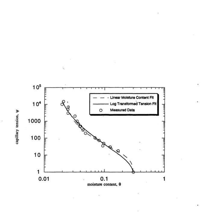
Selecting the form of the defining equation in our general curve fit will affect the optimization process. If we define the moisture retention equation in terms of O(V) and
optimize on a linear scale, we lose resolution of the moisture retention curve at low
moisture contents (Figure 3 1). The residual moisture content for sand and other coarse
soils is typically just a few percent of the saturated water content. By using a inear scale to optimize e, the low moisture content values might simply be relegated as error. This will
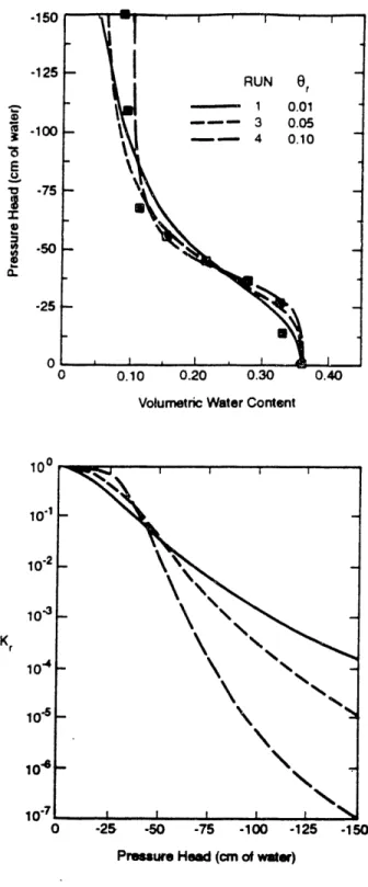
result in an inaccurate value for the residual water content. Stephens et al. 1985) show
that the value of the residual moisture content has a significant influence on the shape of the
predicted hydraulic conductivity curve near the low conductivity region (Figure 32).
05
04
I I . . . 1:
- - Unear Molsture Content Fit
I
Log Transfoffned'Tension Fit
-0 Measured Data
0
-. . I . I . I I I . . . . C .2 'A C P >1 I w U 1000 100 1 0 1 I -0.01 0.1 moisture content, 1-150 -125 2M -a E 2
I
0 zfie 9 a. -100 -75 .50 -25 0Volurnetric Water Content
- A
Kr
0 -25 .50 -75 -100 -125 -150 Pressure Head (crn of water)
Figure 32: Sensitivity of Calculated Hydraulic Conductivity to Residual Moisture Content in Uniform Sand. (From Stephens et al., 1985)
Defining the moisture retention equation in terms of VO) enables the optimization
process to emphasize the high tension/low moisture content region. This meets our
primary objective of highlighting the low moisture content region. However, in doing so,
it tends to neglect the fit near the low tension/high moisture content region. On a linear
scale, the measured tension data span up to four orders of magnitude. This wide range of
values makes it difficult to accurately optimize the retention curve at low tension values. Selection of a logarithrnically transformed scale for Ve) allows us to emphasize the
low moisture content range, yet still provide a reasonable fit in the high moisture content
region (Figure 3 ). By implementing the log transformed scale, tension values are
reduced to the same order of magnitude. The curve fit procedure minimizes the relative
error between data points on a log scale as oppose to minimizing the absolute error on a
linear scale. The error values will be more uniform over the entire range of tension and will provide a more accurate representation of the data.
The following form of the moisture retention equation for each model is used in the
optimization procedure:
Brooks Corey
log Y/ = log log for Vf > V, (3.1)
Campbell
Russo (3.3) van Genuchten I
logv=
(3.4)a
The KaleidaGraphTm general curve fit employs a nonlinear least-squares
optimization procedure to minimize an objective function. For the Brooks Corey,
Campbell, and van Genuchten models, the objective function, O(b), has the general form:
(3.5) where
N
Wi log Vi 15g yf (b) b= the number of moisture retention data in the sample = weighting coefficients for a single data value
= the log of the measured tension value
= the log of the calculated tension value = the model parameter vector
The Russo/Gardner model objective function has the form:
(3.6) log = log 0, (O., 0')(e -0.5aV (I 0. 5 aip)) m+2
N 2 O(b = I Wi [log V - 6g VI b)]l i=1 N 2 O(b = I w, [log O - 6g e (b)]J i=1
where
N = the number of moisture retention data in the sample
Wi = weighting coefficients for a single data value
log ei = the log of the measured content value
16g e (b) = the log of the calculated water content value
b = the model parameter vector
The weighting coefficient is used to place more or less weight on a single data value
based on a priori information regarding the reliability of the data point. In all of our
analyses, the weighting coefficient was set to unity.
The model parameter vector, b, contains the unknown coefficients in our general
equation. In the nonlinear least-squares optimization process, the parameters are adjusted
until a local minimum value of squared error is found. A more detailed discussion of the
model parameters is presented in a later section.
All algorithms and equations used in the calculation of the general curve fit can be
found in the book Numerical Recipes in C by William H. Press, Brian P. Flannery, Saul A. Teukolsky, William T. Vetterling, Cambridge University Press (KaleidaGraphTm
reference guide).
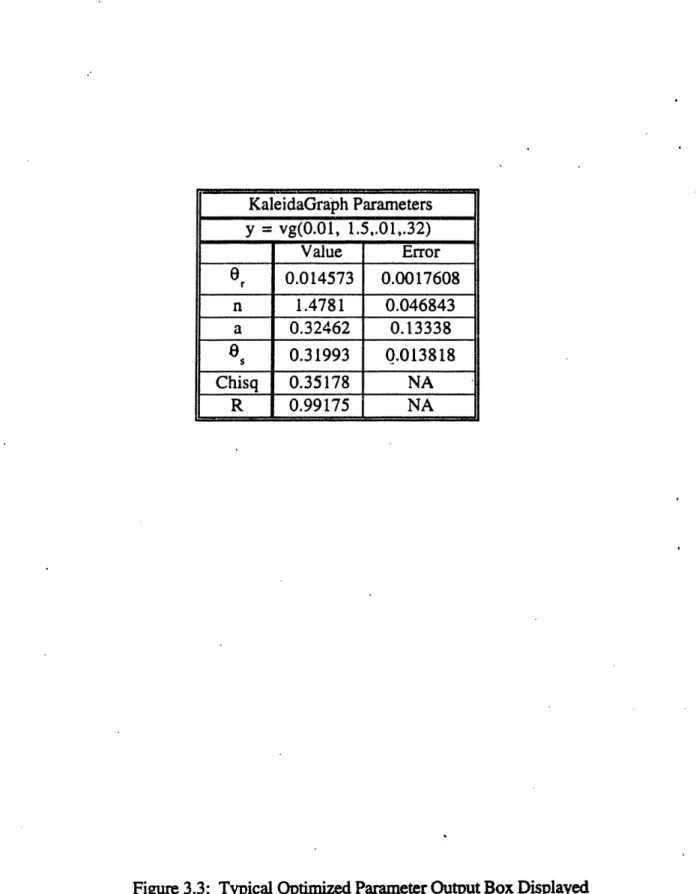
3.1.2 Optimization Output
Once the curve fit optimization is finished, KaleidaGraphTm generates a fitted curve through
the data points and displays an output box that contains the optimized equation parameters
(Figure 33). In addition to the parameter values and its associated error, tb..e box also
shows the initial estimates for the parameters, the sum of the squared errors,' 2 and the
value of either R or The sum of the squared error is calculated using the general
KaleidaGra:ph Parameters = g(O.01, 1.5,. 01,32) Value Error 0r 0.014573 0.0017608 n 1.4781 0.046843 a 0.32462 0.13338 as 0.31993 0.013818 Chisq 0.35178 NA R 0.99175 NA
Figure 33: Typical ptimized Parameter Output Box Displayed by KaleidaGraphrm for a General Curve Fit.
Model Parameters
Brooks & Corey Or, b
Campbell Ve, b
Russo Or, Os, cc
van Genuchten 11 Or, Os, n, rn a
Y,
- f (xi)'
a,
2
where
the measured value the calculated value the weight
of the weight is set at unity.
Yi
f(Xd ai
In our analysis, the value
3.1.3 Model Parameters
The model parameters for the moisture retention curve varies from model to model. Table
3.1 lists the parameters allowed for each model.
Table 3 1: Summary of Parameters Allowed for Each Model. (Note: The parameters m and a are not the same
between the Russo and van Genuchten models)
In the van Genuchten analysis, the restricted case where m = - 11n is selected
because it provides a simple, closed form analytical expression for the unsaturated
hydraulic conductivity. Hence, m is no longer a parameter in our optimization process for
the van Genuchten model.
N
X2=
I
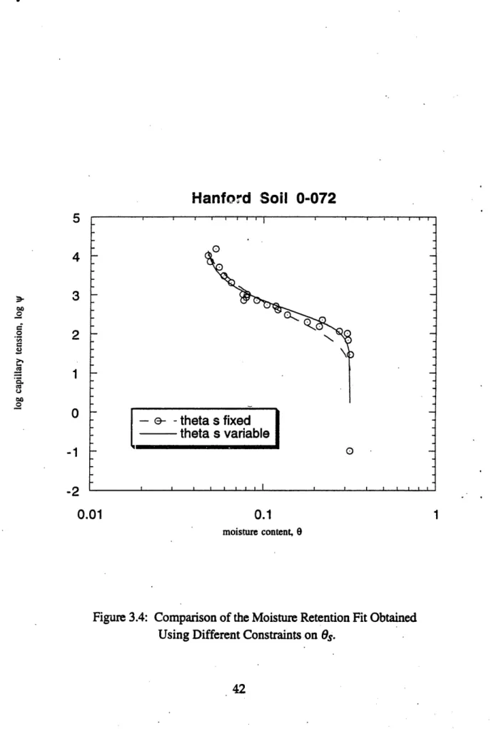
In some instances, the parameter Os in the Russo and van Genuchten models is set equal to the measured soil porosity. Selecting a fixed value of Os is desirable when there is
insufficient data on the moisture retention curve to define a reasonable value. In the situation here we have a well defined moisture retention curve, choosing Os as an
optimized parameter for the van Genuchten model will result in a more accurate definition
of the sharp downturn in the moisture retention curve near the saturation region. In general, KaleidaGraphTM was allowed to determine the optimal value of es whenever
possible. Figure 34 illustrates the noticeable difference in the moisture r.ention fit acquired for the Hanford soil sample 0072 with different es constraints.
Modifications to the parameter are necessary for ill defined moisture retention curves. For some data sets, the values of Or or Os had to be defined. The optimized values
for these data sets did not provide reasonable values for these parameters. Negative values
of Or and values of Os greater than unity are obtained in these cases. The following chapter indicates the data sets that require modifications to the parameters.
3.1.4 Initial Parameter Estimates
The nonlinear optimization process requires the user to specify initial estimates of the
parameter values. These initial guesses are used to generate the optimal parameter values.
It is crucial that reasonable expected values of the parameters are specified. Initial values
are chosen from suggested values found in recent literature (Khaleel et. al, 1995 and Russo, 1988). The initial values vary from soil to soil. Different initial values for Or and
a are chosen depending on its textural classification. Compared to finer soils such as the
silts, sands generally have smaller initial guesses. For the soils where the moisture
. - . . I - 1 -9
theta s fixed
theta s variable
4 f I . . . I , I - - - I - I - . - I I . . . 5 4 I I . I . . I . In
3 3-00 Q CF .2 Q co Q w .2 2 1 0 -1 -2 0 0.01 0.1 moistwe content,Figure 3A Comparison of the Moisture Retention Fit Obtained
Using Different Constraintson Os.
-1
Models Initial Parameter Estimates
Brooks Corey Or (sand)= 0.01
Or (silt)= 0. 1 = 0. 1 W = Campbell We = b 0. 1 Russo Or 0.01 Os porosity M oc
van Genuchten Or (sand) = 0. I
Or (silt)= 0. 1
Os porosity
n 1.5
(X and)= 0.00 1
cc (silt)= . I
last measured moisture content value are selected. Table 32 lists the initial values generally
used for each model.
3.1.5 Sensitivity of Initial Parameter Estimates
To test the sensitivity of the optimization process to the initial parameter estimates, the
fitting procedure is performed on the same sample for different initial values (Figure 35).
For well defined moisture retention curves, the difference is negligible. For ill defined
moisture retention curves, the resulting values for Or or Os are arguably much more
sensitive to the initial specified values. In these cases, the initial value for Or is either
visually estimated from the moisture retention graph or fixed at a value deemed reasonable
for a similar soil texture. An initial guess for Os near porosity is usually sufficient to
produce a reasonable value for Os. In a few cases, the parameter Os had to be fixed.
3.2 Model Calibration
Khaleel et al. 1995) uses the computer program RETC (Leij et al., 1991) to evaluate the
performance of the van Genuchten model for the Hanford soils. RETC is a nonlinear, least
squares curve fitting procedure that optimizes specified model parameters for nonlinear
equations with multiple parameters. Our analysis uses the program KaleidaGraphT in
place of RETC.
Russo 1988) derives the Russo/Gardner model and fits it to two distinct soils, one
hypothetical and one actual. The following sections illustrate the differences between our
y = vg(.018,1.7080,.1385,.30) y = vg(O-01 15,01,32)
Value Error Value Error
0
r0.014573 0.0017608
0
r0.014573 0.0017608
n 1.4781 0.046843 n - 1.4781 0.046843-Oc
0.32462
013338
a
0.32462
0.13338
0.31993
0.013817
0
0.31993
0.013818
S SChisq
0.35178
Chisq
0.35178
NA
R 0.99175 N R 0.99175 - NAHanford 21636
van Genuchten Curve Fit
Figure 35: Comparison of Estimated Parameter Values for Hanford. Sample 21636 Using Different Initial Parameter Values.
3.2.1 RETC
RETC is a versatile computer program capable of finding the optimal parameters for the van
Genuchten and Brook & Corey models under varying parameter constraints. The program
allows the model parameters to be determined by using only moisture retention data or both
measured moisture retention data and unsaturated conductivity data. RETC optimizes an
alternate form of the van Genuchten equation:
0=0
(Os L
r 11 + ayf), IM
with the objective function
N 2 M 2
00 5) IWi[O - b(b)]
I
W.W2w,[Y - i(b)]J i=,V+lwhere
Oi the measured moisture content
Oi the calculated moisture content
Yi the measured unsaturated hydraulic conductivities
Yi the calculated unsaturated hydraulic. conductivities
b the parameter vector
N the number of moisture retention data
M total number of measured data (retention and conductivity)
W1, W2 weighing factor between retention and conductivity data
Wi weighing factor for a single data point
The RETC objective function optimizes O(Vf), whereas the defined KaleidaGraphrm
objective function (Equation 35) optimizes log VO). Use of different objective functions
Hanford 21636
I I I I . I ' ' I I I I . I . I 1 RETC Fit KaleldaGraph Fit 0 RETC Parameters Value - - Error 0r -0.022871 0.0030328 1.7077 0.073383 a 0.13854 0.022656 es 0.30735 0.0067038 Chlsq - 00005718 NA R2 I 0.9m I NA KaleidaGraph Parameters Value Error 0r 0.014573 0.0017608 n 1.4781 0.046843 1 ot 0.32461 0.13338 es 0.31993 0.013818 Chisq 0.35178 NA 0.99175 1 NA 05 04 1000100
1 0 to .2 d .Iwr-q M U 00 0 1 0.01 0.1 1 moisture ontent 0
Figure 36: Comparison of MeidaGraphTl and RETC Generated Curve Fits for Hanford Sample 21636 Using Differ-&it Objective Functions.
parameters generated by the two varying functions for the Hanford sample 21636.
Parameter values for the RETC curve fit are taken from Khaleel et al. 1995).
The van Genuchten parameters generated by the two methods differ slightly. The
parameters vary because the emphasis of the governing equations differ. The
KaleidaGraphTm analysis focuses on the low moisture content region by optimizing with
respect to log V/. RETC optimizes 0, thus concentrating on the high moisture content
region. The difference in regional emphasis is apparent in Figure 36.
To compare the optimization ability of KaleidaGraphTm against RETC, the RETC
objective function is entered into KaleidaGraphTm and a fitted curve is generated for
Hanford sample 21636. Results from this test present a form of model calibration. If
KaleidaGraphTM is comparable to RETC, the generated parameter values should be the
same. RETC parameter values are taken from Khaleel et al. 1995). As seen in Table 33,
the optimized parameter values are essentially the same.
3.2.2 Russo/Gardner
To calibrate the Russo model, data for the Parker silt loam soil is read off the graph in
Russo 1988). An optimization is then performed on the measured data using Equations,
3.3 and 36. The purpose of this analysis is to replicate Russo's parameter values for this
soil. Table 34 compares the KaleidaGraphTm generated results versus the Russo values
found in the literature. As seen in Figure 37, the fitted curve does not accurately represent
the measured data. Significantly different parameter values are generated in our
optimization process. Results vary because Russo uses additional data to constrain the
parameter search. Russo's objective function is
N 2
0(b)=EJwJQ(tj)-(tjb)]J
+JV[0(k5)-b(k5,b)]12Parameter KaleidaGraphrm RETC
Or 0.022871 0.023
n 1.7077 1.7080
a 0.13854 0.1385
es
0.30735 0.3073Table 33: Comparison of KaleidaGraphrm and RETC Generated Parameter Values Using the Same Objective Function.
Parameter KaleidaGraphrm_ Russo
Or 0.16136 0.186
a (M- 1) 2.128 4.995
I M 1 571.88 1 0.021 i
Slit Loam Soil
- - - . . . . Russo Parameters Value Error Of 0.16136 0.010189 Q 212.8 0.10933 M 571.88 113.66 ChIsq 0.0091334 NA R 2 0.95035 NA 041000
100 ci .21In C 2 >1 I9 M IV U 1 0 1 0.1 .9 0.01n MI
W. J I -0 -0.8 -0.7 -0.6 -0.5-0.4
log moisture content, log
Figure 3.7: KaleidaGraphrm Generated Curve Fit for Parker Silt Loam Using the Russo Model.
where
Q(t i the set of cumulative outflow measurements at specified
times ti
(tj, b) = the numerically calculated value of the outflow
corresponding to the trial vector of parameter values, b
O(k5) = the measured moisture content at h 15,000 cm H20
0(451b) = the predicted moisture content at h 1 5,000 cm H20
Wi = weighing factor
V = weighing factor
The parameter values from KaleidaGraphTm might have reproduced Russo's values if extra
constraints had been added.
3.3 Data Validation Procedure for the Brooks
Corey
Model
The Brooks Corey moisture retention relationship was discovered by plotting log S, as a function of log y/. The resulting graph of the log transformed variables is a straight line
with the negative slope, A. The Brooks Corey theory holds only for values of tension,
yf, greater than or equal to the tension at the bubbling pressure, V. In order to obtain a
proper fit to the model, points near saturation that are below the bubbling pressure tension
are not included in the curve fitting procedure.
Since the bubbling pressure tension and the residual water content are parameters in
the optimization process a graph of log S, versus log yf is not possible. A method used to
points in determining the slope and bubbling pressure tension value. An assumption is
made that e, is relatively small compared to the measured values
of
e. A graphof og e
versus log V/ is generated to represent the graph of the log S, versus log iy. In accordancewith the original Brooks Corey method, a straight line is drawn through the data points.
Any data point near saturation that deviates from the general linear trend is excluded from
Chapter 4
Data Description
A total of 71 soil samples, supplied from seven data sets, is analyzed. The first section in
this chapter details the criteria used to select the data sets. The second section briefly
describes each data source, mentions the techniques used for data measurement, and
discusses any modifications made to the curve fitting parameters.
The computer disk accompanying this thesis contains the measured values of
moisture retention and unsaturated conductivity used in the analysis. AR files are saved as
Macintosh tab delineated text ffies. Each soil type has an individual file. The soil sample
number is located in the fst column of the file.
4.1 Data Selection Process
The primary purpose of the analysis is to assess the ability of these predictive models to
accurately characterize the unsaturated conductivity in aquifer like materials. Typical
aquifer materials consist of sandy, coarse soils. The relatively dry vadose zone located just
sets emphasizing these properties are selected. The data consists primarily of measured
moisture retention and unsaturated conductivity values obtained from sands and sandy loam
material. The Hanford data set measures capillary tension up to extremely high values,
thus giving a detailed picture of the low moisture content region.
A secondary purpose of the data selection process is to choose data sets that indicate
some measure of consistency to the fitting process. Data sets that contain multiple samples
from the same aquifer provide the repetition needed to search for consistent trends. All data.
samples in a single data set are measured by the same techniques and by the same
individuals. Thus, differences between the soil samples cannot be attributed to differences
in the measurement techniques. This gives us a good indication of the soil variability in
aquifer soils. Soil samples from the same aquifer also represent a collection of similar soils
of varying pore size distributions and saturated conductivity values.
4.2 Data Sources
This section provides a concise summary of the site description, the experimental
procedures used to measure the data values, and the changes made to the curve fitting
parameters. For more detailed information regarding the site characterization and
measurement process for each site, the reader is advised to refer to the referenced papers.
A thorough summary of current laboratory and in-situ field measurement techniques for
moisture retention and hydraulic conductivity can be found in Hillel 1980) and Stephens
(1996).
4.2.1 Cape Cod Data Set
Soil samples from this set are taken from a glacial aquifer located on Cape Cod,
that was deposited during the retreat of the continental ice sheets from southern New
England about 12,000 years ago (LeBlanc et al., 1991). This aquifer is the primary source
of freshwater for the inhabitants of Cape Cod and all its visitors. At present, the site is
contaminated by several pollutant plumes which threaten the underlying aquifer. Extensive
tests have been conducted on Cape Cod by the U. S. Geological Survey in an effort to
characterize the site.
The upper region of the aquifer is characterized as medium to coarse sand with
some gravel. Six data samples are provided by Mace 1994). The moisture retention data focuses on the high moisture content range. Values of range from 0095 to 023.
Insufficient data is supplied to accurately define the entire moisture retention curve. The
sharp curves near the saturated water content and the residual water content could not be
described. Hence, the model parameters er and es had to be fixed for all the models. The,
value of Os is set at the measured porosity and the value of Or is estimated at 0.01. This
value of Or is consistent with the average values of Or calculated from the Hanford sands.
4.2.2 Hanford Data Set
The Hanford site is situated in the ad Columbia Basin located in the southeastern region
of Washington state. It resides on the US. Department of Energy's Hanford site,
approximately 35 km northwest of Richland, Washington. The surface soils were
deposited during a series of catastrophic glacial floods, occurring as recent as 13,000 years
ago (Khaleel et al., 1995). These glacial deposits principally consist of sands and gravels
of miscellaneous sizes. Extensive tests have been performed at the Hanford site to measure
moisture retention and unsaturated hydraulic conductivity at very low saturation values.
Sample Coarse Sa& (0.2 - 2 mm), Fine Sand (0.02 - 02 mm), Silt (0.002 -0.02 mm), Clay (<0.002 mm), Median Grain Size (d5O) mm SSHC Bulk Density (g/cm3) Centrifuge Bulk Density (g/cm3) 1-1417 1-1419 2-1636 2-1637 2-1638 2-1639 2-2225 2-2226 2-2227 2-2228 2-2229 2-2230 2-2232 2-2233 2-2234 0-072 0-079 0-080 0-083 0-099 0-107 0-113 24 90 85 80 81 93 80 95 94 98 95 34 92 92 86 27 0 8 38 58 80 74 68 10 15 20 19 7 20 5 6 2 5 52 8 8 14 54 73 79 47 30 13 22 7 0 0 0 0 0 0 0 0 0 0 11 0 0 0 10 22 8 8 7 5 1 I 0 0 0 0 0 0 0 0 0 0 3 0 0 0 9 5 5 7 5 2 3 0.095 0.55 0.48 0.33 0.60 0.70 0.33 1.00 0.72 0.90 0.68 0.10 0.68 0.68 0.88 0.08 0.03 0.05 0.10 0.30 0.32 0.30 1.67 1.64 1.61 1.60 1.72 1.60 1.61 1.68 1.67 1.62 1.62 1.71 1.71 1.64 1.75 1.75 1.61 1.60 1.68 1.70 1.57 1.63 1.79 1.63 1.62 1.65 1.82 1.64 1.60 1.67 1.63 1.62 1.59 1.74 1.71 1.64 1.82 1.67 1.68 1.50 1.55 1.79 1.54 1.62 Table4l: ParticleSizeDistributionandBulk-DensityfortheHanfordSamples.