HAL Id: hal-01735820
https://hal.archives-ouvertes.fr/hal-01735820v2
Submitted on 3 Mar 2020
HAL is a multi-disciplinary open access
archive for the deposit and dissemination of sci-entific research documents, whether they are pub-lished or not. The documents may come from
L’archive ouverte pluridisciplinaire HAL, est destinée au dépôt et à la diffusion de documents scientifiques de niveau recherche, publiés ou non, émanant des établissements d’enseignement et de
On quasi-planar graphs : clique-width and logical
description
Bruno Courcelle
To cite this version:
Bruno Courcelle. On quasi-planar graphs : clique-width and logical description. Discrete Applied Mathematics, Elsevier, 2018, �10.1016/j.dam.2018.07.022�. �hal-01735820v2�
On quasi-planar graphs : clique-width and
logical description.
Bruno Courcelle
Labri, CNRS and Bordeaux University
∗33405 Talence, France
email: [email protected]
June 19, 2018
Abstract
Motivated by the construction of FPT graph algorithms parameterized by clique-width or width, we study graph classes for which tree-width and clique-tree-width are linearly related. This is the case for all graph classes of bounded expansion, but in view of concrete applications, we want to have "small" constants in the comparisons between these width parameters.
We focus our attention on graphs that can be drawn in the plane with limited edge crossings, for an example, at most p crossings for each edge. These graphs are called p-planar. We consider a more general situation where the graph of edge crossings must belong to a fixed class of graphs D. For p-planar graphs, D is the class of graphs of degree at most p. We prove that tree-width and clique-width are linearly related for graphs drawable with a graph of crossings of bounded average degree.
We prove that the class of 1-planar graphs, although conceptually close to that of planar graphs, is not characterized by a monadic second-order sentence. We identify two subclasses that are.
Introduction
Most fixed-parameter tractable (FPT) algorithms parameterized by tree-width or clique-width need a tree-decomposition of the input graph, or a clique-width
∗This work has been supported by the ANR project GraphEn started in October 2015.
It has benefitted of the author’s participation to the workshops Logic and Computational
Complexity in Shonan, Japan and GROW 2017 on Graph Classes, Optimization, and Width Parameters organized by the Fields Institute in Toronto, Canada.
term1 defining it. This observation concerns in particular the linear-time
verifi-cation of a graph property expressed in monadic second-order logic (an MS prop-erty) [20, 21, 26] for graphs of tree-width or clique-width bounded by some fixed value. This method, based on automata2, is implemented in the running system
AUTOGRAPH3. Unfortunately, tree-width and clique-width (and the corre-sponding optimal decompositions and terms) are difficult to compute4 [3, 30].
Motivated by the construction of FPT graph algorithms parameterized by clique-width or tree-clique-width, and based on automata [18, 19], we study graph classesC for which clique-width is linearly bounded in tree-width, and we obtain a usable method to construct clique-width terms from tree-decompositions.
We recall that the clique-width of an undirected graph G, denoted by cwd(G), is bounded by 3· 2twd(G)−1where twd(G) denotes its tree-width. We are
inter-ested in cases where cwd(G)≤ a · twd(G) and a is a "small" constant making it possible to use the algorithms developped in [18, 19], that are based on graph decompositions witnessing "small" clique-width. There are good approxima-tion algorithms for constructing tree-decomposiapproxima-tions5 [7] but presently none
for approximating clique-width, without exponential jumps. The cubic-time ap-proximation algorithm of [44] produces a clique-width term of width at most 8k
for given k and an input graph of clique-width at most k. Another similar one is in [45].
A linear-time algorithm presented in [17] transforms a tree-decomposition (T, f ) of a graph G into a clique-width term (an algebraic term written with the graph operations upon which clique-width is based) defining the same graph G. If G is in one of the "good" classes we will consider, and the width of (T, f) is k, then the produced clique-width term has width at most a· k. The construction of automata for checking monadic second-order properties is actually easier for clique-width terms than for those encoding tree-decompositions (cf. [16, 18, 20]) and having cwd(G)≤ a · twd(G) makes such constructions and the algorithm of [17] usable. For graph classes of bounded expansion [41], we have cwd(G) = O(twd(G)) but the hidden constants arising from the proofs are frequently huge. In this article, we focus our attention on graphs that can be drawn in the plane with limited edge crossings, for an example, at most p crossings for each edge : these graphs are called p-planar. We consider the more general
1Clique-width is defined from algebraic terms that are based on a tree-shaped
decomposi-tion of the considered graph.
2called fly-automata, because they compute their transitions instead of storing them in
huge, unmanageable tables.
3AUTOGRAPH can even compute values associated with graphs [19], for an example,
the number of 3-colorings. It is written in Common Lisp by I. Durand. See http://dept-info.labri.u-bordeaux.fr/~idurand/autograph. An online version, currently in development, is in http://trag.labri.fr.
4It is possible to decide in linear time if a graph G of tree-width k has clique-width at most
m, for fixed k and m [28], but the complicated algorithm does not highlight the structural properties of G ensuring that cwd(G) ≤ m.
5The recent algorithm of [6] is not practically usable. Efficient algorithms can be
ob-tained from the PACE challenge: see https://pacechallenge.wordpress.com/pace-2017/track-a-treewidth/
situation where the graph of edge crossings must belong to a fixed monotone6
classD. For p-planar graphs, D is the class of graphs of degree at most p. If D is the class of graphs having clique number at most p− 1 (no p vertices induce a clique), we get the notion of p-quasi-planar graph [1, 32, 33].
We will use the term quasi-planar in a wider sense, where this notion depends on a fixed monotone classD that specifies the allowed types of crossings. We will prove that tree-width and clique-width are linearly related forD-quasi-planar graphs if the graphs inD have bounded average degree. This result does not apply to p-quasi-planar graphs, that raise difficult open questions.
We also prove that the class of 1-planar graphs, although conceptually close to that of planar graphs, is not characterized by a monadic second-order sen-tence. However the classes of outer and optimal 1-planar graphs are. (Definitions are in Section 3).
Summary : In Section 1 we review definitions and known results, in par-ticular those concerning nowhere dense and bounded expansion graph classes. In Section 2, we compare clique-width to tree-width for quasi-planar graphs. In Section 3, we review some basic notions of monadic second-order logic (MS logic), we prove that 1-planarity is not MS-expressible and we consider two par-ticular classes of 1-planar graphs that are MS definable. We list some open questions in the conclusion.
Acknowledgement: I thank I. Durand, B. Mohar, J. Nešetˇril, P. Ossona de
Mendez, S. Oum, M. Philipczuk, A. Raspaud and Y. Suzuki for their useful comments, and the organizers of the workshops in Shonan, Japan on Logic and
complexity, and GROW 2017, held at the Fields Institute, Toronto, Canada.
1
Definitions and basic facts
Most definitions are well-known, we review notation and a few results. We denote by ⊎ the union of two disjoint sets, by [k] the set {1, ..., k}, by |X| the cardinality of a set X and byP(X) its powerset.
Graphs
All graphs are nonempty and finite. We will compare tree-width and clique-width for undirected simple graphs, i.e., that are loop-free and without parallel edges. The extension of our results to directed graphs is easy, by modifying the proofs of [17]. Undefined notions are as in [25].
A graph7 G has vertex set V
G and edge set EG. An edge linking vertices u
and v is designated by uv or vu. We denote by G[X] the induced subgraph of
6As in [41], we call monotone a class of graphs closed under taking subgraphs and hereditary
a class closed under taking induced subgraphs.
7We review the representations of graphs by logical structures and monadc second-order
G with vertex set X∩ VG, where X need not be a subset of VG: this convention
allows to deal with cases where X⊆ VH and G is a subgraph of H. Similarly, if
X and Y are disjoint sets, then G[X, Y ] is the bipartite graph with vertex set VG∩ (X ∪ Y ) and whose edges are those of G between X and Y .
If x∈ VG and r≥ 0, then NGr(x) denotes the set of neighbours at distance
at most r of x, where the distance between two vertices is the minimal number of edges of a path connecting them. We write NG(x) for NG1(x) ; G has radius
at most r if VG ⊆ NGr(x) for some vertex x.
If X, Y are disjoint sets, we define ΩG(X, Y ) := {NG(x)∩ Y | x ∈ X ∩
VG} ⊆ P(Y ∩ VG). As in [31], we denote by λG(k) the maximum cardinality of
ΩG(VG−Y, Y ) for Y of cardinality at most k. Hence λG(k)≤ 2k. If, furthermore,
1≤ m ≤ k and |NG(x)| ≤ m for each x ∈ X, then λG(k) = O(km) for fixed m
(see [17]).
A class of graphs is monotone (resp. hereditary) if it is closed under taking subgraphs (resp. induced subgraphs). By an s-coloring of a graph, we mean a proper coloring of the vertices that uses colors in [s] ; "proper" means that adjacent vertices have different colors. For other types of colorings, we will specify the requirements.
The incidence graph of a graph G, denoted by Inc(G), is the bipartite graph defined from G by inserting an additional vertex on each edge ; this vertex represents the corresponding edge. (This is useful for expressing graph properties with edge set quantifications, cf. Section 3).
We will use several times as counter-example the setSC of subdivided cliques, defined as the set of graphs Inc(Kr), for r≥ 3.
1.1
Sparse graphs
We recall that, unless otherwise specified, graphs are simple and undirected. We review some definitions and facts related to sparseness.
Definition 1.1Sparseness and degree bounds.
(a) A graph is p-degenerate if each of its subgraphs has a vertex of degree at most p. We denote byDqthe class of p-degenerate graphs.
(b) A graph G is uniformly q-sparse if|EH| ≤ q. |VH| for each of its subgraphs
H. We denote byUq the class of such graphs. In the terminology of [41], these
subgraphs H have edge density at most q and∇0(G) denotes max{|EH| / |VH| |
H⊆ G}. For a class of graphs C, ∇0(C) denotes sup{∇0(G) | G ∈ C}.
Every (simple) planar graph G is uniformly 3-sparse because|EG| ≤ 3 |VG|−
6. A graph is uniformly⌈d/2⌉-sparse if its maximum degree is d.
These classes are related by the strict inclusions : Uq ⊂ D2q⊂ U2q(cf. [41],
Section 3.2).
Proposition 1.2 : (1) A graph is in Dp if and only if it has an acyclic
(2) A graph is inUqif and only if it has an orientation of indegree at most
q. Every graph inUqhas a (2q + 1)-coloring.
Proof: (1) See [41], Proposition 3.2.
(2) See [34], Theorem 6.13 or Proposition 9.40 of [20].
We denote by Sr (resp. Nr) the class of graphs G that have no subgraph
isomorphic to the complete bipartite graph Kr,r(resp. to the r-clique Kr, hence,
whose clique number ω(G) is at most r− 1). Hence, Sr ⊆ N2r. We have Uq
⊂ S2q+1. For every r and q, there are graphs inSr that are not uniformly
q-sparse (because there is a constant c such that, if r≥ 3, there is a graph having n vertices and at least c· n2−2/(r+1)edges, a result by Erd˝os and Stone, see [25],
Section 7.1). If s≥ 3, then Ns contains the graphs Kr,r, hence is not included
in any classUq.
Definitions 1.3 : Shallow minors, bounded expansion and nowhere dense
classes.
We review notions developped by Nešetˇril and Ossona de Mendez in [41] and previous articles.
(a) A minor H of a graph G is obtained by choosing pairwise disjoint non-empty sets of vertices V1, ..., Vp such that each graph G[Vi] is connected ; the
vertices of H are v1, ..., vp and there is an edge in H between vi and vj, where
i = j, only if there is an edge in G between Vi and Vj.
Then, H is a d-shallow minor, if each graph G[Vi] has radius at most d. A
0-shallow minor is just a subgraph.
(b) For a class of graphsC, we denote by C∇d, the class of d-shallow minors of its graphs, and by∇d(C) the value ∇0(C∇d). Then, C has bounded expansion
if, for each d, ∇d(C) is finite, equivalently, if for each d, there is an integer q
such that every d-shallow minor of a graph inC is in Uq(is uniformly q-sparse).
(c) A class of graphs C is nowhere dense if, for each integer d, there is an integer q such that every d-shallow minor of a graph inC is in Nq+1, hence, has
clique number at most q.
Examples 1.4 : By [41, 42] the following graph classes have bounded ex-pansion : graphs of bounded degree, minor-closed classes, classes that exclude a topological minor, and for each p, the classes of graphs whose crossing number is at most p and of those that are p-planar,
Bounded expansion for a class C implies p-colorability for some p ≤ 1 + 2∇0(C) (by Proposition 1.2) but not vice-versa : the subdivided cliques (in SC)
are 2-colorable but do not have bounded expansion as each Kr is a 1-shallow
minor of Inc(Kr). For the same reason,SC is not nowhere dense.
Classes having locally bounded tree-width or locally bounded expansion ([41], Section 5.6) are nowhere dense. The class of graphs that have maxi-mal degree no larger than their girth (the minimaxi-mal size of an induced cycle) is
nowhere dense but not uniformly q-sparse for any q, hence has not bounded expansion (Example 5.18 in [41]).
Definition 1.5 : Neighbourhood complexity.
Let G be a graph, Y a set of vertices and r ≥ 1. We denote by µr G(Y )
the cardinality of the set {Nr
G(x)∩ Y | x ∈ VG}. Clearly, λG(Y ) ≤ µ1G(Y )
(because in the definition of µ1
G(Y ), we may have x∈ Y ). We define νr(G) :=
max{µr
G(Y )/|Y | | ∅ = Y ⊆ VG,}, and, for a class C, νr(C) := sup{νr(G)| G ∈
C}.
Theorem 1.6 : (1) A class of graphsC has bounded expansion if and only if νr(C) is finite for each r.
(2) A class of graphsC is nowhere dense if and only if : ∀r ∈ N, ∀ε ∈ R, ∃c ∈ R, ∀G ∈ C, ∀Y ⊆ VG, µrG(Y )≤ c |Y |
1+ε.
Assertion (1) is proved in [47] and Assertion (2) in [27]. The proof of (1) shows in particular that νr(C) ≤ f(r, ∇r(C)) for some function f. For our
com-parison of tree-width and clique-width, we need only bound ν1(C). However, the
function f is so large that we cannot obtain any usable bound on clique-width. Theorem 1.6 remains of great interest for studies in graph structure.
1.2
Tree-width and clique-width
Tree-decompositions and tree-width are well-known [5, 20, 25, 26], hence we do not repeat the definitions. (We will not manipulate tree-decompositions.) We denote by twd(G) the tree-width of a graph G. Similarly, for clique-width9,
denoted by cwd(G), we refer the reader to [13, 17, 20] (and [18, 19, 21] for the associated FPT algorithms to check monadic second-order graph properties).
Here are a few facts ([20], Example 2.56 and Proposition 2.106) : if r≥ 2, we have twd(Kr) = r− 1, twd(Kr,r) = r and cwd(Kr) = cwd(Kr,r) = 2; if
Gr,s is the rectangular r× s-grid and r ≤ s, then twd(Gr,s) = r and r + 1 ≤
cwd(Gr,s)≤ r + 2.
We recall that Sr is the class of graphs without subgraphs isomorphic to
Kr,r. The following results motivate our study.
Theorem 1.7 : (1) For every graph G, we have cwd(G)≤ 3 · 2twd(G)−1.
8And the existence, for each p of graphs of maximal degree p, chromatic number larger that
√
p/2 and of unbounded girth, see [40]. These graphs are not all in any class Uqby Proposition
1.2(2).
9Vertex labelled graphs are constructed with disjoint union, relabellings (a relabelling
re-places everywhere a label a by label b), edge addition operations (adda,badds an edge between
each a-labelled vertex and each b-labelled vertex, unless there is already one, as it is intended to build a simple graph). The basic graphs are isolated labelled vertices. Every graph is defined by a term over these operations. Its clique-width is the minimum number of labels in a term that defines it.
(2) There is no constant c≥ 1 such that cwd(G) ≤ O(twd(G)c) for all graphs
G.
(3) If G∈ Sr, then twd(G)≤ 3(r − 1)cwd(G) − 1.
Proof : Assertions (1) and (2) are proved in [13]. For proving (2), the au-thors construct graphs of tree-width 2k and clique-width larger than 2k−1.
Asser-tion (3) is proved in [36] (also [20], ProposiAsser-tion 2.115).
Our constructions will exploit the following result from [17] (Theorem 11). Theorem 1.8: For every graph G, we have cwd(G)≤ λG(twd(G) + 1) + 1.
Corollary 1.9 : (1) If C is a class of graphs having bounded expansion, then cwd(G)≤ ν1(C) · (twd(G) + 1) + 1 for every graph G in C. Hence, for such
graphs, clique-width and tree-width are linearly related.
(2) If C is nowhere dense and ε > 0, we have cwd(G) = O(twd(G)1+ε) for
every graph G in C. Hence, for such graphs, clique-width and tree-width are almost linearly related.
Proof : As in both cases,C excludes some Kr,r as a subgraph because Kr
is a 1-shallow minor of Kr,r, Theorem 1.7(3) is applicable. The first parts of the
two assertions follow from Theorem 1.8 and Theorem 1.6 with r = 1. Remarks 1.10
(1) For a comparison, we have cwd(G) = O(twd(G)q) if G is uniformly
q-sparse ([17], Theorem 19). No better bound is known10, which shows a gap
between nowhere density and uniform sparseness. (However, if G is the incidence graph of a hypergraph of tree-width k whose edges have at most q vertices, then cwd(G) = O(kq−1) for fixed q by Theorem 22 of [17]).
(2) The bounds on ν1(C) in terms of ∇1(C) derived from the existing proof
of Theorem 1.6(1) are extremely large. We are thus motivated to bound directly the ratios cwd(G)/twd(G) for G in particular classes having bounded expansion. That cwd(G) = O(twd(G)) for G in a class having bounded expansion follows also from Theorem 18 of [31], see Table 2 in Section 2.4.
(3) Graph classes of bounded clique-width are studied in several articles [9, 10, 11, 23, 24, 38]. It would be interesting to have classes of unbounded clique-width for which cwd(G) = O(twd(G)α) where 0 < α < 1. However, we
have no tools for obtaining such results.
(4) The converse of Corollary 1.9 does not hold. Consider the classSC of sub-divided cliques. For each r, we have twd(Inc(Kr))≥ r − 1 and cwd(Inc(Kr))≤
r + 3 (see [8, 17]). Hence, cwd(Inc(Kr))≤ twd(Inc(Kr)) + 4. ButSC has not
bounded expansion and is not nowhere dense as observed in Examples 1.4.
1 0Looking for c such that cwd(G) = O(twd(G)c) may be formulated as bounding
We will be interested by graph classes that have no Kr,r as a subgraph, and
such that λG is linear with a "small" constant, so that twd(G) = O(cwd(G))
and the corresponding bounding is usable.
Remark 1.11: About tree-decompositions and Theorem 1.8.
Its proof consists in an algorithm that transforms a tree-decomposition (T, f ) of a graph G into a clique-width term t that defines the same graph. If (T, f ) has width k, then t has width m (is built with m labels) where m≤ λG(k + 1) + 1.
Hence cwd(G)≤ m. The computation time is linear in the number n of vertices of G for fixed k. More precisely, it is O(n·k(log(k)+m log(m))) by using standard data structures. The values m and k are determined during the computation of t. From λG we get an upperbound to the computation time, but the algorithm
can be used even if λG(k + 1) is not known or is bounded by a huge value.
The tree-decomposition (T, f) is given by a normal tree T for G, which means that VG is the set of nodes of T , that T is rooted and any two adjacent
vertices11 of G are comparable for the ancestor relation of T , denoted by ≤ T
(u <T v if and only if v is an ancestor of u, so that the root is the maximal
element). The "box" function f of the tree-decomposition is then defined by : f (u) :={u} ∪ {v ∈ VG | u ≤T v and wv∈ EG for some w≤T u}.
Hence, (T, f ) is encoded in a very compact way12, just by the function that
specifies the father of any node that is not the root.
The notion of tree-depth is based on normal trees. The tree-depth of a con-nected graph G, denoted by td(G), is the minimum height13of a normal tree for
G. If G is not connected, its tree-depth is the maximum of those of its connected components. For G with n vertices, we have ([41], Section 6.4) :
twd(G) + 1≤ td(G) ≤ (twd(G) + 1) log(n).
2
Quasi-planar graphs
We define and study different notions of quasi-planarity. Definition 2.1 : The crossing graph of a drawing.
Let D be a drawing in the plane of a graph G. The curve segments repre-senting edges — we will call them frequently edges — may cross but not touch. No three edges can cross at a same point, and two edges intersect either at a crossing point or at an end point of both edges. An edge does not cross itself.
1 1Adjacent nodes in T need not be adjacent in G. 1 2Assuming that the graph G is also given.
1 3The height of a rooted tree is the maximum number of nodes on a path between the root
(Touching points and self-crossings can easily be removed and they have no use in drawings intended to minimize the number of intersections of edges). A drawing is simple if any two edges cross at most once14.
If H is a subgraph of G, then D[H] is the drawing of H, inherited from D, obtained by removing the points and curve segments corresponding to vertices and edges not in H.
We define the crossing graph of D, denoted by Ξ(D), as the graph whose vertex set is EG and two vertices are adjacent if and only if the corresponding
edges cross. It is the intersection graph of the open curve segments representing the edges.
Table 1 shows how some existing definitions can be expressed in terms of crossing graphs. The column "Some crossing graph has" means : "there exists a drawing whose crossing graph has" this property.
A graph is p-planar if it has a drawing D such that each edge is crossed by at most p others (two edges can cross several times), hence, whose crossing graph has maximum degree at most p. It is simply p-planar if the same holds for a simple drawing. It is clear that a 1-planar drawing can be transformed into a simple 1-planar drawing with no more crossings, but it is not clear whether a similar property holds for p-planar drawings, p≥ 2.
A graph is quasi-planar if it has a drawing whose crossing graph has no p-clique. The 2-quasi-planar graphs are nothing but the planar graphs. References for these definitions are [33, 39, 46, 48]. Every p-planar graph is (p + 2)-quasi-planar. Furthermore, if p≥ 3, every simply p-planar graph is (p+1)-quasi-planar ([2], the proof is difficult).
Skewness at most p means that we obtain a planar graph by deleting p edges.
The crossing number is defined as the minimal number of crossings, and the
pairwise crossing number is the minimal number of pairs of edges that cross.
Whether it is always equal to the crossing number is an open question (see [49] for detailed definitions and a survey of results).
All these classes, except for p-quasi planar graphs, are known to have bounded expansion [41], Section 14.2.
Graph property Some crossing graph has:
Planarity No edge
Pairwise crossing number≤ p At most p edges
Skewness≤ p No edge after removing p vertices p-planarity Degree at most p
p-quasi-planarity Clique number at most p− 1
Table 1 Definition 2.2 : Quasi planarity.
1 4Graphs are always simple, without loops and parallel edges, but their drawings may not
LetD be a monotone class of graphs (i.e., that is closed under taking sub-graphs). We say a graph G isD-quasi-planar if it has a drawing whose crossing graph is inD. We denote by QP (D) the class of D-quasi-planar graphs.
Let us review some results and open questions relevant to our concern. The simply p-planar graphs are uniformly q-sparse where q = 4.108√p by [46]. They form a class of bounded expansion (Proposition 2.11). A 1-planar graph has at most 4n−8 edges for n vertices, and 1-planarity is an NP-complete property15 [12, 22].
The class of p-quasi-planar graphs, studied in [1, 32, 33], is QP (Np). The
number of edges of a p-quasi-planar graph with n vertices is conjectured to be O(n) for each fixed p. It is bounded by 8n if p ≤ 4. Otherwise, it is O(n(log(n))4p−16) by [1].
2.1
Bounds on clique-width.
We recall from [31] and [17] the proof of the following fact because its argument will be used below in related cases.
Proposition 2.3 : Let k≥ 3. If G is planar, then λG(k)≤ 6k − 9.
Proof: We consider a planar graph G, a set Y of k vertices and X := VG−Y .
We will bound the number |ΩG(X, Y )|, i.e., the number of sets of the form
NG(x)∩ Y for some x ∈ X. We will write for Ω for ΩG.
We can do that for G[X, Y ] instead of G because removing edges in G[X] or in G[Y ] preserves planarity and does not modify Ω(X, Y ).
We denote by X1, X2and X3the sets of vertices of X having degree,
respec-tively, at most 1, exactly 2 and at least 3 in G[X, Y ]. We have|Ω(X1, Y )| ≤ k+1.
Next we consider Ω(X2, Y ). The bipartite graph G[X2, Y ] is planar. For each
vertex in X2, we link its two neighbours (they are both in Y ). We obtain a
planar graph H with vertex set Y of cardinality k. Each edge of H corresponds to a set in Ω(X2, Y ). Hence,|Ω(X2, Y )| = |EH| ≤ 3k − 6.
We now consider the bipartite planar graph K := G[X3, Y ]. As each vertex
in X3 has degree at least 3 in K, we have 3|X3| ≤ |EK| . As K is planar and
bipartite,|EK| ≤ 2 |VK| − 4. Hence, 3 |X3| ≤ |EK| ≤ 2(|X3| + k) − 4 which gives
|X3| ≤ 2k − 4, and so, |Ω(X3, Y )| ≤ |X3| ≤ 2k − 4.
Hence,|Ω(X, Y )| = |Ω(X1, Y )| + |Ω(X2, Y )| + |Ω(X3, Y )| ≤ k + 1 + 3k − 6 +
2k− 4 = 6k − 9.
Corollary 2.4 : If G is planar with at least one edge, then cwd(G) ≤ 6 twd(G)− 2.
Proof: If twd(G) ≥ 2, we get the result by Theorem 1.8 and Proposition 2.3, because 6(k + 1)− 9 + 1 = 6k − 2. Otherwise, twd(G) = 1, G is a forest and cwd(G)≤ 3. The inequality also holds.
The class of graphs whose crossing number is at most p is contained in a minor-closed class and has bounded expansion (see [41], Chapter 5).
Corollary 2.5 : If G has crossing number p, then cwd(G)≤ 6 twd(G) − 2 +⌈p/2⌉.
Proof : First an easy observation.
Claim : If G is obtained from a graph H by the addition of m edges (and
possibly of vertices as ends of these new edges), then, for each k, λG(k) ≤
λH(k) + m.
Proof : Because at most m sets NG(x)∩Y , x ∈ VG, are not in ΩH(VH−Y, Y )
where Y is a set of k vertices of H.
If G has crossing number p, it has a drawing D such that Ξ(D) has at most p edges. By removing at most⌈p/2⌉ vertices of Ξ(D) and their incident edges, one can get a graph without edges. Hence, by removing at most⌈p/2⌉ edges of G, one can get a graph H whose drawing D[H] has no crossings. Hence, H is planar, and by Proposition 2.3 and the claim, we have λG(k)≤ 6 k − 9 + ⌈p/2⌉.
As in Corollary 2.4, we get cwd(G)≤ 6 twd(G) − 2 + ⌈p/2⌉.
Remark about the claim : The survey article [35] states that if one adds or
deletes an edge to a graph, one can increase or decrease its clique-width by at most16 2 (Theorem 9). Hence, if one adds m edges to a graph, one can increase
its clique-width by at most 2m. However, Claim 2.5.1 shows that the bound to clique-width expressed in terms of tree-width increases by at most m. There is no contradiction because Theorem 1.8 and Corollary 2.4 yield upperbounds and no exact values.
Let us digress a little, and examine unions of graphs.
Unions of graphs.
Let H and K be concrete graphs (not graphs up to isomorphism). Their union H∪ K is defined by VH∪K:= VH∪ VK and EH∪K := EH∪ EK− F where
incidences as in H and K, and F is the set of edges of K that have the same two ends as an edge of H (hence H∪ K is simple). For example, a rectangular grid is the union of two trees.
Proposition 2.6 : For any two graphs H and K, and k ≥ 2, we have λH∪K(k)≤ λH(k)· λK(k). If H and K are disjoint, then λH∪K(k)≤ λH(k) +
λK(k).
Proof: The first assertion follows from the fact :
ΩH∪K(X, Y ) ={(NH(x)∩ Y ) ∪ (NK(x)∩ Y ) | x ∈ X}.
If H and K are disjoint, we have :
ΩH∪K(X, Y ) ={NH(x)∩Y | x ∈ X∩VH}∪{NK(x)∩Y | x ∈ X∩VK}
which yields the second assertion.
However, we can get better upper bounds in some cases.
Example 2.7 : If G = H∪ K, where H and K are planar, then λG(k)≤
9(2k− 3)2 by Propositions 2.3 and 2.6. However, by going back to the proof
of Proposition 2.3, we get λG(k) < 16k2. We sketch the proof, by using the
notation of that proposition. Without loss of generality, we assume that H and K are edge disjoint. We have|ΩG(X1, Y )| ≤ k+1 and |ΩG(X2, Y )| ≤ k(k−1)/2.
We have X3= XH∪ XK∪ X2,2∪ X1,2∪ X2,1where :
XH is the set of vertices incident with at least 3 edges of H, and
similarly for XK,
X2,2 is the set of vertices incident with 2 edges of H and two edges
of K,
X1,2is set of vertices incident with one edge of H and 2 edges of K,
X2,1 is similar by exchanging H and K.
From the proof of Proposition 2.3, we have: |XH| , |XK| ≤ 2k − 4, |Ω(X2,2, Y )| ≤ (3k − 6)2= 9(k− 2)2and |Ω(X1,2, Y )| , |Ω(X2,1, Y )| ≤ (3k − 6)(k − 2) = 3(k − 2)2. Hence, |Ω(X3, Y )| ≤ 4(k − 2) + 9(k − 2)2+ 6(k− 2)2= 4(k− 2) + 15(k − 2)2, |Ω(X, Y )| ≤ k+1 +k(k−1)/2+4(k−2)+15(k−2)2≤ 16k2−55k+53, for k≥ 3.
Remark : Answering a natural question, we observe that the class of graphs
H∪ K where H and K belong to classes having bounded expansion need not have bounded expansion: each subdivided clique is the union of two trees, but SC does not have bounded expansion as noted in Example 1.4.
2.2
Sparse crossing graphs
We now consider the graphs in QP (Uq), i.e., those that are drawable with a
crossing graph that is uniformly q-sparse.
Lemma 2.8: (1) Let H∈ Uq. If s≥ 2 and {V1, . . . , Vm} is a partition of VH
in independent17 sets of cardinality at most s, then H has a (2sq + 1)-coloring
such that the vertices of each set Vi have the same color.
(2) If H has maximum degree p, then the same holds with sp + 1 colors. Proof : (1) We will use facts recalled in Proposition 1.2. The graph H has an orientation of indegree at most q. Let K be obtained from H by fusing, for each i, the vertices of Vi into a single vertex. This graph has an orientation of
indegree at most sq hence, an (2sq + 1)-coloring. As there is no edge between any two vertices of each Vi, we obtain a coloring of H as desired.
(2) Let now H have degree at most p. For each i = 1, ..., m, there is an (sp + 1)-coloring of H[V1∪ ... ∪ Vi] such that the vertices of each set Vj, j ≤ i,
have the same color. The proof is by induction on i. This gives the result.
Remark : If H has maximum degree p, then it is inUqwhere q :=⌈p/2⌉. If
p is even, then (2) gives the same result as (1). If p = 2r + 1, then the coloring of (1) uses at most 2sr + 2s + 1 colors whereas that of (2) uses only at most 2sr + s + 1 colors.
Proposition 2.9 : (1) If G∈ QP (Uq), then for k≥ 3, we have λG(k) ≤
6k(4q + 1)− 48q − 9 and so, cwd(G) ≤ 6twd(G)(4q + 1) − 24q − 2.
(2) If G is p-planar, then for k≥ 3, we have λG(k)≤ 6k(2p + 1) − 18p − 9
and so, cwd(G)≤ 6twd(G)(2p + 1) − 6p − 2.
Proof : (1) Let k≥ 3, q ≥ 0 and G ∈ QP (Uq). Let Y be a set of k vertices
of G and X := VG−Y . As in the proof of Proposition 2.3, we need only consider
G[X, Y ].
We partition X into X1⊎ X2⊎ X3where X1 is the set of vertices having at
most one neighbour in Y , X2is the set of those having exactly two neighbours
in Y , and X3the set of those having at least 3 neighbours in Y .
We have|Ω(X1, Y )| ≤ k + 1.We now bound |Ω(X2, Y )|.
Let X2 be enumerated as {v1, . . . , vm}. The bipartite graph G[X2, Y ] has
a drawing whose graph of crossings H is in Uq. Let us partition the set VH,
i.e. the set EG[X2,Y ]into V1, V2, ..., Vmwhere Vi is the set of two edges incident
with vi. Any such two edges do not cross, hence are not ajacent in H. By
Lemma 2.8, there is a (4q + 1)-coloring of H such that the two vertices of each Vi have the same color, call it ci. Let then X2,j be the set of vertices vi of X2
such that ci= j. In other words, G[X2, Y ] has an edge coloring with colors in
[4q + 1] such that the two edges incident with a vertex in X2 have the same
color, and no two edges with same color cross.
The set Ω(X2, Y ) is the union of the sets Ω(X2,j, Y ). Each graph G[X2,j, Y ]
is planar. As in the proof of Proposition 2.3, we get|Ω(X2,j, Y )| ≤ 3k − 6 =
3(k− 2). Hence |Ω(X2, Y )| ≤ 3(4q + 1)(k − 2).
Next, we bound the cardinality of X3 that we enumerate as {v1, . . . , vr}.
We delete from the bipartite graph G[X3, Y ] some edges so that each vertex in
X3 has degree exactly 3 in the resulting graph, that we denote by G′. It has a
drawing D′inherited from some drawing D of G whose graph of crossings H is
inUq. Hence Ξ(D′)∈ Uq. We get a partition of the set VΞ(D′) into V1⊎ ... ⊎ Vr
where Viis the set of three edges incident with vi. They do not cross, hence they
are not ajacent in Ξ(D′
). By Lemma 2.7, there is a proper coloring of Ξ(D′
) with colors in [6q + 1] such that the three vertices of each set Vi have the same
color, call it ci. Let then X3,j be the set of vertices vi of X3 such that ci = j.
Hence, G′
[X3, Y ] has an edge coloring with at most 6q + 1 colors such that all
edges incident with a vertex in X3have same color and no two edges with same
color cross. Each graph G[X3,j, Y ] is planar. As in the proof of Proposition
2.3, we get|X3,j| ≤ 2k − 4. Hence |Ω(X3, Y )| ≤ |X3| ≤ 2(6q + 1)(k − 2).
Finally, we get
|Ω(X, Y )| ≤ k + 1 + 3(4q + 1)(k − 2) + 2(6q + 1)(k − 2) = 6k(4q + 1)− 48q − 9.
(2) Assume now that H has degree at most p. By Lemma 2.7, we can use 2p + 1 and 3p + 1 colors for, respectively, X2 and X3, instead of 4q + 1 and
6q + 1. This gives :
|Ω(X, Y )| ≤ k + 1 + 3(2p + 1)(k − 2) + 2(3p + 1)(k − 2) = 6k(2p + 1)− 18p − 9.
As observed after Lemma 2.8, this makes a difference with (1) for odd values of p.
The next two propositions show some properties of the classes QP (Uq).
Proposition 2.10 : For each q, QP (Uq)⊆ U6q+3.
Proof : Let G ∈ QP (Uq) having n vertices. It has a drawing D whose
crossing graph Ξ(D) is inUq.
The graph Ξ(D) has a (2q +1)-coloring. Hence G has a (2q +1)-edge coloring such that no two edges having the same color cross in D. Each graph Gc, defined
as the subgraph of G whose edges have color c is planar, hence has at most 3n−6 edges. Hence G has at most (2q + 1)(3n− 6) edges. The same holds for all its subgraphs as they are in QP (Uq). Hence, G∈ U6q+3.
Remark: To prove that p-planar graphs defined from drawings that may not
be simple (every edge is crossed by at most p edges) are uniformly 3(p + 1)-sparse, we use in the previous proof a (p + 1)-coloring of Ξ(D). The article [46]
proves that simply p-planar graphs (defined from simple drawings) are uniformly m-sparse where m = 4.108√p .
We need a definition and a lemma. A path in a graph G is narrow if it has length at least 2 and all its intermediate vertices have degree 2 in G. Two narrow paths are disjoint if no vertex of one is an intermediate vertex of the other. In a drawing, a self-crossing of a narrow path is a point where two edges of this path cross.
Lemma 2.11 : LetP be a set of pairwise disjoint narrow paths in a graph H. A drawing D of H can be transformed into a drawing D′
of the same graph where no path ofP has a self-crossing. The crossing graph Ξ(D′
) is a subgraph of Ξ(D′
), with same set of vertices.
Proof: We show how to eliminate one self-crossing without introducing new crossings. By repeating this step, one obtains a drawing as desired.
Let D be a drawing of H where a narrow path P from x to y has a self-crossing at point z of the plane (this point is not a vertex). Assume that P is the sequence of edges f1, ..., fpwhere f1= xu1, fi= ui−1uiand fp= up−1y. Let
z be the crossing point of, say18, f
4 and f8. On the curve segment u3u4, let v
be the last crossing before z, and v := u3if there is no crossing between u3and
z. On the curve segment u7u8, let w be the first crossing after z, and w := u8
if there is no crossing between z and u8. On the curve segment S from v to
w that concatenates uz and zw, we can place u4, ..., u7 (they have degree 2),
and so, S is not crossed. In particular, no edge among f5,...,f7 is now crossed.
All crossings of D lying on the loop consisting of the curve segments zu4, u4u5,
...,u6u7, u7w have disappeared and no new crossing has been created. Hence,
Ξ(D′
) is a subgraph of Ξ(D) having the same vertices.
A graph Z is a d-shallow topological minor of a graph G if there is a subgraph H of G that is obtained from Z by edge subdivisions, such that each edge e of Z is replaced by a path Pe with at most 2d + 1 edges. (Z is then a d-shallow
minor.) The paths Peof length at least 2 are pairwise disjoint narrow paths of
H. By Corollary 4.1 in [41], a classC has bounded expansion if and only if, for each d, there is an integer q such that the d-shallow topological minors of the graphs inC are in Uq
Proposition 2.12 : For each q, the class QP (Uq) has bounded expansion.
Proof : Let us fix integers q and d. Let G∈ QP (Uq) and Z be a d-shallow
topological minor of G, defined from some subgraph H of G, that is thus also in QP (Uq). It has a drawing D whose crossing graph is in Uq.
This drawing yields a potential drawing of Z as follows : for each edge e of Z, the curve segments representing the edges of Pe, say f1, . . . , fp in this order,
are merged into a single curve segment to represent e. If fi and fj cross, then
this curve segment has a self-crossing. But self-crossings can be eliminated from
1 8The proof is the same if z is a crossing point of any f
D by Lemma 2.11, giving a drawing D′
of H such that Ξ(D′
) is a subgraph of Ξ(D). Hence Ξ(D′
) is inUq, and we can choose for it an orientation of indegree
at most q.
We get a drawing D′′
of Z by merging into a single curve segment intended to represent e all curve segments representing the edges of Pe. It may have pairs
of edges that cross several times.
Let us enumerate as (e, 1), ..., (e, p), where 1≤ p ≤ 2d + 1, the edges of Pe
for an edge e of Z. If e is not subdivided, then (e, 1) denotes e, for the purpose of uniform notation.
The graph Ξ(D′) has now vertices of the form (e, i) for e
∈ EH, and an edge
between (e, i) and (e′
, j) if and only if (e, i) and (e′
, j) cross. The graph Ξ(D′′
) is obtained from Ξ(D′
) by fusing, for each e∈ EZ, the vertices19 (e, 1), ..., (e, p)
into a single one, actually e. For each edge g in Ξ(D′′
), say between e and f , we choose (e, i) and (f, j) that are adjacent in Ξ(D′
) and we orient g : e→ f if and only if (e, i) → (f, j) in the chosen orientation of Ξ(D′
). We obtain an orientation of Ξ(D′′
) of indegree at most q(2d+1). Hence Z∈ QP (Uq(2d+1)) and
Z∈ U6q(2d+1)+3by Proposition 2.10. Hence, QP (Uq) has bounded expansion.
This proposition extends Theorem 14.4 of [41] establishing20 that the class
of simply p-planar graphs has bounded expansion. Remark 2.13: Another notion of crossing graph.
If D is a simple drawing of a graph G, then we define a graph Γ(D) whose vertices are the (points of the plane representing the) crossings of edges and two crossings are adjacent if they are consecutive on some edge. This graph is planar of maximum degree 4. It has no edge if D is 1-planar. It can have cycles if D is 2-planar. It is easy to prove that Γ(D) is a forest if and only if Ξ(D) is a forest. This alternative notion gives a more visual approach of crossings.
2.3
Rank-width
Rank-width [31, 43, 44, 45] is a graph complexity measure that is equivalent
to clique-width in the sense that the same graph classes have bounded rank-width and bounded clique-rank-width. It provides a polynomial-time approximation algorithm for computing clique-width and clique-width terms [45]. It is related to clique-width and tree-width as follows, where rwd(G) denotes the rank-width of a graph :
rwd(G)≤ cwd(G) ≤ 2rwd(G)+1− 1 (1)
rwd(G)≤ twd(G) + 1. (2)
1 9They form an independent set in Ξ(D′).
2 0This theorem is stated for drawings where each edge has at most p crossings. Its proof
is incorrect as it uses the result of [46] concerning simply p-planar graphs for drawings that need not be simple.
It is proved in [31] that for every graph G with at least one edge21 :
cwd(G)≤ 2λG(rwd(G))− 1.
Hence, all our results that are based on bounding λG give bounds of the
same type (linear or quasi-linear) for clique-width in terms of rank-width, thus improving inequality (1). In particular, by Proposition 2.9, we have cwd(G) < 12(rwd(G) + 1)(4p + 1) if G is in QP (Up).
2.4
Summary of comparisons
Table 2 shows the main results.
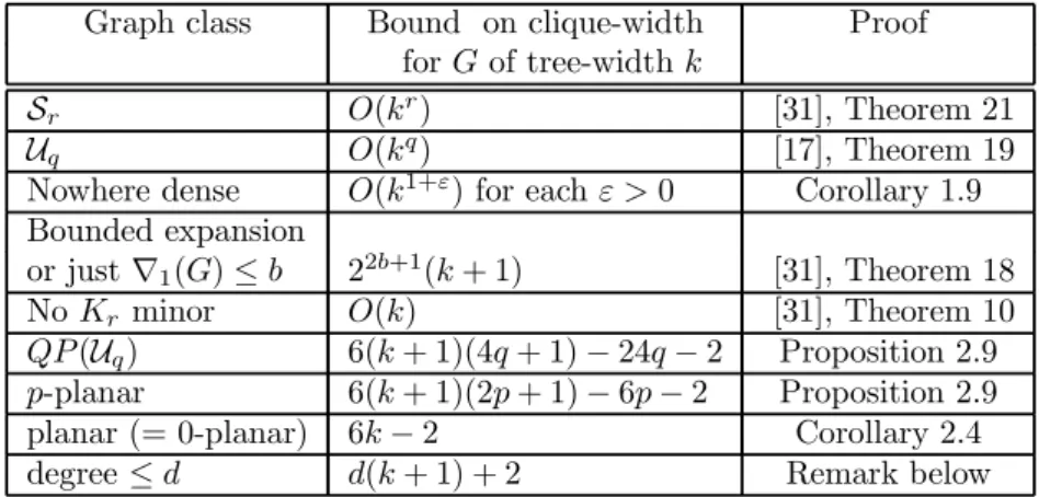
Graph class Bound on clique-width Proof for G of tree-width k
Sr O(kr) [31], Theorem 21
Uq O(kq) [17], Theorem 19
Nowhere dense O(k1+ε) for each ε > 0 Corollary 1.9
Bounded expansion
or just∇1(G)≤ b 22b+1(k + 1) [31], Theorem 18
No Kr minor O(k) [31], Theorem 10
QP (Uq) 6(k + 1)(4q + 1)− 24q − 2 Proposition 2.9
p-planar 6(k + 1)(2p + 1)− 6p − 2 Proposition 2.9 planar (= 0-planar) 6k− 2 Corollary 2.4 degree≤ d d(k + 1) + 2 Remark below
Table 2.
Remark : For a graph G of degree at most d and a set Y of k vertices, each
vertex of Y belongs to at most d sets NG(x)∩Y for x /∈ Y , because it has degree
at most d. Hence, λG(k)≤ kd + 1, and cwd(G) ≤ d(twd(G) + 1) + 2.
3
Descriptions in monadic second-order logic
The main objective is here to prove that 1-planarity is not monadic second-order expressible22 (MS-expressible in short). Under the assumption that P = N P ,
this follows from the fact that 1-planarity is NP-complete for graphs of bounded tree-width [4], because otherwise, it would be decidable in linear-time23 [20, 26].
2 1From (2), one gets cwd(G) ≤ 2λ
G(twd(G) + 1) − 1, to be compared with Theorem 1.8. 2 2Monadic second-order logic is reviewed in the next subection.
2 3Since every MS definable graph property is decidable in linear time on any class of bounded
However, we think interesting to give a proof that does not depend on the P = N P assumption. Furthermore, our construction shows that additional conditions like considering graphs of bounded degree do not make 1-planarity MS-expressible.
We will also consider particular classes of 1-planar graphs that are MS de-finable. A 1-planar graph is optimal if it has the maximum number of edges, that is 4n− 8, for n vertices. It is u-1-planar, which means uniquely 1-planarly
embeddable, if any two 1-planar drawings are homeomorphic, as embeddings in
the sphere. We denote by U1P the class of u-1-planar graphs. An optimal 1-planar graph is u-1-planar unless it is isomorphic to one of particular graphs denoted by XW2k, cf. [48].
We first review a few definitions about monadic second-order logic (only those needed). The reader knowing it (cf. [18, 19, 20, 21]) can skip the next subsection.
3.1
MS formulas and transductions from words to graphs.
Logical expression of graph properties.
For representing a graph G, we use the logical structure VG, edgG where
edgG is the binary symmetric ajacency relation. We identify G and VG, edgG .
Monadic second-order logic (MS logic in short ; see [20] for a thorough study)
allows set quantifications (but no quantifications on relations, such as subrela-tions of edgG). Set variables are capital letters ; they denote sets of vertices.
The following MS sentence24 ϕ :
∃X, Y.(X ∩ Y = ∅ ∧ ∀u, v.{edg(u, v) =⇒
[¬(u ∈ X ∧ v ∈ X) ∧ ¬(u ∈ Y ∧ v ∈ Y )∧
¬(u /∈ X ∪ Y ∧ v /∈ X ∪ Y )]}) expresses that G is 3-colorable (X, Y and VG− (X ∪ Y ) are the three color
classes). Formally, G is 3-colorable if and only if G|= ϕ. Hence, 3-colorability is MS-expressible.
For expressing that G is a cycle with at least 3 vertices, we use : 3vertices∧ degree2 ∧ connectivity.
Connectivity is expressed by : ¬∃X.(X = ∅ ∧ (∃x.x /∈ X)∧
∀u, v.{edg(u, v) =⇒ (u ∈ X =⇒ v ∈ X)}).
The reader will easily write the sentences 3vertices expressing that the graph has at least 3 vertices and degree2 expressing that all its vertices have degree 2.
Edge set quantifications.
We already defined25 Inc(G), the incidence graph of G = V
G, edgG . Here,
we consider it as the bipartite graph VG ∪ EG, incG where EG is the set of
edges and incG is the incidence relation : incG(e, u) holds if and only if u is an
end of edge e.
An edge of G becomes a vertex in Inc(G); it is no longer defined as a pair of vertices. The edges are the elements that occur as first components of pairs in incG. Hence, an MS formula over a structure W, inc intended to be some
Inc(G) can distinguish the edges from the vertices of the potential graph G and check that it is actually an incidence graph. An MS formula over VG∪EG, incG
can use edge set quantifications to express a property of G. An MS2 graph
property is a property that is expressed on incidence graphs by an MS sentence.
An example of an MS2property that is not MS-expressible is the existence of a
Hamiltonian cycle. It is expressed in Inc(G) by :
"there exists a set X ⊆ EG such that the graph Inc(G)[X∪ VG] is
a cycle"
However, for each q, the same properties of graphs inUq are MS2 and
MS-expressible. Formally, every MS sentence ϕ written with inc can be translated into an MS one ϕ[q], written with edg, such that, for every graph G in U
q we
have G|= ϕ[q] if and only if Inc(G)|= ϕ (Chapter 9 of [20]).
Properties of words.
Let A be a finite alphabet. A nonempty word26 w over A of length n is
represented by the logical structure S(w) := [n],≤, (laba)a∈A where each i∈
[n] is a position, i.e., an occurrence of some letter. The binary relation ≤ is the order of positions and the unary relations labaindicate where letters occur
: laba(u) is true if and only if a occurs at position u. Formulas of MS logic
use quantified variables denoting here sets of positions of the considered word represented by S(w).
For an example, the formula
∃X∀u.(u ∈ X =⇒ (laba(u)∨ ∃v.(v /∈ X ∧ u < v ∧ labb(u))))
says that there is a set X of positions that are either occurrences of a, or are before a occurrences of b not in X. Note the use of u < v abreviating u≤ v ∧ ¬(u = v).
2 5in a more concrete way.
2 6A+ denotes the set of nonempty words over A, and A∗ denotes A+ together with the
A well-known result [50] says that a language L⊆ A+is regular if and only
if it is MS definable, which means that there exists an MS sentence ϕ such that w∈ L if and only if S(w) |= ϕ.
Languages of the form L0 := {(ab)ncn | n ≥ 1} or L1 := {(ab)ncm | n ≥
3m+4}, to take two typical examples, are not MS definable because they are not regular. The latter fact is proved as follows. For every language L and word u, L/u :={v ∈ A∗
| uv ∈ L}. If L is regular, there are only finitely many distinct languages L/u. But there are infinitely many languages L0/(ab)nc ={cn−1} for
n≥ 1, and similarly, L1/(ab)nc. Hence, L0and L1are not regular.
Monadic second-order transductions.
Monadic second-order transductions are transformations of logical structures specified by MS formulas. We only review the very particular ones that will be used in the proof of Theorem 3.4. They transform words into graphs.
Let us fix A as above and two MS formulas α and η(x, y) written with ≤ and the unary relation symbols laba(u) (x, y are free first-order variables in η).
Let τ be the partial mapping from words in A+to graphs, defined as follows
: τ(w) = G if and only if
S(w) = V,≤, (laba)a∈A |= α and, if this is true,
G := V, edg where the edge relation edg is defined by: edg(x, y) :⇐⇒ S(w) |= η(x, y).
The positions in w are made into vertices of G. The formula η(x, y) must be written so that the relation it defines is symmetric and irreflexive27 (as τ
defines undirected and loop-free graphs).
The main fact we will use about transductions is the following lemma, a special case of the Backwards Translation Theorem, Theorem 7.10 of [20].
Lemma 3.0 : If τ is an MS transduction and ϕ is an MS sentence, then, the set of words w such that τ (w)|= ϕ is MS definable and is thus a regular language.
Proof sketch: We let ψ be obtained from ϕ by replacing each atomic formula
edg(u, v) by η(u, v). Then, the words w such that τ (w)|= ϕ are those such that S(w)|= α ∧ ψ.
To prove that a graph property P is not MS definable, it suffices to construct τ such that the set of words w such that τ (w) satisfies P is not regular. We will do that for proving Theorem 3.4.
2 7To ensure this, one can take η(x, y) of the form (η′(x, y) ∨ η′(y, x)) ∧ x = y for some MS
3.2
1-planarity is not MS definable
We need some definitions and notation. Definitions 3.1.
(a) Let G be a graph. We denote by P (x1, x2, ..., xn) where n≥ 2, a path from
x1to xn, with vertices x1, x2, ..., xnin this order, and by C(x1, x2, ..., xn) where
n ≥ 3, a cycle with vertices x1, x2, ..., xn, such that we have P (x1, x2, ..., xn)
and an edge x1xn.
Consider a drawing D of G in the plane, with possible edge crossings. A cy-cle C(x1, x2, ..., xn) without any self-crossing (no two of its edges cross) induces
two open regions of the plane: the bounded one is denoted by R(x1, x2, ..., xn)
and the unbounded one by R∞
(x1, x2, ..., xn). The edges, i.e., the curve
seg-ments representing the edges of C(x1, x2, ..., xn), are not in R(x1, x2, ..., xn)∪
R∞(x
1, x2, ..., xn). If the cycle has self-crossings, it determines at least three
open regions of the plane. It separates two vertices u and v if these vertices are (that is, the corresponding points are) in different regions, and then, any path between u and v must cross some edge of the cycle or go through one of x1, x2, ..., xn.
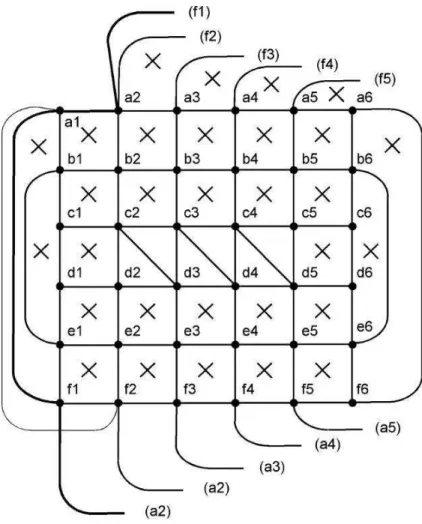
Two drawings are homeomorphic if they are so as embeddings in the sphere. (b) For n ≥ 4, let Gn be the graph with vertices ai, bi, ci, di, ei, fi for i =
1, ..., n. Figure 1 shows G6. A cross in a quandrangular face indicates two edges
that cross, for instance a1b2 and a2b1.
The graph Gn has 6n vertices and 24n− 8 − (n − 3) = 23n − 5 edges.
It is 1-planar but not optimal because of the n− 3 missing edges dici+1 for
i = 2, ..., n− 2. It has 8 vertices of degree 6, 2n − 6 of degree 7 and all others have degree 8.
We let Qn be the planar subgraph induced by the vertices ci and di for
i = 2, ..., n− 1.
Proposition 3.2 : Each graph Gn has a unique 1-planar drawing.
Proof: We will compare the (natural) 1-planar drawing D of Gn (Figure 1
shows D for G6, from which the general case is easily understood) to an
arbi-trary 1-planar drawing D. Without loss of generality (since we consider graph embeddings in the sphere) we can assume that all vertices (except a1, a2, f1) are
in the bounded region R(a1, a2, f1) of D, as in Figure 1 for D. In this figure,
the edges of C(a1, a2, f1) are the thickest ones. Note that a2f1is crossed by the
"thin" edge a1f2; hence the unbounded region R∞(a1, a2, f1) contains half of
the edge a1f2and no vertex. We will prove that D it is homeomorphic to D. In
our discussion, points (vertices), edges, triangles (3-cycles), cycles, regions etc. will refer to D.
First, observe that in any 1-planar drawing, a 4-cycle has at most one cross-ing.
Claim 1 : Let C(x, y, z) be a triangle in Gnand u, v be distinct vertices not
in{x, y, z}. There are at least four edge-disjoint paths between u and v that avoid the vertices x, y, z. The triangle C(x, y, z) does not separate u and v.
Proof : Let H := Gn− {x, y, z}. Removing any 3 edges of H keeps it
con-nected. Hence, by Menger’s Theorem ([25], Section 3.3), there are at least 4 edge-disjoint paths between u and v in H. These paths are in Gn and they
avoid x, y, z. Let us give an example:
u = d1, v = di, x = ci, y = ci+1, z = di+1, 2≤ i ≤ n − 1.
We have the four edge-disjoint paths: P (d1, d2, ..., di), P (d1, e1, e2, ..., ei−1, di),
P (d1, b1, b2, ..., bn, en, en−1, ..., ei+1, di) and
P (d1, c1, b1, a1, a2, ..., an, fn, fn−1, ..., fi, ei, di).
Going back to the general case, if the triangle C(x, y, z) separates u and v, then one of its edges must be crossed twice. This is not possible.
Claim 2 : Let C(x, y, z) = C(a1, a2, f1). Then R(x, y, z) does not contain
any vertex.
Proof: We have R(x, y, z) ⊂ R(a1, a2, f1). Assume a1 ∈ {x, y, z). If u ∈/
R(x, y, z), then C(x, y, z) separates a1 and u which contradicts Claim 1. The
proof is the same with a2 or f instead of a1.
Claim 3 : Let C(x, y, z) be as in Claim 2. If one edge of C(x, y, z), say xy,
is crossed by an edge uv, then u or v is z and the two edges, xz and yz are not crossed.
Proof : By Claim 2, no end of uv is in R(x, y, z). Hence, u or v is z. If
another edge would cross xz, it should have an end equal to y, but it would cross also uz (or vz). This contradicts 1-planarity.
Claim 4 : Let C(x, y, z) and C(x, y, u) be triangles such that{x, y, z, u} ∩
{a1, a2, f1} = ∅. Either R(x, y, z) and R(x, y, u) are disjoint, and we may have
an edge zu crossing xy, or they overlap (i.e., R(x, y, z)− R(x, y, u) = ∅ and R(x, y, u)− R(x, y, z) = ∅), xy is not crossed, and either xz crosses yu or yz crosses xu. If C(x, y, v) is a third triangle such that v /∈ {a1, a2, f1} then xy is
not crossed.
Proof: In a planar drawing, either R(x, y, z) and R(x, y, u) are disjoint, or
one is included in the other, that is, either z∈ R(x, y, u) or u ∈ R(x, y, z). As D is 1-planar, we may have in the first case edge zu crossing xy. We cannot have z∈ R(x, y, u) or u ∈ R(x, y, z) by Claim 2, hence the second case cannot happen. As D is 1-planar, we may also have xz crossing yu or yz crossing xu, but not both. By Claim 3, xy is not crossed.
If we have three triangles sharing the edge xy, two of them overlap. Hence, xy is not crossed.
Claim 5 : Let C(x, y, z) and C(u, v, w) be such that {x, y, z, u, v, w} ∩
{a1, a2, f1} = ∅. If R(x, y, z) and R(u, v, w) overlap, then these two triangles
Proof: By Claim 2, the two triangles share a vertex, say x = u. Assume for
a contradiction that{y, z} ∩ {v, w} = ∅. If xy and xz do not cross vw, then, again by Claim 2, {y, z} ∩ R(u, v, w) = ∅, hence, R(x, y, z) ∩ R(u, v, w) = ∅ contradicting the hypothesis. Assume xy crosses vw, then xz does not (otherwise vw has two crossings) and yz does not cross any edge of C(u, v, w). Hence, either v or w is in R(x, y, z) which contradicts Claim 2. Hence,{y, z}∩{v, w} = ∅ which proves the statement. The two triangles are thus as in Claim 4.
Next we consider D[Qn]. This drawing is a union of triangles that contain
no vertex. We will prove that it is planar. (The graph Qn is planar but this does
not imply that the 1-planar drawing D[Qn] is because c3c4 might cross d3d4.)
We consider a 4-cycle C(ci, di, di+1, ci+1) where 2 ≤ i ≤ n − 2. Its vertices are
denoted for simplicity and respectively by c, d, d′
, c′
. We will also use b denoting bi and d′′denoting di+2.
Claim 6 : The edge cc′
does not cross dd′
and the edge cd does not cross c′
d′
.
Proof: Assume for getting a contradiction that cc′
crosses dd′
, so that cd does not cross c′
d′
.
Consider the triangle C(b, c, c′
). The edge dd′
crosses cc′
, and thus cannot cross edge bc or bc′. Hence, C(b, c, c′) separates d and d′. This is impossible by
Claim 1 as there are 4 edge-disjoint paths between d and d′ that avoid b, c, c′
(one of them can be dd′
).
Assume now similarly that cd crosses c′
d′
, so that cc′
does not cross dd′
.The vertex d′′
will play the role of b in the previous proof. The triangle C(c′
, d′
, d′′
) separates c and d, which contradicts Claim 1.
Hence, the cycle C(c, d, d′
, c′
) is not self-crossing.
Claim 7 : No edge of Qn is crossed by any edge of Gn.
Proof : Each edge of the Hamiltonian cycle C(c2, c3, ..., cn−1, dn−1, ..., d3, d2)
of Qnis incident with three triangles, hence, is not crossed by Claim 4. An edge
crossing cidi+1 should link di and ci+1, and an edge crossing cidi should link
ci−1and di. But the graph Gn has no such edges.
As there are no crossings between edges of Qn, the drawing D[Qn] is planar.
Furthermore, by Claim 2, none of its triangles contains any vertex.
Hence, D[Qn] is as in Figure 1: the drawing is outerplanar with Hamiltonian
(external) cycle C(c2, c3, ..., cn−1, dn−1, ..., d3, d2). All other edges of Qn are in
R(c2, c3, ..., cn−1, dn−1, ..., d3, d2).
We now prove the main statement. We consider a 1-planar drawing D of Gn
and D as in Figure 1. For both of them, all vertices except a1, a2, f1are in the
Let Gn be obtained from Gnby adding the edges dici+1for i = 2, ..., n−2. It
is an optimal 1-planar graph because it has a 1-planar drawing and its number of edges is 23n− 5 + n − 3 = 4 · 6n − 8.
By Claim 7, we can transform D and D into 1-planar drawings of Gn by
putting each additional edge dici+1 inside R(di, di+1, ci+1, ci) that contains
al-ready a single edge and no vertex. We obtain two 1-planar drawings of Gn.
They are homeomorphic because Gn is optimal and is not one of the special
graphs XW2k (cf. [48]). Hence D and D are also homeomorphic, by the same
homeomorphism.
For proving Theorem 3.4, we define, for n≥ 4 and m ≥ 0, the graph Hn,m
as Gn augmented with m new vertices g1, ..., gm and edges forming the path
P (d2, g1, g2, ..., gm, cn−1).
Lemma 3.3 : Hn,mis 1-planar if and only if m≥ 2n − 8. It is u-1-planar
if and only if m = 2n− 8.
Proof: If m≥ 2n − 8, we obtain a 1-planar drawing of Hn,mby putting :
g1 in R(c2, c3, d3), g2in R(c3, d3, d4), g3in R(c3, c4, d4),...,
g2n−9 in R(cn−3, cn−2, dn−2),
and the remaining vertices, g2n−8, ..., gm, in R(cn−2, dn−2, dn−1).
We now prove that, if m < 2n− 8, we cannot do any similar construction. Let us fix n. Assume D is a 1-planar drawing of Hn,m where m < 2n− 8
and m is minimal with this property. It induces a drawing of Gn that must be
homeomorphic to that of Figure 1, by Proposition 3.2.
The path P := P (d2, g1, g2, ..., gm, cn−1) has no self-crossing, otherwise, we
can shorten it and obtain a 1-planar drawing of Hn,m′ where m′< m.
No edge of Gnapart from cidi+1for i = 2, ..., n−2, and cidifor i = 2, ..., n−2,
can be crossed. Hence P must be drawn inside R(c2, c3, ..., cn−1, dn−1, ..., d3, d2).
It must cross 2n− 7 edges, hence have at least 2n − 8 intermediate vertices. We cannot have m < 2n− 8.
If m > 2n− 8, these intermediate vertices can be placed in different ways. If m = 2n− 8, the way described above is the unique one.
We will use the transductions described in Section 3.1.
Theorem 3.4 : The class 1P of 1-planar graphs and the class U1P of uniquely 1-planary embeddable graphs are not monadic second-order definable. Proof: We define Hn,mfrom a word w of the form (abcdef )ngmover the
alphabet A := {a, b, c, d, e, f, g}. Each position in the word w is a vertex of Hn,m. The i-th occurrence of letter a is ai, and similarly for bi, ci, di, ei, fi, gi.
The edges of Hn,mare described by a first-order formula relative to the structure
S(w) = P,≤, (labx)x∈A where P := [6n+m] is the set of positions of w. It says
occurrence of a and the following occurrence of b, between the last occurrence of a and the last occurrence of f , etc.
Hence, Hn,mis the image of S(w) under an MS-transduction τ. This
trans-duction maps the words of the regular language W := {(abcdef)ngm | n ≥
4, m≥ 0} to the graphs Hn,m, in a bijective way.
If 1-planarity would be MS-expressible, then, by Lemma 3.0, the language L := W∩τ−1(1P) would be MS definable, hence regular. But L = {(abcdef)ngm
| n ≥ 4, m ≥ 2n − 8} and this language is not regular (we recalled in Subsection 3.1 how such a fact can be proved). If the classU1P would be MS definable, then the language{(abcdef)ng2n−8| n ≥ 4} would be regular, which is not the
case either, by a similar argument.
It follows that 1-planar graphs are not characerized by finitely many forbid-den configurations such as minors, subgraphs or induced subgraphs. This is not surprizing because 1-planarity is an NP-complete property [12, 22]. They are even not characterized by an infinite set of forbidden induced subgraphs that would be MS definable, as are comparability graphs and interval graphs [15].
A natural question is then : What additional conditions might may 1-planarity MS-expressible ?
Our proof yields a corollary for three classes of graphs. One of them isH, the class of graphs having a Hamiltonian cycle and a 1-planar drawing where any two edges of this cycle do not cross.
Next, we recall that a rotation system for a graph G describes the circular ordering of the edges incident to each vertex u in some drawing in the plane, either planar or not (see [14]). In the logical setting, this circular order is defined as a ternary relation N ext(u, x, y) that means : ux and uy are edges, and uy follows ux in the circular order of edges, according to some fixed orientation of the plane. We have Next(u, x, x) if ux is the unique edge incident with u. Each drawing of the graph (with possible crossings) yields a rotation system, but this drawing may not be reconstructible from the rotation system. A pair (G, N ext) of a graph and a rotation system is called a map (see [14]). A map (G, N ext) is 1-planar if G has a drawing whose associated rotation system is Next.
Corollary 3.5: The following classes of structures are not MS definable: (1) for each d ≥ 8, the class of 1-planar graphs of degree at most d or of path-width at most d,
(2) the classH,
(3) the class of 1-planar maps.
Proof : (1) This is immediate because the graphs Hn,m have maximal
degree 8 and path-width at most 8.
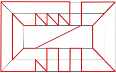
(2) Each graph Hn,m where n is odd (and at least 5) has a Hamiltonian
cycle. If m≥ 2n − 8, then Hn,mhas a 1-planar drawing where such a cycle has
Figure 2: A non-self-crossing Hamiltonian cycle in a graph H7,m (for any m).
be inferred. (The Hamiltonian cycle a1, ..., a5, b5, c5, b4, c4, ..., f1is shown with
bolder edges. We do not show all edges for clarity).
We replace the language W of the proof of Theorem 3.4 by the regular language
W′
:={(abcdef)2p+1gm| p ≥ 2, m ≥ 0}.
IfH would be MS definable, then the language W′
∩ τ−1
(H) = {(abcdef)2p+1gm| p ≥ 2, m ≥ 2(2p + 1) − 8}
would be regular, which is not the case.
(3) Each graph Hn,mcan be equipped with a rotation system Nextn,msuch
that the map Mn,m := (Hn,m, N extn,m) is 1-planar if and only if Hn,m is.
The relation N extn,mis easily described by a first-order formula γ(u, x, y).This
formula will express that Nextn,m(u, x, y) holds if, to take only a few clauses as
examples :
u is an occurrence of letter c, x is the occurrence of c following u and y is the occurrence of letter d that follows x, or,
u is an occurrence of c, y is the occurrence of d following u and x is the occurrence of d that follows y, or,
y, u, x are three consecutive occurrences of letter g.
Hence, we have an MS transduction that construct Mn,mfrom a word. The
proof continues as in the other cases.
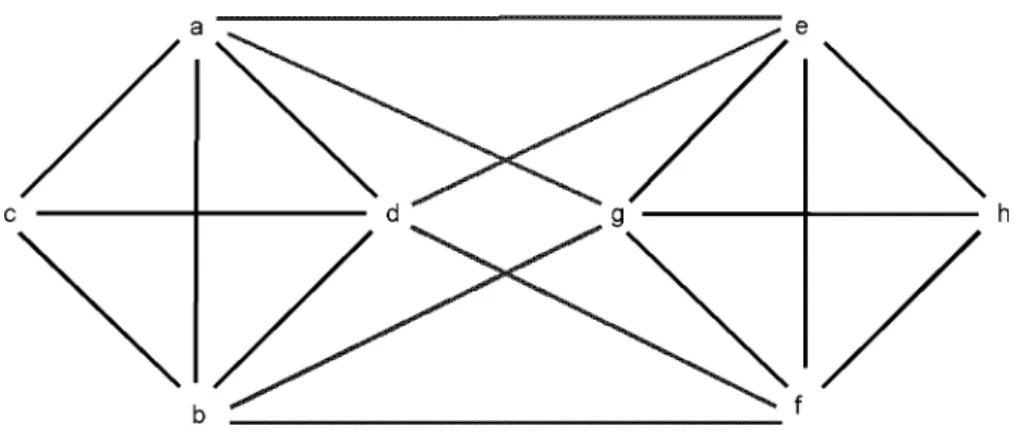
Remark: An alternative construction.
Let us define Jn,m as G4 augmented with new vertices g1, ..., gm, h1, ..., hn,
is 1-planar if and only if n≤ m. The proof of Theorem 3.4 is easily adapted. However, cf. Corollary 3.5, the graphs Jn,m have unbounded degree, and no
Hamiltonian cycle for large n; nevertheless, they have path-width at most 8 and a rotation system for Jn,m, as in the proof of Corollary 3.5 can be defined from
a word (abcdef )4gmhn that defines it.
Edge-set quantifications do not help.
Theorem 3.4 deals with MS sentences that do not use edge-set quantifica-tions. As 1-planar graphs are uniformly 4-sparse, MS2 sentences are no more
powerful than MS ones to express their properties (cf. Section 3.1). Hence, The-orem 3.4 also shows that the classes 1P and U 1P are not MS2 definable.
Some positive monadic second-order expressibility results.
We denote byOpP the class of outer p-planar graphs28, that is, that have
a Hamiltonian cycle and a simple p-planar drawing such that this cycle has no self-crossing and all other edges are inside the bounded region it defines. The classO1P is included in H considered in Corollary 3.5.
An outer 1-planar graph is actually planar : consider a corresponding draw-ing; the edges not in the Hamiltonian cycle C can be put into two sets, say F and F′
each of them having no two crossed edges; then the edges of F′
can be redrawn outside of C, and we get a planar drawing. We prove in the appendix that its tree-width is at most 3.
Proposition 3.6: The class of optimal 1-planar graphs and the class of outer 1-planar graphs are MS definable.
Proof: We will use MS2sentences to define these classes.
Optimal graphs. By Theorem 11 of [48], a graph G is optimal (as 1-planar
graph) if and only if it consists of a 3-connected quandragulated planar graph H and edges added in the following way : for each 4-cycle C(x, y, z, u) of H, one adds the (crossing) edges xz and yu.
An MS2 sentence for describing these graphs can be written of the form
∃F.ϕ(F ) where F is denotes a set of edges and ϕ(F ) expresses the following conditions relative to a graph G :
(a) Every vertex is the end of an edge in F,
(b) the graph H := (VG, F ) is 3-connected and planar, it has no 3-cycle and
every p-cycle for p≥ 5 has a chord,
(c) for every edge xz not in F , there is in H a 4-cycle of the form C(x, y, z, u), (d) for every 4-cycle C(x, y, z, u) of H, the edges xz and yu are in EG− F.
Outer 1-planar graphs. They are described by an MS2 sentence of the form
∃F.ψ(F ) where F denotes a set of edges and ψ(F ) expresses the following con-ditions relative to a graph G :
(a) F is the set of edges of a Hamiltonian cycle C,
2 8Not to be confused with that of p-outer planar graphs that have tree-width at most 3p − 1