HAL Id: hal-00296521
https://hal.archives-ouvertes.fr/hal-00296521
Submitted on 11 Apr 2008
HAL is a multi-disciplinary open access
archive for the deposit and dissemination of
sci-entific research documents, whether they are
pub-lished or not. The documents may come from
teaching and research institutions in France or
abroad, or from public or private research centers.
L’archive ouverte pluridisciplinaire HAL, est
destinée au dépôt et à la diffusion de documents
scientifiques de niveau recherche, publiés ou non,
émanant des établissements d’enseignement et de
recherche français ou étrangers, des laboratoires
publics ou privés.
mid-latitudes: comparisons between MANTRA balloon
measurements and the Canadian Middle Atmosphere
Model
S. M. L. Melo, R. Blatherwick, J. Davies, P. Fogal, J. de Grandpré, J.
Mcconnell, C. T. Mcelroy, C. Mclandress, F. J. Murcray, J. R. Olson, et al.
To cite this version:
S. M. L. Melo, R. Blatherwick, J. Davies, P. Fogal, J. de Grandpré, et al.. Summertime stratospheric
processes at northern mid-latitudes: comparisons between MANTRA balloon measurements and the
Canadian Middle Atmosphere Model. Atmospheric Chemistry and Physics, European Geosciences
Union, 2008, 8 (7), pp.2057-2071. �hal-00296521�
www.atmos-chem-phys.net/8/2057/2008/ © Author(s) 2008. This work is distributed under the Creative Commons Attribution 3.0 License.
Chemistry
and Physics
Summertime stratospheric processes at northern mid-latitudes:
comparisons between MANTRA balloon measurements and the
Canadian Middle Atmosphere Model
S. M. L. Melo1,2, R. Blatherwick7, J. Davies4, P. Fogal2, J. de Grandpr´e5, J. McConnell3, C. T. McElroy4, C. McLandress2, F. J. Murcray7, J. R. Olson7, K. Semeniuk3, T. G. Shepherd2, K. Strong2, D. Tarasick4, and B. J. Williams-Rioux6,1
1Canadian Space Agency, Quebec, Canada
2Department of Physics, University of Toronto, Ontario, Canada
3Department of Earth and Space Science and Engineering, York University, Ontario, Canada 4Environment Canada, Ontario, Canada
5Environment Canada, Quebec, Canada
6Department of Atmospheric and Oceanic Sciences, McGill University, Quebec, Canada 7Department of Physics and Astronomy, University of Denver, Colorado, USA
Received: 2 July 2007 – Published in Atmos. Chem. Phys. Discuss.: 8 August 2007 Revised: 14 February 2008 – Accepted: 10 March 2008 – Published: 11 April 2008
Abstract. In this paper we report on a study conducted us-ing the Middle Atmospheric Nitrogen TRend Assessment (MANTRA) balloon measurements of stratospheric con-stituents and temperature and the Canadian Middle Atmo-sphere Model (CMAM). Three different kinds of data are used to assess the inter-consistency of the combined dataset: single profiles of long-lived species from MANTRA 1998, sparse climatologies from the ozonesonde measurements during the four MANTRA campaigns and from HALOE satellite measurements, and the CMAM climatology. In doing so, we evaluate the ability of the model to repro-duce the measured fields and to thereby test our ability to describe mid-latitude summertime stratospheric processes. The MANTRA campaigns were conducted at Vanscoy, Saskatchewan, Canada (52◦N, 107◦W) in late August and early September of 1998, 2000, 2002 and 2004. During late summer at mid-latitudes, the stratosphere is close to photo-chemical control, providing an ideal scenario for the study reported here. From this analysis we find that: (1) reducing the value for the vertical diffusion coefficient in CMAM to a more physically reasonable value results in the model bet-ter reproducing the measured profiles of long-lived species; (2) the existence of compact correlations among the con-stituents, as expected from independent measurements in the literature and from models, confirms the self-consistency of
Correspondence to: S. M. L. Melo
(stella.melo@space.gc.ca)
the MANTRA measurements; and (3) the 1998 measure-ments show structures in the chemical species profiles that can be associated with transport, adding to the growing ev-idence that the summertime stratosphere can be much more disturbed than anticipated. The mechanisms responsible for such disturbances need to be understood in order to assess the representativeness of the measurements and to isolate long-term trends.
1 Introduction
The science of stratospheric ozone gained a new dimension when it became clear that ozone depletion, and ultimately its anticipated recovery, is linked to climate change in a com-plex way. Temperature, humidity, winds, and the presence of other chemicals in the atmosphere influence ozone forma-tion and transport, and the presence of ozone, in turn, af-fects those atmospheric fields through radiative processes. Although the existence of such a link now seems intuitive, a detailed description of the processes and their relative im-portance remains a challenge. Understanding the processes that control the ozone budget and the proper representation of such processes in atmospheric models are recognized in recent assessments as fundamental to projecting ozone re-covery and to further explore the effects of ozone on climate and vice versa (WMO, 2007; IPCC/TEAP, 2005).
In contrast to the large ozone loss observed in the Antarctic spring (up to 70%) and in the Arctic during cold winters (up to 30%), ozone depletion at mid-latitudes has been shown to be much smaller (3% to 6% since the 1970s) (WMO, 2007). It is also less understood and more difficult to model. As first pointed out by Dobson, the ozone total column mea-sured at different mid-latitude locations will differ depend-ing on the synoptic meteorological conditions (Dobson et al., 1926). Therefore, small trends are difficult to detect and de-mand statistical analysis of long-term data sets. Similarly, the attribution of any such small trend is challenging.
Different mechanisms have been proposed to explain the observed mid-latitude ozone trends involving chemical (Solomon et al., 1998) and dynamical (Hadjinicolaou et al., 1997; Hood et al., 1997; Appenzeller et al., 2000, Hadjini-colaou et al., 2002) processes. So far, most of the work in the field focuses on a single mechanism, although it is cur-rently accepted that a combination of mechanisms is needed to explain the observations (see for example Chiperfield and Jones, 1999; Millard et al, 2003; Durry and Hauchecorne, 2005; Berthet et al., 2006; WMO, 2007; and references therein).
While chemical processes are local, dynamical processes normally involve links between mid and high latitudes. Pro-cesses such as changes in circulation and the transport of ozone-depleted air from polar latitudes have been proposed to explain the mid-latitude ozone deficit. However, the rela-tive importance of each process remains unclear.
Statistical analysis using zonally averaged total ozone data indicates that the observed summertime ozone trend over the northern hemisphere mid-latitudes can be entirely ex-plained by the springtime trends there, as the photochemi-cally damped remnant of the mid-latitude springtime trends (Fioletov and Shepherd, 2003). The importance of such re-sults, as emphasized by the authors, is that it implies no need to invoke anomalous summertime ozone chemistry to explain summertime ozone trends. While the same rela-tion between springtime and summertime mid-latitude trends does not hold in the southern hemisphere, Fioletov and Shep-herd (2005) showed that the relation holds in both hemi-spheres when applied to the entire extra-tropics, but fails for southern mid-latitudes because of the contribution of springtime polar losses to summertime mid-latitude ozone trends, via transport. The extent of this contribution, esti-mated statistically, is consistent with that from detailed mod-elling studies. In the northern hemisphere, the contribu-tion of polar ozone loss to midlatitude summertime trends is within the uncertainty level of the statistical analysis. How-ever, model simulations (Chipperfield and Jones, 1999; Mil-lard et al., 2003) and measurements conducted in brief cam-paigns (Ross et al., 2004; Durry and Hauchecorne, 2005) support the hypothesis of vortex air contributing to the mid-latitude ozone deficit detected at summertime in the north-ern hemisphere. Recently, Ross et al. (2004) and Durry and Hauchecorne (2005) reported on the presence of long-lived
remnants of the wintertime polar vortex in the mid-latitude summer stratosphere in June 2000.
In addition to the trends, transient decreases in column ozone levels over single stations at mid-latitudes have been observed during summertime and reported in several com-munications (Orsolini and Nikulin, 2006; Kar et al., 2002, and references therein). Those events have been referred to as low-ozone episodes, and although they have been as-sociated with a conjunction of a deep tropospheric anticy-clone and the displacement above the anticyanticy-clone of the mid-stratospheric pool of low-ozone (Orsolini and Nikulin, 2006), the mechanism remains a subject of debate.
It is clear that the required level of understanding of the processes governing the mid-latitude ozone balance cannot be achieved by models or observations alone, but rather through a combination of both. Such a synthesis not only aids in the interpretation of the observations, but also helps identify model deficiencies and thereby leads to the improve-ment of the representation of physical processes in the mod-els, and hence in their predictive capabilities.
In this paper we report on co-located measurements of ozone, temperature, and long-lived species made dur-ing four Middle Atmospheric Nitrogen TRend Assessment (MANTRA) balloon campaigns conducted in different years and compare them with results from the Canadian Middle Atmosphere Model (CMAM), a coupled chemistry-climate model. We use three different kinds of data to assess the inter-consistency of the combined dataset: single profiles of long-lived species from MANTRA 1998, sparse clima-tologies from the ozonesonde measurements during the four MANTRA campaigns and from HALOE satellite measure-ments, and the CMAM climatology. Our objectives are: (1) to test the ability of CMAM to reproduce summertime mid-latitude conditions, (2) to investigate the validity of corre-lations among long-lived species as predicted by the model, and (3) to use CMAM as a support to interpret the MANTRA measurements.
The use of a chemistry-climate model, like CMAM, for studies involving comparisons with measurements has the advantage of allowing us to test our understanding of physi-cal processes. MANTRA provides an ideal scenario for such a study since the experiments were conducted in late summer, at “turnaround”, when the stratospheric zonal wind changes from easterly to westerly. During the summertime easterly period, planetary wave activity is minimal and the strato-sphere is dynamically quiescent (e.g., Wunch et al., 2005), while photochemistry is dominant. Therefore, at turnaround, the stratosphere is close to photochemical control (Fahey et al., 2000; Fioletov and Shepherd, 2003).
2 Measurements
MANTRA is a set of balloon campaigns aimed at inves-tigating the changing chemical balance of the Northern
Hemisphere mid-latitude stratosphere, with a particular fo-cus on the nitrogen budget and its role in the depletion of mid-latitude ozone. A review of the MANTRA campaigns is provided by Strong et al. (2005). We provide here only a brief description of the campaigns and the instruments used to acquire the data used in this paper.
MANTRA campaigns were conducted at Vanscoy, Saskatchewan (52◦N, 107◦W) during the period when the stratospheric zonal wind velocity changes its sign. Turnaround of the stratospheric winds occurs twice each year at mid-latitudes: in the early spring and in late summer (see Wunch et al., 2005 for more details). Under such conditions, the stratospheric winds are at a minimum, ensuring that the payload remains within the telemetry range (approximately 400 km) for the duration of the mission (typically 18 h). Four campaigns were conducted, with large-balloon launch dates of 24 August 1998, 29 August 2000, 3 September 2002, and 1 September 2004. Ozonesondes were also launched with varying frequency during each campaign.
The vertical profiles of temperature and ozone partial pres-sure discussed here were meapres-sured by the ozonesondes dur-ing all four campaigns, while the N2O, CH4, HNO3, and HCl mixing ratio profiles were measured by the Denver Univer-sity Fourier Transform Spectrometer (DU-FTS) during the 1998 campaign. We preserve in this analysis the units in which the measurements were provided.
2.1 Denver University Fourier Transform Spectrometer (DU-FTS)
This instrument, as well as the technique employed for the retrieval of each species, is fully described in Fogal et al. (2005) and is only briefly described here. It has a strong heritage since it has taken part in other balloon campaigns and has been used extensively as a ground-based instrument at many locations, including Fairbanks, Alaska and the South Pole (for example see Murcray et al., 1980). DU-FTS is a BOMEM DA2 Michelson type interferometer-spectrometer with 50 cm input optics. The optical path difference is 50 cm, resulting in an unapodized full-width half-maximum res-olution of approximately 0.01 cm−1. The measurements ex-tend from 700–1300 cm−1in one channel (with the mercury-cadmium-telluride detector) and from 2650–3250 cm−1 in the other channel (indium antimonide detector). The scan time was about 80 s. A biaxial solar tracking telescope was used to maintain the input solar beam on the interferometer window. During the 1998 MANTRA balloon flight, spectra were acquired during the sunset occultation.
The measured spectra were analyzed by fitting synthetic spectra generated with the Denver University line-by-line, layer-by-layer computer code RADCO (RADiation COde) (Blatherwick et al., 1989) to the observed spectra. Mixing ratio profiles were generated from the sunset spectra using the “onion peeling” technique. The pressure and temperature profiles used as input to RADCO were based on radiosonde
data for the day of the flight, and the line parameters were taken from HITRAN96 (Rothman et al., 1998). Measure-ment uncertainties (error bars shown in the plots) were esti-mated from uncertainties in the RADCO inputs (the pressure, temperature profile and the line parameters) and in the sensi-tivity of the quality of fit to variations in the retrieved mixing ratio (i.e., the mixing ratio in the tangent layer).
2.2 The ozonesondes
During all four MANTRA campaigns, ozone profiles were obtained on a nearly daily basis by electrochemical con-centration cell (ECC) ozonesondes attached to a stan-dard balloon-borne meteorological radiosonde (Komhyr, 1969). Ozone partial pressure is measured from the reaction of ozone with potassium iodide in an aqueous solution. The sondes were prepared and the data analyzed according to the standards used in the Canadian ozonesonde network, which differ only slightly from current WMO recommendations (Tarasick et al., 2005). In addition to the ozone sensor, each instrument package included a standard Vaisala RS-80 ra-diosonde so that pressure, temperature and humidity profiles could be recorded. The precision of these temperature mea-surements is 0.1 K with a pressure-dependent accuracy of 0.2 K from the ground to 50 hPa, 0.3 K between 50 hPa to 15 hPa, and 0.4 K below 15 hPa (Luers, 1997). The ozonesondes measure in situ ozone concentration with a vertical resolution of the order of 100 m. Estimation of errors for ozonesonde measurements from inter-comparison campaigns and labora-tory tests indicate that in the troposphere (below about 12 km altitude), the precision of the ECC-sonde is better than ±(5– 10)% with a small positive bias of about 3%. From 12 to 25 km altitude the precision is found to be better than ±(5%). Above 27 km factors such as loss of air pump efficiency, in-strument temperature changes, slow secondary reactions and sensing solution evaporation render the sonde measurements less reliable (WCRP, 1998; Smit et al., 2007; Deshler et al., 2008; Davies et al., 2000).
3 The Canadian Middle Atmosphere Model (CMAM) The CMAM is an upward extension of the Canadian Cen-tre for Climate Modelling and Analysis General Circulation Model (CCCma GCM) up to 0.0006 hPa (roughly 100 km al-titude) (Beagley et al., 1997). The model incorporates middle atmosphere radiation, interactive chemistry and gravity-wave drag, as well as all the processes in the GCM. For the version used in this work (referred to as version 7) prognostic vari-ables are computed in spectral space using T32 horizontal resolution (corresponding to just under 6◦latitude and lon-gitude) and 65 vertical levels (about 2 km resolution in the middle atmosphere but higher resolution below 25 km).
CMAM includes a comprehensive representation of strato-spheric chemistry (de Grandpr´e et al., 1997) with 31
Days of Measurements
0
1
2
3
4
0 9 -A u g 1 0 -A u g 1 1 -A u g 1 2 -A u g 1 3 -A u g 1 4 -A u g 1 5 -A u g 1 6 -A u g 1 7 -A u g 1 8 -A u g 1 9 -A u g 2 0 -A u g 2 1 -A u g 2 2 -A u g 2 3 -A u g 2 4 -A u g 2 5 -A u g 2 6 -A u g 2 7 -A u g 2 8 -A u g 2 9 -A u g 3 0 -A u g 3 1 -A u g 0 1 -S e p 0 2 -S e p 0 3 -S e p 0 4 -S e p 0 5 -S e p 0 6 -S e p 0 7 -S e p 0 8 -S e p 0 9 -S e p 1 0 -S e p 1 1 -S e p 1 2 -S e p1998
2000
2002
2004
Total
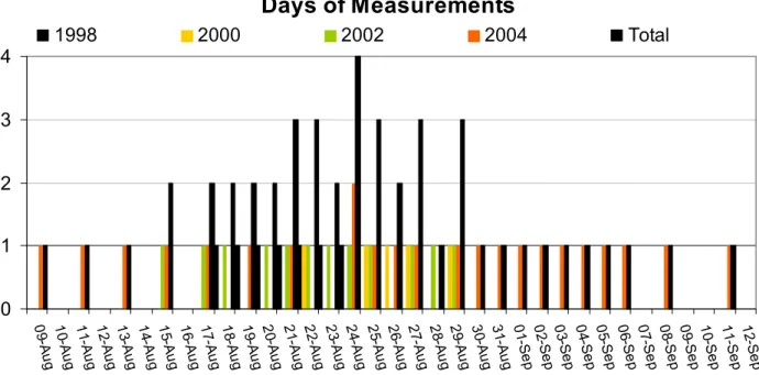
Fig. 1. Days on which the ozonesondes were launched, for each campaign year. Also shown is the sum of the number of ozonesondes profiles
for each day, considering all four campaigns.
non-advected species and 16 advected species and fami-lies. Concentrations of the long-lived source gases are im-posed in the troposphere. Transport of species is accom-plished using spectral advection. Heterogeneous reactions of ClNO3, N2O5and BrNO3take place on sulphate aerosols. In the polar regions, heterogeneous reactions occur on strato-spheric ternary solution, and water-ice; no sedimentation or nitric acid trihydrate particle formation on polar stratospheric clouds is included. Details about how the chemical species are calculated can be found in de Grandpr´e et al. (1997). A slightly more recent version of CMAM (differing only in its dynamical aspects, which are not of great importance in the late summer midlatitude stratosphere) has been recently as-sessed in the model intercomparison of Eyring et al. (2006); more detailed comparisons of CMAM ozone with observa-tions can be found in Tegtmeier and Shepherd (2007), Heg-glin and Shepherd (2007), and Shepherd (2008).
The CMAM data used here comprise years 28–48 from a timeslice simulation representing conditions in the year 2000. Profiles are generated for the model grid point closest to Vanscoy, and at various solar zenith angles. For this run CMAM was sampled in approximately 10 min increments, producing 144 profiles per day. In these simulations, clima-tological sea-surface temperatures are imposed and, although varying from month to month, are kept constant from year to year. Also, phenomena like the quasi-biennial oscillation and solar and aerosol variability, which are known to be signifi-cant factors affecting the inter-annual variability of the strato-sphere, are not included in the model version used here. As
a consequence, the inter-annual variability in the model as reported here could be underestimated. However, a study by Wunch et al. (2005), using both the National Centers for Environmental Prediction/National Center for Atmospheric Research (NCEP/NCAR) reanalysis and the United King-dom Meteorological Office (MetO) analysis products, sug-gests that the CMAM appears to have a realistic level of dy-namical variability for the time and location of the MANTRA measurements. This dynamical variability in CMAM is as-sociated with Rossby normal modes, whose behaviour varies from year to year, and induces variability in ozone and long-lived chemical species (Pendlebury et al., 2008).
4 Results
4.1 Ozone and temperature
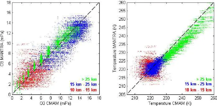
During the four MANTRA campaigns, a large number of ozone profiles were collected allowing calculation of average profiles that can be used for comparisons with CMAM. The measurements extend from 9 August to 11 September, being concentrated around 24 August, for which the largest num-ber of profiles is available (four). Seven ozonesondes were launched in 1998, five in 2000, 12 in 2002, and 23 in 2004, making a total of 47 ozone and temperature profiles available for this analysis. Figure 1 shows a distribution of the mea-surements as a function of day of year for all the campaigns. Measurements and model fields are compared qualita-tively in Fig. 2, in scatter plots using all the ozonesonde
Fig. 2. Scatter plots for ozone and temperature, comparing MANTRA measurements with CMAM data for all four campaigns. CMAM data
are daily averages (see text). The different colors correspond to ozone and temperature values in different altitude ranges: red for altitudes between 10 and 15 km, blue for altitudes between 15 and 25 km, and green for altitudes above 25 km.
measurements and the matching model days. Different al-titude ranges are shown in different colours. In order to rec-oncile differences in altitude resolution between the model (∼1.3 km) and the measurements (∼0.2 km), the ozonesonde data are smoothed to the CMAM resolution. Nevertheless the finite vertical resolution of the CMAM is apparent in the banded structure of the ozone scatter plots above 25 km, where the vertical gradient of ozone partial pressure is large and the model resolution somewhat coarser than below 25 km. A model day is calculated as the average of the 144 model profiles produced daily for ozone and temperature, for each year of the model run. Thus, for each measurement point there are at least 19 corresponding model points (one for each model year). The dotted line represents the 1:1 cor-relation. From Fig. 2 we see that the points are generally distributed around the 1:1 correlation line, indicating overall consistency between model and measurements. Scatter about the 1:1 correlation line is expected because of day-to-day dy-namical variability in both model and measurements, since CMAM is a free-running model without reference to any spe-cific year. The temperature plot in Fig. 2 shows that points corresponding to altitudes above 25 km, that is, in the upper stratosphere, tend to be consistently located below the 1:1 correlation line suggesting the model overestimates the tem-peratures in this altitude range. This suggested warm bias in CMAM is consistent with the warm bias in the global-mean temperature which indicates a radiative bias in the model in the upper stratosphere (Pawson et al. 2000, Eyring et al., 2006). A caveat of our analysis is that the measurements
span over a period of eight years (made every other year) and may not well represent climatology.
MANTRA measurements are further compared to the CMAM statistically. In this analysis we used model daily av-eraged ozone profiles from 9 August to 11 September. Since the observation period spans about a month, we fitted a lin-ear trend to the model data for each altitude to account for the seasonal cycle, so as to be able to include all the data in the comparison. Examples of the magnitude of the linear trend are shown in Fig. 3 where ozone and temperature at two given altitudes (15 and 24 km, chosen arbitrarily) are plotted as a function of day of year (from 9 August to 11 September), with each curve corresponding to a different model year. As this figure illustrates, the linear trend becomes important for both ozone and the temperature only above 15 km altitude. After removing the linear trend, the ozone and temperature daily averaged profiles from the 19 years of the model sim-ulation are combined in an ensemble to build the CMAM mean and determine the CMAM standard deviation.
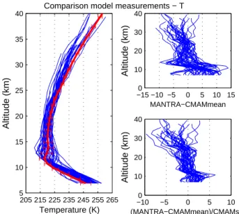
MANTRA ozonesonde measurements are smoothed and interpolated to the CMAM altitude grid. Then the CMAM linear trend, for each altitude, is subtracted from the MANTRA measurements in order to remove the effect of the seasonal cycle. Note that such a trend cannot be es-timated from the measurements themselves because there are not sufficient measurements to define the seasonal cy-cle. The MANTRA ozone and temperature profiles (after removing the linear trend) are shown in Figs. 4 and 5, to-gether with the CMAM mean profiles. The error bars in the
0 5 10 15 20 25 30 35 1 3 5 7 9 11 13 15 17 O3 (partial pressure) 0 5 10 15 20 25 30 35 210 215 220 225 230 235
Days (from 9 August to 11 September)
Temperature (K)
Fig. 3. CMAM Ozone and temperature as a function of the days
(from 9 August to 11 September) for each year of the model run at 24 km (green curves) and 15 km (red curves) altitudes. The black line represents the fitted linear trend.
0 2 4 6 8 10 12 14 16 18 5 10 15 20 25 30 35 40
Ozone (partial pressure)
Altitude (km)
Comparison model and measurements − O
3 −5 −2.5 0 2.5 5 7.5 0 10 20 30 40 MANTRA−CMAMmean Altitude (km) −100 0 10 20 10 20 30 40 (MANTRA−CMAMmean)/CMAMstd Altitude (km)
Fig. 4. MANTRA ozone measurements compared with the CMAM
as: (a) all the MANTRA ozone profiles (blue) after removing the CMAM linear trend together with the CMAM mean profile (red). The error bars in the CMAM mean profile represent the CMAM standard deviation; (b) MANTRA ozone profiles (after removing the CMAM linear trend) minus the CMAM mean; and (c) same as (b) divided by the CMAM standard deviation.
CMAM mean profiles represent the standard deviation (1σ ). Also shown in the same figures are the ozone and temper-ature anomalies (MANTRA-CMAM mean) and the anoma-lies divided by the CMAM standard deviation ((MANTRA-CMAM mean)/((MANTRA-CMAM std). The largest absolute variability in ozone is found below about 15 km where mixing of strato-spheric and tropostrato-spheric air is expected, and at the ozone peak region (between 20 and 25 km). By looking at each year individually we found that the large variability in the
205 215 225 235 245 255 265 5 10 15 20 25 30 35 40 Temperature (K) Altitude (km)
Comparison model measurements − T
−15 −10 −50 0 5 10 15 10 20 30 40 MANTRA−CMAMmean Altitude (km) −100 −5 0 5 10 10 20 30 40 (MANTRA−CMAMmean)/CMAMstd Altitude (km)
Fig. 5. Same as Fig. 4, for temperature.
MANTRA measurements at the peak region is dominated by the 1998 measurements, while for altitudes below 15 km it is a common feature for all the 4 years. Again there is a clear suggestion of a warm bias in the model above about 25 km. One important point to keep in mind is the lower reliability of ozonesonde measurements above about 27 km due to instru-mental factors such as loss of air pump efficiency, instrument temperature changes, slow secondary reactions and sensing solution evaporation (WCRP, 1998).
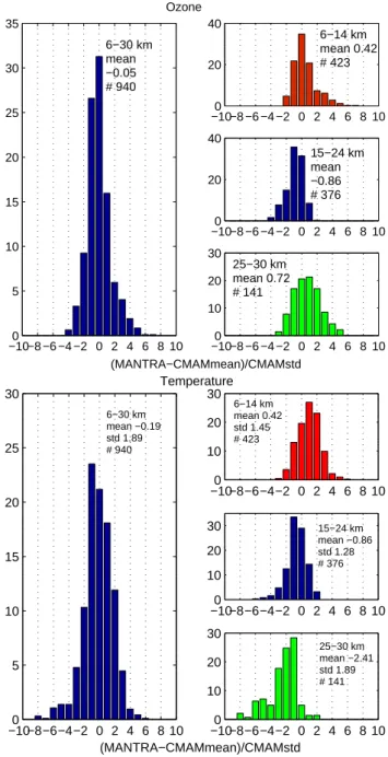
The ensemble of all ozone and temperature measurements, normalized as above ((MANTRA-CMAM mean)/CMAM std), is shown in Fig. 6 as histograms. The histograms are shown as frequency of occurrence (number of occurrence di-vided by the total number of points) per bin of 1 CMAM standard deviation. If the measurements and model agreed perfectly, these histograms would have a mean of zero and a standard deviation of unity. On the left side of Fig. 6 the his-tograms are constructed using the full altitude range, and on the right side for different altitude ranges. For this analysis we limited the altitude at 30 km given the decreasing relia-bility of the ozonesonde data above about 27 km altitude (as discussed above).
The ozone histogram from 6–14 km shows a distinct skew-ness, with a long tail corresponding to high ozone fluctua-tions. This makes physical sense, as the vertical gradient of ozone is much larger above the tropopause than it is below, so there is an asymmetry between the distribution of high and low fluctuations. A similar but slightly less pronounced skewness is seen in the CMAM ozone histograms (not shown), reflecting the underestimated tropopause variability that would be expected of a relatively low-resolution model such as CMAM. Indeed, from the 6–14 km temperature histogram in Fig. 6, temperature fluctuations in this altitude range seem underestimated by CMAM; in units of CMAM
std, the observed temperature std is 1.45.
In the altitude range 15–24 km, both the ozone and tem-perature histograms have standard deviations close to unity, indicating that the model variability is quite realistic in this altitude range. Once again, the largest difference between model and measurement temperatures occurs for altitudes above about 25 km, with the model mean temperature lying 2.41 σ above the measurements.
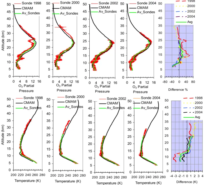
The model and measurement profiles are further compared as averages for individual years in Fig. 7. For this compari-son the measurements are averaged for each campaign year and compared to the model averaged profile (constructed as before). Furthermore, the average profiles of the mea-surements for each year are further averaged to build what we call the averaged sonde profiles in Fig. 7, referred to as “Av Sondes” in the figure and as measurement climatology in this text. The model ozone and temperature fields are first daily averaged, as discussed above, and further averaged for the period of 9 August to 11 September to encompass the pe-riod for which the measurements are available. Then, the 19 resulting averaged model profiles, one for each model year, are averaged again, building what we refer to as CMAM in Fig. 7. Ozone is shown as partial pressure since this is the standard ozonesonde product. Differences between the mea-surement and model (in percent for ozone and in Kelvin for temperature) as a function of altitude are quantified in the right panel in Fig. 7. While this comparison does not take in account the seasonal cycle (as done in Figs. 4, 5 and 6), it allows us to focus on the behaviour of individual MANTRA years. The largest differences are seen for the measurements made in 1998, indicating the atmosphere was more disturbed during 1998 than during the other years.
One interesting feature in Fig. 7 is the measurement of a significant depletion of about 40% of ozone at the peak al-titude during the 1998 MANTRA campaign. While such a feature would not be unusual in individual profiles, its persis-tence throughout the 1998 campaign is striking. This feature is further discussed in the next section.
As seen in Figs. 2, 5, and 6 the largest differences in the temperature profiles are seen above about 25 km, reaching 2 K in single-year average profiles. Note that the precision of the Vaisala sensors is expected to be within 0.3 K. Although this error may increase for higher altitudes in response to the slowing in rotation of the sensor, increasing its sensitivity to the orientation with respect to the sun, it is not expected to exceed 1 K (Luers, 1997). Also, as noted above, this sug-gested warm bias in CMAM is consistent with the warm bias in the global-mean temperature which indicates a radiative bias in the model (Pawson et al., 2000; Eyring et al., 2006).
The shallow layer of enhanced static stability observed in Fig. 7 just above the tropopause, seen in both the sondes and the model, is the tropopause inversion layer described by Birner et al. (2006), which is stronger in summer and a ubiquitous feature in CMAM (albeit somewhat too high and somewhat too deep).
−10−8 −6 −4 −2 0 2 4 6 8 100 5 10 15 20 25 30 35 Ozone −10−8 −6 −4 −2 0 2 4 6 8 100 20 40 (MANTRA−CMAMmean)/CMAMstd −10−8 −6 −4 −2 0 2 4 6 8 100 20 40 −10−8 −6 −4 −2 0 2 4 6 8 100 10 20 30 6−30 km mean −0.05 # 940 15−24 km mean −0.86 # 376 6−14 km mean 0.42 # 423 25−30 km mean 0.72 # 141 −10−8−6−4−2 0 2 4 6 8 100 5 10 15 20 25 30 Temperature −10−8−6−4−2 0 2 4 6 8 100 10 20 30 (MANTRA−CMAMmean)/CMAMstd −10−8−6−4−2 0 2 4 6 8 100 10 20 30 −10−8−6−4−2 0 2 4 6 8 100 10 20 30 6−30 km mean −0.19 std 1.89 # 940 15−24 km mean −0.86 std 1.28 # 376 6−14 km mean 0.42 std 1.45 # 423 25−30 km mean −2.41 std 1.89 # 141
Fig. 6. Histogram of the differences between the measurements and
the model mean (divided by the model standard deviation) for ozone (upper panels) and temperature (lower panels). The larger plots, on the left, show the histograms for the altitude range from 6 to 30 km. The right side small plots compare the model and measurements in different altitude regions: 14≥z≥6 km upper, 24≥z≥15 km middle left, and 30≥z≥25 km lower corner. The points are grouped and counted for occurrence in bins of 1 model standard deviation.
0 5 10 15 20 25 30 35 40 45 50 0 4 8 12 16 O3 Partial Pressure Al ti tu d e ( k m ) Sonde 1998 CMAM Av_Sondes 0 5 10 15 20 25 30 35 40 45 50 0 4 8 12 16 O3 Partial Pressure Sonde 2000 CMAM Av_Sondes 0 5 10 15 20 25 30 35 40 45 50 -80 -40 0 40 80 Difference % 1998 2000 2002 2004 Avg 0 5 10 15 20 25 30 35 40 45 50 0 4 8 12 16 O3Partial Pressure Sonde 2002 CMAM Av_Sondes 0 5 10 15 20 25 30 35 40 45 50 0 4 8 12 16 O3Partial Pressure Sonde 2004 CMAM Av_Sondes 0 5 10 15 20 25 30 35 40 45 50 200 220 240 260 280 Temperature (K) A lt it u d e (k m ) Sonde 1998 CMAM Av_Sondes 0 5 10 15 20 25 30 35 40 45 50 200 220 240 260 280 Temperature (K) Sonde 2000 CMAM Av_Sondes 0 5 10 15 20 25 30 35 40 45 50 200 220 240 260 280 Temperature (K) Sonde 2002 CMAM Av_Sondes 0 5 10 15 20 25 30 35 40 45 50 200 220 240 260 280 Temperature (K) Sonde 2004 CMAM Av_Sondes 0 5 10 15 20 25 30 35 40 45 50 -4 -3 -2 -1 0 1 2 3 4 Difference (K) 1998 2000 2002 2004 Avg
Fig. 7. Ozone (upper panels) and temperature (bottom panels) sonde measurements during the four MANTRA campaigns. Also shown
is CMAM climatology for August-September covering the measurement period (see text). The differences between each yearly averaged profile (measurement) to the model average for all campaigns (CMAM), for ozone (in percent: ((CMAM-MANTRA)*100/MANTRA) and for temperature (in Kelvin: CMAM-MANTRA), are shown on the right-hand panels, respectively.
4.2 Long-lived species
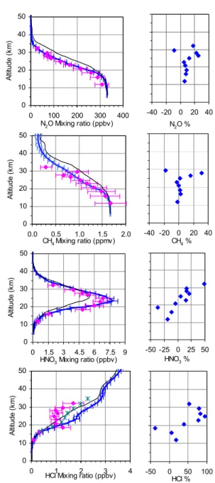
During the 1998 campaign, the balloon-borne DU-FTS mea-sured simultaneous vertical profiles of N2O, CH4, HNO3, and HCl during a single sunset. We compare here these four measured profiles with CMAM fields as shown in Fig. 8. As done before for ozone and temperature, the CMAM fields shown here represent a 20 year average for the period of 11 August to 11 September. The mean CMAM profile of each species is calculated using all the daily mean profiles over the period of 11 August to 11 September, for all the model years. The error bars are the standard deviation (1σ ).
The differences between measurement and model (curves labelled CMAM V7) are quantified in percent ([CMAM-MANTRA]/MANTRA) as a function of altitude for each species and shown in the right panels of Fig. 8. Note that the tropospheric value of N2O in CMAM was inadvertently set about 4% too high, so all CMAM nitrogen fields can be expected to also be 4% too high. When that difference is ac-counted for the CMAM N2O profile agrees very well with the MANTRA observations.
It is instructive to compare this version of CMAM with a previous version (referred to as CMAM V5 in Fig. 8) which had a much higher value of the vertical diffusivity (and
slightly reduced vertical resolution), namely Kzz=1.0 m2s−1 rather than the current Kzz=0.1 m2s−1. The smaller value is more realistic (being consistent with the upper bound in-ferred from aircraft measurements of trace species), and im-proves other model features, as discussed below, whereas the larger value is so strong as to play a first-order role in vertical transport, especially in summer when the Brewer-Dobson downwelling is so weak (Shepherd, 2007). The re-sults shown in Fig. 8 suggest that such a change does indeed have a first-order effect on the tracer profiles, and that once the vertical diffusion is reduced to a sufficiently small value, the model agrees well with the measurements. Note that the diffusion coefficient and the slightly reduced vertical resolu-tion are the sole changes between CMAM V5 and CMAM V7 that might have first-order effects on the constituent pro-files.
From Fig. 8 we observe that the N2O mixing ratio is repro-duced by the model within 10% up to about 25 km altitude, above which the difference increases, reaching 25%. If we account for the 4% high bias in the tropospheric N2O, this difference reduces accordingly and falls within the measure-ment error bars, suggesting the model reproduces the mea-surements within the measurement error bars even for the higher altitudes. The model CH4agrees with the measure-ments within 7% up to about 25 km, above which the mea-surements show an increase in mixing ratio followed by a sharp decrease higher up, leading to differences larger than 30% between model and measurements above 30 km. Such structure in the CH4mixing ratio climatological profile is not expected, and is most probably related to layers of different air mass origin.
Because the measurements are single profiles, they are prone to sampling variability. Although the late summer is dynamically quiescent compared with the fall, winter and spring, as noted earlier, there is growing evidence that dy-namically induced variability would still be present. For ex-ample, in a recent analysis Pendlebury et al. (2008) suggested the importance of day-to-day variability in the stratosphere associated with the 5-, 10- and 16-day Rossby normal modes which will induce variability in temperature and chemical fields. Their analysis shows that all three modes have max-imum amplitudes near 50◦N and that they could and likely would exist during the MANTRA campaign in late August and early September.
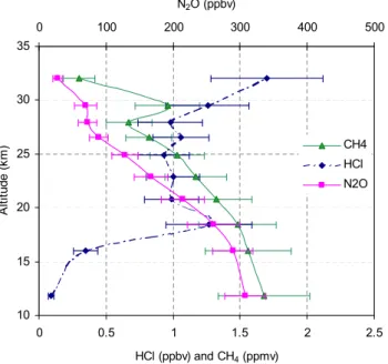
The CH4 and N2O measurements are directly compared in Fig. 9. As discussed in Fogal et al. (2005) the struc-ture observed above about 25 km in the CH4 profile is co-located in altitude with a somehow less pronounced structure in the N2O profile. Structures in N2O and CH4profiles oc-curring between 23 to 30 km at mid-latitude have been re-cently reported by Huret et al. (2006) as being present in the SPIRALE (Spectrom`etre Infra Rouge pour l’ ´Etude de l’Atmosph`ere par Diodes Laser Embarqu´ees) measurements conducted at Aire sur l’Adour launch base (France, 43.7◦N, 0.3◦W) on 2 October 2002. Given its high vertical resolution
-40 -20 0 20 40 N2O % 0 10 20 30 40 50 0 100 200 300 400 N2O Mixing ratio (ppbv) A lti tu d e ( k m ) 0 10 20 30 40 50 0.0 0.5 1.0 1.5 2.0 CH4Mixing ratio (ppmv) A lti tu d e ( k m) -40 -20 0 20 40 CH4 % 0 10 20 30 40 50 0 1.5 3 4.5 6 7.5 9 HNO3 Mixing ratio (ppbv)
A lti tu d e ( k m) -50 -25 0 25 50 HNO3 % 0 10 20 30 40 50 0 1 2 3 4 HCl Mixing ratio (ppbv) A lti tu d e ( k m) -50 0 50 100 HCl %
Fig. 8. The left panels show the vertical profiles of N2O, CH4,
HNO3and HCl measured with the DU-FTS during sunset as part
of the MANTRA 1998 campaign (pink curves). The blue dia-monds represents CMAM V7 climatology over Vanscoy, Saska-toon. The error bar in the model output represents the model vari-ability (see text). The black lines represent the CMAM V5 cli-matology also for Vanscoy, August. The green symbols in the HCl plot represent HALOE climatological values for August at MANTRA coordinates. The right panels show the differences in percent (100%*(CMAM V7-MANTRA)/MANTRA) for each con-stituent.
(of the order of 5 meters) the SPIRALE measurements show that N2O and CH4 profiles can in fact be highly disturbed with layers of structures that can be associated to different mixing processes taking place in the atmosphere.
10 15 20 25 30 35 0 0.5 1 1.5 2 2.5 HCl (ppbv) and CH4 (ppmv) Al ti tu d e ( k m ) 0 100 200 300 400 500 N2O (ppbv) CH4 HCl N2O
Fig. 9. Vertical profiles of N2O, CH4and HCl measured with the
DU-FTS during the sunset part of the MANTRA 1998 campaign.
The altitude resolution of the MANTRA measurements would not allow us to clearly separate layers of mixing as is done with the SPIRALE measurements. Nevertheless, both sets of measurements show that the mid-latitude stratosphere can be more active dynamically than normally expected.
The HNO3model and measurement profiles (Fig. 8) show differences of the order of 10% at the peak altitude (about 24 km) increasing to about 20% for higher altitudes and to about 25% below the peak. Differences of about 50% are seen for altitudes above 30 km. HNO3is the main constituent of the NOy family below about 25 km. Although the dif-ferences between model and measurements could suggest problems in the model NOy partitioning, those differences are within the measurement errors estimation. Therefore, we conclude that the model reproduces the measurements of HNO3within the measurement error bars below about 30 km. It is evident from the first three panels of Fig. 8 that chang-ing the vertical diffusivity in the model has brought the model significantly closer to the measurements. HCl is the excep-tion, with the model reproducing the measurements very well at lower altitudes but overestimating the measurements by a factor of two for altitudes above about 20 km. However, as discussed below, the MANTRA HCl profile is rather anoma-lous compared with the other available measurements.
As MANTRA provides only one profile of HCl, it is in-structive to look at other available datasets. The HALOE dataset is the largest dataset available and the only one that covers the period when the balloon measurement was made. Moreover, it has been extensively used in many other anal-yses. The HALOE climatology used here consists of a monthly mean HALOE data set constructed by harmonic
re-10 15 20 25 30 35 40 0.0 0.5 1.0 1.5 2.0 2.5 3.0 3.5 HCl (ppbv) A lt it u d e ( k m )
Fig. 10. Vertical profiles of HCl measured with the DU-FTS
dur-ing the MANTRA 1998 campaign (magenta points), the HALOE (version 19) HCl individual profiles for 28 August 1998 for lati-tudes covering from 45◦N to 46.6◦N and different longitudes (thin dark blue lines), HALOE (version 18) 6-year climatology for Au-gust (thick green line), and the CMAM mean profile (thick black line).
gression of HALOE (version 18 retrieval) profile data repre-sentative of the entire HALOE record (repeating seasonal cy-cles were fit through a 6+ year record). It has been calculated for the period December 1992–February 1997 (prior to De-cember 1992, the large quantities of Mount Pinatubo aerosol in the lower stratosphere gave rise to very large HALOE re-trieval errors). Details of how the HALOE climatologies are constructed can be found at: http://www.sp.ph.ic.ac.uk/ haloe/userguide/uguide.html.
As can be seen in Fig. 8, both MANTRA and model HCl profiles agree well with HALOE for altitudes below about 22 km. However, the MANTRA HCl values are signifi-cantly lower than HALOE climatology for altitudes above 22 km. To further explore this comparison, HALOE individ-ual profiles (version 19 retrieval) are now available from the HALOE data portal at: http://haloedata.larc.nasa.gov/home/ index.php. The closest in latitude and time from MANTRA measurements are HALOE profiles measured on 28 Au-gust 1998 at latitude range of 45◦N to 46.6◦N. We show then in Fig. 10 all the individual HALOE HCl profiles for 28 Au-gust at the latitude range of 45◦N to 46.6◦N corresponding to different longitudes. The presence of structures in HCl profiles above about 20 km is evident from the HALOE data. However, the structures are not as pronounced as observed in the MANTRA HCl measurement.
Compared to HALOE climatology (Fig. 8), CMAM over-estimates HCl above 20 km by about 40%. Comparison of CH4 (not shown here) from HALOE with both MANTRA and CMAM shows differences smaller than 10% throughout
the altitude range for which MANTRA data is available. Re-cent measurements of HCl and CH4made by the ACE-FTS instrument on the Canadian satellite SCISAT were compared to HALOE measurements by McHugh et al. (2005) show-ing that ACE-FTS HCl values are consistently higher than HALOE by 10–20% from 20–40 km altitude and CH4values 10% higher than HALOE throughout. These results suggest then that the CMAM reproduces ACE-FTS measurements, giving confidence in the model.
The DU-FTS is an instrument with a strong flight heritage that has taken part in several balloon campaigns (Fogal et al., 2005). Although during the MANTRA campaign in 1998 the DU-FTS operated below its optimal performance (which is reflected in the rather larger measurement error bars shown here), a detailed error budget analysis for the instrument by Fogal et al. (2005) leads the authors to conclude that the fea-tures measured above about 23 km in the CH4 and in the N2O are most likely from geophysical rather than instrumen-tal origin. It is also our understanding that measurement and retrieval errors alone could not explain the discrepancies re-ported here between the MANTRA and the model for the HCl profiles. Therefore, we conclude that MANTRA sam-pled an air mass depleted in HCl between about 23 and 30 km altitude and that although the magnitude of such depletion in the MANTRA measurements may be affected by instru-mental errors, the structure in itself is likely of geophysical origin. Given the rather coarse vertical resolution (compared to measurements made with instruments like SPIRALE) and the fact that MANTRA measurements of long-lived species are single profiles, we can not advance this analysis towards the identification of mechanisms causing the structures ob-served in the measurements.
4.3 Compact correlations
One further means of comparing model and measurements and to assess self-consistency in the measurements is through correlations among long-lived species. Correlation plots be-tween long-lived species have been used in the literature as a way of eliminating, in large part, dynamical effects by as-suming different long-lived species are advected in a similar manner. Indeed the existence of a compact correlation be-tween long-lived species has been supported both theoreti-cally (see for example Avallone and Prather, 1997 and refer-ences therein) and experimentally (see for example Loewen-stein et al., 1993; Michelsen et al., 1998).
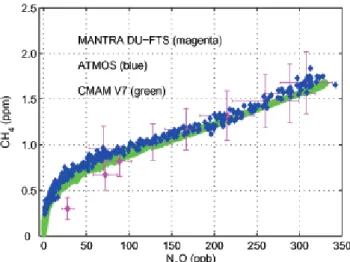
Recently Sankey and Shepherd (2003) used CMAM to in-vestigate the general conditions under which compact cor-relations can be expected to form. One important result of this analysis was to show that a correlation between long-lived species can be characterized even from measurements with limited sampling. Therefore, we use correlation plots to assess the internal consistency of the MANTRA measure-ments. Furthermore, MANTRA measurements can be com-pared with other datasets through correlations. We use the
Fig. 11. Correlation between CH4and N2O mixing ratios as
mea-sured during the MANTRA campaign of 1998 compared with AT-MOS measurements for mid-latitudes and CMAM.
ATMOS measurements for mid-latitudes given the availabil-ity of data for the species of interest.
Figure 11 shows the CH4:N2O correlation plot using MANTRA and ATMOS measurements and CMAM data (all daily averaged values for the period of August 11 to September 11 are shown in plot). Below 25 km (i.e., where CH4>1 ppm), the MANTRA measurements indeed show a linear correlation in agreement with ATMOS measure-ments and with CMAM. As shown before in Sankey and Shepherd (2003), the linear correlation obtained from AT-MOS measurements is well reproduced by CMAM. Al-though Sankey and Shepherd (2003) analysed the version of CMAM with the higher vertical diffusivity, a linear correla-tion should not be affected by the change in vertical diffusiv-ity.
The argument for the existence of a compact correlation between long-lived chemical species is based on the fact that meteorological fluctuations will move air parcels around co-herently, meaning that any correlation that exists between two long-lived species will persist despite the fluctuations. As explained in Sankey and Shepherd (2003), although a ver-tical section of measurements, like the measurements shown here, and a horizontal section (like aircraft measurements, for example) would sample different parts of a single corre-lation, the results will be consistent (see Fig. 1b from Sankey and Shepherd, 2003). For very long-lived chemical species the slope of the correlation curve is independent of alti-tude and the correlation is linear. For intermediate lifetimes (longer than several weeks but shorter than the several-year timescale of the diabatic circulation) the correlation is non-linear. Therefore, although the existence of the correlation is a result of dynamics, the slope of the correlation will depend on chemistry.
The existence of a CH4:N2O compact correlation in the MANTRA measurements below about 25 km with a charac-teristic of mid-latitudes gives us confidence on the measure-ment technique employed during the MANTRA campaign.
As discussed before, from Fig. 9, the CH4 and the N2O profiles are non-monotonic above about 25 km. Indeed, simi-larly as for the SPIRALE measurements discussed in the pre-vious section (Huret et al., 2006), N2O and CH4correlations at this altitude range differ from the mid-latitude correlation values deduced from ATMOS space shuttle measurements by Michelsen et al. (1998). In fact, the MANTRA CH4:N2O correlation above 25 km altitude resembles the ATMOS high latitude correlation in Michelsen et al. (1998). Given the rather coarse vertical resolution of the MANTRA measure-ments together with the fact that we have single profiles of each species, we can not determine the origin of the air mass sampled during the MANTRA measurements. However, the measurements clearly indicate the importance of transport in the upper stratosphere even during the late summer time.
5 Discussion and Summary
The comparison between MANTRA measurements and the CMAM shown here, made for late summer when the mid-latitude stratosphere is comparatively quiescent and nor-mally assumed to be close to photochemical control, suggests that vertical profiles of long-lived species in the model are much improved when the vertical diffusivity is reduced from 1.0 m2s−1to 0.1 m2s−1. As discussed by Shepherd (2007), the lower value is more realistic (being consistent with the upper bound inferred from aircraft measurements of trace species) and sufficiently small to have a negligible impact on mean tracer distributions. On the other hand, the higher value of 1.0 m2s−1is sufficiently large to have a significant effect on the mean tracer distributions. Indeed, Tegtmeier and Shepherd (2007) found that the summertime persistence of ozone anomalies, which is quite realistic in CMAM with a vertical diffusivity of 0.1 m2s−1, is rapidly lost for a diffu-sivity of 1.0 m2s−1. The consistency between the model and the measurements of the long-lived species is reflected in the existence of the compact correlation among measured con-stituents, in agreement with the model prediction and with the literature.
The statistical comparison of the MANTRA measure-ments of ozone and temperature with the CMAM confirm the model capability to reproduce mid-latitude conditions. How-ever, the results indicate a warm bias in the CMAM temper-ature for altitudes above about 25 km. In summary, we con-clude that CMAM has achieved a level of development in which it can reproduce reasonably well not only ozone mea-surements but a suite of atmospheric constituents and tem-perature, such as those reported here.
Our results show also interesting features in the measure-ments taken in 1998. The ozone profiles show a narrow layer
of enhanced ozone at about 12 km. This lower-altitude en-hanced ozone layer is also seen in the average 2000 cam-paign profile but is not evident in 2002 or 2004. However, looking at individual profiles we see that the occurrence of layers of enhanced ozone at altitudes below 15 km is rather common, with their frequency of occurrence and persistence changing from year to year. Similar features have been ob-served in ozone profile data at mid-latitude sites in Europe and Asia (Lemoine, 2004; Hwang et al., 2007). Climato-logically, these layers of enhanced ozone appear to coincide with the temperature ”tropopause inversion layer” discussed by Birner et al. (2006) and shown to be stronger in summer. Although CMAM clearly reproduces this feature in temper-ature (albeit too high and too deep), it is much weaker in ozone.
While the occurrence of filament structures in the ozone profile for altitudes below about 25 km seems to be rather common at mid-latitudes in the winter and spring, and as-sociated with dynamics (Tarasick et al., 2005), the origin of persistent layers of depleted ozone above 20 km in the late summer, as observed in the 1998 dataset used here, seems to be less clear. Kar et al. (2002) conducted a statistical analysis of the frequency of occurrence of layered structures in the vertical profiles of ozone as retrieved by the Strato-spheric Aerosol and Gas Experiment (SAGE II) version 6.0 measurements. Their results show a bimodal peak in the oc-currence of such layers with two maxima: one between 12 and 15 km and another between 22 and 28 km. Their analysis suggests a maximum probability of occurrence of structures in the ozone profile above 20 km altitude for latitudes above 45◦N during summer time. However, a caveat in their anal-ysis is that it makes no distinction between occurrences of enhancement or depletion layers. No identification is made as for the source of those structures in ozone although the authors suggest the structures observed above 20 km altitude could be consistent with remnant air from the polar vortex “frozen-in” into the mean summertime easterly flow as pro-posed by Hess and Holton (1985), and Orsolini (2001), and supported by the analysis by Fairlie et al. (1999). Recently Durry and Hauchecorne (2005) presented evidence for long-lived polar vortex air in the mid-latitude summer stratosphere from in situ laser diode CH4and H2O measurements at Gap, in southern France (44◦N, 6◦E), during June 2000. Indeed, the photochemical lifetime of ozone at altitudes from 20 to 28 km is of the order of 100 days or more.
The observed layer of depleted ozone at around 25 km al-titude during the 1998 is observed in 7 profiles spanning 7 days. However, a similarly persistent feature is not observed in other years. This result suggests that if mixing of air from the polar vortex can generate layers of depleted ozone above 20 km altitude that can persist throughout the summer, im-pacting the estimation of the mid-latitude ozone trend, its importance varies from year to year.
Although the layer of depleted ozone reported here seems consistent with the hypothesis of long lived “fossil” debris
from the polar vortex that can persist till late summer, as modelled by Orsolini (2001), a more in-depth analysis using a chemical transport model would be necessary to confirm it. Nevertheless, it is clear that the origin and persistence of such features need to be better understood as they are likely to affect total column measurements and ultimately to impact our ability to detect ozone trends.
The MANTRA campaign in 1998 measured nonmono-tonic CH4 and N2O profiles above about 25 km altitude. These structures do not seem to be directly related with the O3depleted layer discussed above, suggesting they may re-sult from different mixing processes. The MANTRA HCl profile shows a pronounced depletion between 20 to 30 km altitude. Although less pronounced, similar structures are also present in the HALOE (v19) HCl profiles measured dur-ing late August 1998 at mid-latitudes. The dataset analyzed here does not support a clear identification of the mecha-nisms responsible for the observed structures in the atmo-spheric constituent profiles nor does it define whether they are directly related or resulting from different mechanisms. However, the results discussed have the importance of adding to the growing evidence that the summertime stratosphere is rather dynamically disturbed, although at a lower level than during other seasons. The understanding of those variabil-ities is of particular importance for trend analysis as likely they impact total column measurements and make it diffi-cult to assess bias and reconcile profile measurement of con-stituents made at different years with different instruments.
The results of the analysis presented here show that mod-els like CMAM can provide valuable a priori means and vari-ances useful for the analysis of measurements even though a model might underestimate the variability. It is clear that when a discrepancy is found one needs to look carefully at both model and measurements. However, the model variabil-ity provides a very useful first guess at sampling variabilvariabil-ity, allowing the screening of features in the measurements to separate them into climatologically reasonable or spurious.
Acknowledgements. All MANTRA campaigns have been
sup-ported by the Canadian Space Agency and Environment Canada. MANTRA 1998 also received funding from the Centre for Re-search in Earth and Space Technology, while MANTRA 2002 and 2004 received additional support from the Natural Sciences and Engineering Research Council. The participation of the University of Denver was supported in part by the National Science Foundation and in part by the National Aeronautics and Space Administration. We thank Scientific Instrumentation Limited for payload and launch support, and all team members who contributed to the success of the MANTRA campaigns. The CMAM is funded by the Canadian Foundation for Climate and Atmospheric Sciences, the Canadian Space Agency, and the Natural Sciences and Engineering Research Council. The authors thank the two reviewers and the editor.
Edited by: A. Richter
References
Appenzeller, C., Weiss, A. K., and Stachclin, J.: North Atlantic Oscillation modulates total ozone trends, Geophys. Res. Lett., 27, 1131–1134, 2000.
Avallone, L. M. and Prather, M. J.: Tracer-tracer correlations: Three-dimensional model simulations and comparisons to obser-vations, J. Geophys. Res., 102(D15), 19 233–19 246, 1997. Beagley, S. R., de Grandpr´e, J., Koshyk, J. N., McFarlane, N. A.,
and Shepherd, T. G.: Radiative-dynamical climatology of the first-generation Canadian Middle Atmosphere Model, Atmos.-Ocean., 35, 293–331, 1997.
Berthet, G., Huret, N., Lef`evre, L., Moreau, G., Robert, C., Chartier, M., Catoire, V., Barretz, B., Pisso, I., and Pomathiod, L.: On the ability of chemical transport models to simulate the vertical structure of the N2O, NO2and HNO3species in the mid-latitude
stratosphere, Atmos. Chem. Phys., 6, 1599–1609, 2006, http://www.atmos-chem-phys.net/6/1599/2006/.
Birner, T., Sankey, D., and Shepherd, T. G.: The tropopause in-version layer in models and analyses, Geophys. Res. Lett., 33, L14804, doi:10.1029/2006GL026549, 2006.
Blatherwick, R. D., Murcray, D. G., Murcray, F. H., Murcray, F. J., Goldman, A., Vanasse, G. A., Massie, S. T., and Cicerone, R. J.: Infrared emission measurements of morning N2O5, J. Geophys.
Res., 94, 18 337–18 340, 1989.
Chipperfield, M. P. and Jones, R. L.: Relative influence of atmo-spheric chemistry and transport on arctic ozone trends, Nature, 400, 551–554, 1999.
Davies, J., Tarasick, D., McElroy, C. T., Kerr, J. B., Fogal, P. F. and Savastiouk, V.: Evaluation of ECC Ozonesonde Prepara-tion Methods from Laboratory Tests and Field Comparisons us-ing MANTRA, Proc. Quadrennial Ozone Symposium, Sapporo, Japan, 2000.
de Grandpr´e, J., Sandilands, J. W., McConnell, J. C., Beagley, S. R., Croteau, P. C., and Danilin, M. Y.: Canadian middle atmosphere model: preliminary results from the chemical transport module, Atmos.-Ocean, 35(4), 385–431, 1997.
Deshler, T., Mercer, J. L., Smit, H. G. J., Stubi, R., Levrat, G., Johnson, B. J., Oltmans, S. J., Kivi, R., Thompson, A. M., Witte, J., Davies, J., Schmidlin, F. J., Brothers, G., and Sasaki, T.: Atmospheric comparison of electrochemical cell ozonesondes from different manufacturers, and with different cathode solution strengths: The balloon experiment on standards for ozonesondes (BESOS)., J. Geophys. Res., 113, D04308, doi:10.1029/2007JD008975, 2008.
Dobson, G. M. B., Harrison, D. N., and Lawrence, J.: Measure-ments of the amount of ozone in the Earth’s atmosphere and its relation to other geophysical conditions, Proc. R. Soc. London, Ser. A, 110, 660–693, 1926.
Durry, G. and Hauchecorne, A.: Evidence for long-lived polar vor-tex air in the mid-latitude summer stratophere from in situ laser diode CH4 and H2O measurements, Atmos. Chem. Phys., 5, 1467–1472, 2005,
http://www.atmos-chem-phys.net/5/1467/2005/.
Eyring, V., Butchart, N., Waugh, D. W., Akiyoshi, H., Austin, J., Bekki, S., Bodeker, G. E. B., B. A., Brhl, C., Chipperfield, M. P., Cordero, E., Dameris, M., Deushi, M., Fioletov, V. E., Frith, S. M., Garcia, R. R., Gettelman, A., Giorgetta, M. A., Grewe, V., Jourdain, L., Kinnison, D. E., Mancini, E., Manzini, E., Marchand, M., Marsh, D. R., Nagashima, T., Newman, P. A.,
Nielsen, J. E., Pawson, S., Pitari, G., Plummer, D. A., Rozanov, E., Schraner, M., Shepherd, T. G., Shibata, K., Stolarski, R. S., Struthers, H., Tian, W., and Yoshiki, M.: Assessment of cou-pled chemistry-climate models: Evaluation of dynamics, trans-port characteristics and ozone, J. Geophys. Res., 111, D22308, doi:10.1029/2006JD007327, 2006.
Fahey, D. W., Gao, R. S., Del Negro, L. A., Keim, E. R., Kawa, S. R., Salawitch, R. J., Wennberg, P. O., Hanisco, T. F., Lanzendorf, E. J., Perkins, K. K., Lloyd, S. A., Swartz, W. H., Proffitt, M. H., Margitan, J. J., Wilson, J. C., Stimpfle, R. M., Cohen, R. C., McElroy, C. T., Webster, C. R., Loewenstein, M., Elkins, J. W., and Bui, T. P.: Ozone destruction and production rates between spring and autumn in the Arctic stratosphere, G. Res. Lett., 27, 2605–2608, 2000.
Fairlie, T. D., Pierce, R. B., Al-Saadi, J. A., Grose, W. L., Rus-sell III, J. M., Profitt, M. H., and Webster, C. R.: The contribu-tion of mixing in Lagrangian photochemical prediccontribu-tions of polar ozone loss over the Arctic in summer 1997, J. Geophys. Res., 104, 26 597–26 609, 1999.
Fioletov, V. E. and Shepherd, T. G.: Seasonal persistence of mid-latitude total ozone anomalies, Geophys. Res. Lett., 30, 1417, doi:10.1029/2002GL016739, 2003.
Fioletov, V. E. and Shepherd, T. G.: Summertime total ozone vari-ations over middle and polar latitudes, Geophys. Res. Lett., 32, L04807, doi:10.1029/2004GL022080, 2005.
Fogal, P. F., Blatherwick, R. D., Murcray, F. J., and Olson, J. R.: Infra-red FTS Measurements of CH4, N2O, O3, HNO3, HCl,
CFC-11 and CFC-12 from the MANTRA Balloon Campaign, Atmos.-Ocean, 43(4), 351–359, 2005.
Hadjinicolaou, P., Pyle, A., Chipperfield, P. M., and Kettleborough, J. A.: Effect of interannual meteorological variability on mid-latitude O3, Geophys. Res. Lett., 24, 2993–2996, 1997.
Hadjinicolaou, P., Pyle, J. A., Jrrar, A., and Bishop, L.: The dynam-ically driven long-term trend in stratospheric ozone over northern middle latitudes, Q. J. R. Meteorol. Soc., 128(S83), 1393–1412, 2002
Hegglin, M. and Shepherd, T. G.: O3–N2O correlations from ACE: Revisiting a diagnostic of transport and chem-istry in the stratosphere. J. Geophys. Res., 112, D19301, doi:10.1029/2006JD008281, 2007.
Hess, P. G. and Holton, J. R.: The origin of temporal variance in long-lived trace constituents in the summer stratosphere, J. At-mos. Sci, 42, 1455–1463, 1985.
Hood, L. L., McCormack, J. P., and Labitzke, K.: An investigation of dynamical contributions to midlatitude ozone trends in winter, J. Geophys. Res., 102, 13 079–13 093, 1997.
Huret, N., Pirre, M., Hauchecorne, A., Robert, C., and Catoire, V.: On the vertical structure of the stratosphere at midlatitudes dur-ing the first stage of the polar vortex formation and in the polar region in the presence of a large mesospheric descent, J. Geo-phys. Res., 111, D06111, doi:10.1029/2005JD006102, 2006. Hwang, S.-H., Kim, J., and Cho, G.-R.: Observation of secondary
ozone peaks near the tropopause over the Korean peninsula asso-ciated with stratosphere-troposphere exchange, J. Geophys. Res., 112, D16305, doi:10.1029/2006JD007978, 2007.
IPCC/TEAP Special Report on Safeguarding the Ozone Layer and the Global Climate System: Issues Related to Hydrofluorocar-bons and PerfluorocarHydrofluorocar-bons, 2005.
Kar, J., Trepe, C. R., Thomason, L. W., and Zawodny, J. M.:
Obser-vations of layers of ozone vertical profiles from SAGEII (v6.0) measurements, Geophys. Res. Lett., 29(10), 1443–1446, 2002. Komhyr, W. D.: Electrochemical concentration cells for gas
analy-sis, Ann. Geophys., 25, 203–210, 1969, http://www.ann-geophys.net/25/203/1969/.
Lemoine, R.: Secondary maxima in ozone profiles, Atmos. Chem. Phys., 4, 1085–1096, 2004,
http://www.atmos-chem-phys.net/4/1085/2004/.
Loewenstein, M., Podolske, J. R., Fahey, D. W., Woodbridge, E. L., P. Tin, A. W., Newman, P. A., Strahan, S. E., Kawa, S. R., Schoeberl, M. R. and Lait, L. R.: New observations of the NOy/N2O correlation in the lower stratosphere, Geophys. Res. Lett., 20(22), 2531–2534, 1993.
Luers, J.: Temperature Error of the Vaisala RS90 Radiosonde, J. Atmos. Ocean. Technol., 14(6), 1520–1532, 1997.
Michelsen, H. A., Manney, G. L., and Gunson, M. R.: Correla-tions of stratospheric abundances of NOy, O3, N2O, and CH4
de-rived from ATMOS measurements, J. Geophys. Res, 103(D21), 28 347–28 359, 1998.
Millard, G. A., Lee, A. M., and Pyle, J. A.: A model study of the connection between polar and midlatitude ozone loss in the Northern Hemisphere lower stratosphere, J. Geophys. Res., 108(D5), 8323, 2003.
McHugh, M., Magill, B., Walker, K. A., Boone, C. D., and Bernath, P. F.: Comparison of atmospheric retrievals from ACE and HALOE, Geophys. Res. Lett., 32, L15S10, doi;10.1029/2005GL022403, 2005.
Murcray, F. J., Goldman, A., Murcray, D. G., Cook, G. R., van-Allen, J. W., and Blatherwick, R. D.: Identification of isolated NO lines in balloonborne infrared solar spectra., Geophys. Res. Lett., 7, 673–676, 1980.
Orsolini, Y.: Long-lived tracer patterns in the summer polar strato-sphere, Geophys. Res. Letter, 28, 3855–3858, 2001.
Orsolini, Y. and Nikulin, G.: A low-ozone episode during the Eu-ropean heatwave of August 2003, Q. J. R. Meteorol. Soc., 132, 667–680, 2006.
Pawson, S., Kodera, K., Hamilton, K., Shepherd, T. G., Beagley, S. R., Boville, B. A., Farrara, J. D., Fairlie, T. D. A., Kitoh, A., La-hoz, W. A., Langematz, U., Manzini, E., Rind, D. H., Scaife, A. A., Shibata, K., Simon, P., Swinbank, R., Takacs, L., Wilson, R. J., Al-Saadi, J. A., Amodei, M., Chiba, M., Coy, L., deGrandpr, J., Eckman, R. S., Fiorino, M., Grose, W. L., Koide, H., Koshyk, J. N., Li, D., Lerner, J., Mahlman, J. D., McFarlane, N. A., Me-choso, C. R., Molod, A., O’Neill, A., Pierce, R. B., Randel, W. J., Rood, R. B., and Wu, F.: The GCM-Reality Intercomparison Project for SPARC (GRIPS): Scientific issues and initial results, Bull. Am. Meteorol. Soc., 81, 781–796, 2000.
Pendlebury, D., Shepherd, T. G., Pritchard, M., and McLandress, C.: Normal mode Rossby waves and their effects on chemi-cal composition in the late summer stratosphere, Atmos. Chem. Phys., 8, 1925–1935, 2008,
http://www.atmos-chem-phys.net/8/1925/2008/.
Ross, D. E. M., Pyle, J. A., Harris, N. R. P., McIntyre, J. D., Millard, G. A., Robinson, A. D., and Busen, R.: Investigation of Arc-tic ozone depletion sampled over midlatitudes during the Egrett Campaign of spring/summer 2000, Atmos. Chem. Phys., 4, 141– 168, 2004,
http://www.atmos-chem-phys.net/4/141/2004/.
Ed-wards, D. P., Flaud, J.-M., Perrin, A., Camy-Peyret, C., Dana, V., Mandin, J.-Y., Chroeder, J., McCann, A., Gamache, R. R., Wattson, R. B., Yoshino, K., Chance, K. V., Jucks, W., Brown, L. R., Nemtchinov, V., and Varanasi, P.: The HITRAN molecu-lar spectroscopic database and HAWKS (HITRAN Atmospheric Workstation): 1996 edition, J. Quant. Spectrosc. Radiat. Trans-fer, 60, 665–710, 1998.
Sankey, D. and Shepherd, T. G.: Correlation of long-lived chemi-cal species in a middle atmosphere general circulation model, J. Geophys. Res, 108, 4494, doi:10.1029/2002JD002799, 2003. Shepherd, T. G.: Transport in the middle atmosphere, J. Meteorol.
Soc. Japan, 85B, 165–191, 2007.
Shepherd, T. G., Dynamics, stratospheric ozone, and climate change. Atmos.-Ocean, 46, 371–329, 2008.
Smit, H. G. J., Straeter, W., Johnson, B., Oltmans, S., Davies, J., Tarasick, D. W., Hoegger, B., Stubi, R., Schmidlin, F., Northam, T., Thompson, A., Witte, J., Boyd I., and Posny, F.: Assessment of the performance of ECC-ozonesondes under quasi-flight con-ditions in the environmental simulation chamber: Insights from the J¨ulich Ozone Sonde Intercomparison Experiment (JOSIE), J. Geophys. Res., 112, D19306, doi:10.1029/2006JD007308, 2007. Solomon, S., Portmann, R. W., Garcia, R. R., Randel, W., Wu, F., Nagatani, R., Gleason, J., Thomason, L. W., Poole, L. R. and McCormick, M. P.: Ozone depletion at midlatitudes: coupling of volcanic aerosols and temperature variability to anthropogenic chlorine., Geophys. Res. Letter, 25, 1871–1874, 1998.
Strong, K., Bailak, G., Barton, D., Bassford, M. R., Blatheiwick, R. D., Brown, S., Chartrand, D., Davies, J., Drummond, J. R., Fo-gal, P. F., Forsberg, E., Hall, R., Jofre, A., Kaminski, J., Kosters, J., Laurin, C., McConnell, J. C., McElroy, C. T., McLinden, C. A., Melo, S. M. L., Menzies, K., Midwinter, C., Murcray, F. J., Nowlan, C., Olson, R. J., Quine, B. M., Rochon, Y.,
Savastiouk, V., Solheim, B., Sommerfeldt, D., Ullberg, A., Wer-chohlad, S., Wu, H., and Wunch, D.: MANTRA - a balloon mis-sion to study the odd-nitrogen budget of the stratosphere., Atmos. Ocean, 43(4), 283–299, 2005.
Tarasick, D. W., Fioletov, V. E., Wardle, D. I., Kerr, J. B., and Davies, J.: Changes in the vertical distribution of ozone over Canada from ozonesondes: 1980–2001, J. Geophys. Res., 110, D02304, doi:10.1029/2004JD004643, 2005.
Tegtmeier, S. and Shepherd, T. G.: Persistence and photochemical decay of springtime total ozone anomalies in the Canadian Mid-dle Atmosphere Model, Atmos. Chem. Phys., 7, 485–493, 2007, http://www.atmos-chem-phys.net/7/485/2007/.
Waugh, D. W., Plumb, R. A., Elkins, J. W., et al.: Mixing of po-lar vortex air into middle latitudes as revealed by tracer-tracer scatterplots, J. Geophys. Res., 102, 13 119–13 134, 1997. WCRP World Climate Research Programme: SPARC/IOC/GAW
Assessment of Trends in the Vertical Distribution of Ozone, Stratospheric Processes and Their Role in Climate, World Me-teorol. Organ. Global Ozone Res. Monit. Proj. Rep. 43, Geneva, Switzerland, 1998.
World Meteorological Organization Scientific Assessment of Ozone Depletion: 2006, availible at: http://www.wmo.ch/pages/prog/ arep/gaw/ozone 2006/ozone asst report.html, 2007.
Wunch, D., Tingley, M. P., Shepherd, T. G., Drummond, J. R., Moore, G. W. K., and Strong, K.: Climatology and predictabil-ity of the late summer stratospheric zonal wind turnaround over Vanscoy, Saskatchewan, Atmos.-Ocean, 43(4), 301–313, 2005.