On the Indonesian throughflow in the OCCAM 1/4 degree ocean model

(1)

HAL Id: hal-00298469

https://hal.archives-ouvertes.fr/hal-00298469

Submitted on 21 Mar 2007

HAL is a multi-disciplinary open access

archive for the deposit and dissemination of sci-entific research documents, whether they are pub-lished or not. The documents may come from teaching and research institutions in France or abroad, or from public or private research centers.

L’archive ouverte pluridisciplinaire HAL, est destinée au dépôt et à la diffusion de documents scientifiques de niveau recherche, publiés ou non, émanant des établissements d’enseignement et de recherche français ou étrangers, des laboratoires publics ou privés.

On the Indonesian throughflow in the OCCAM 1/4

degree ocean model

U. W. Humphries, D. J. Webb

To cite this version:

U. W. Humphries, D. J. Webb. On the Indonesian throughflow in the OCCAM 1/4 degree ocean model. Ocean Science Discussions, European Geosciences Union, 2007, 4 (2), pp.325-370. �hal-00298469�

(2)

OSD

4, 325–370, 2007 The Indonesian throughflow in OCCAM U. W. Humphries and D. J. Webb Title Page Abstract Introduction Conclusions References Tables Figures ◭ ◮ ◭ ◮ Back Close

Full Screen / Esc

Printer-friendly Version Interactive Discussion

Ocean Sci. Discuss., 4, 325–370, 2007 www.ocean-sci-discuss.net/4/325/2007/ © Author(s) 2007. This work is licensed under a Creative Commons License.

Ocean Science Discussions

Papers published in Ocean Science Discussions are under open-access review for the journal Ocean Science

On the Indonesian throughflow in the

OCCAM 1/4 degree ocean model

U. W. Humphries1and D. J. Webb2

1

King Monghut’s Institute of Technology, Thailand

2

National Oceanography Centre, Southampton SO14 3ZH, UK

Received: 5 March 2007 – Accepted: 16 March 2007 – Published: 21 March 2007 Correspondence to: D. J.Webb ([email protected])

(3)

OSD

Full Screen / Esc

Abstract

The Indonesian Throughflow is analysed in two runs of the OCCAM 1/4 degree global ocean model, one using monthly climatological winds and one using ECMWF analysed six-hourly winds for the period 1993 to 1998. The long-term model throughflow agrees with observations and the value predicted by Godfrey’s Island Rule. The Island Rule

5

has some skill in predicting the annual signal each year but is poor at predicting year to year and shorter term variations in the total flow especially in El Nino years.

The spectra of transports in individual passages show significant differences be-tween those connecting the region to the Pacific Ocean and those connecting with the Indian Ocean. This implies that different sets of waves are involved in the two

10

regions. Vertical profiles of transport are in reasonable agreement with observations but the model overestimates the near surface transport through the Lombok Strait and the dense overflow from the Pacific through the Lifamatola Strait into the deep Banda Sea. In both cases the crude representation of the passages by the model appears responsible.

15

In the north the model shows, as expected, that the largest transport is via the Makassar Strait. However this is less than expected and instead there is significant flow via the Halmahera Sea. If Godfrey’s Island Rule is correct and the throughflow is forced by the northward flow between Australia and South America, then the Halma-hers Sea route should be important. It is the most southerly route around New Guinea

20

to the Indian Ocean and there is no apparent reason why the flow should go further north in order to pass through the Makassar Strait. The model result thus raises the question of why in reality the Makassar Strait route appears to dominate the through-flow.

(4)

OSD

Full Screen / Esc

1 Introduction

This paper is concerned with the ocean currents and transports between the Pacific and Indian Oceans, via the Indonesian Archipelago, making use of results from a 1/4◦ version of the OCCAM global ocean model. Oceanographically the Indonesian Region is important. It connects the equatorial wave guides of the Indian and Pacific Oceans,

5

it is the major route for water exchanges between the two oceans and, related to this, it is a major link in the thermohaline circulation of the global ocean.

The topography of the area is complex. Between the islands there are many deep basins connected by a multitude of channels with a large range of sill depths. Field measurement programmes are usually forced to concentrate on just one or two of the

10

channels so, even when such experiments can be mounted, it is difficult to build up a full quantitative description of the flow (Godfrey,1996;Gordon,2005). As a result there are still major uncertainties in our estimates of the transports between the two oceans and many questions remain concerning the role of the different basins, seas and channels in these exchanges.

15

Under these conditions, insights that come from ocean model studies should be valu-able. Ocean models are not perfect. Quantitatively they contain errors but qualitatively our experience is that the high resolution ocean models are usually good at repre-senting the major features of the circulation. Because they represent most of the key physical processes, they can also provide useful insights into the interactions between

20

different components of the circulation. For similar reasons they can also be extremely helpful when planning the next round of field experiments.

With these ideas in mind, in this paper we briefly review some of the results from a 1/4◦ version of the OCCAM model. We report on the transports through the differ-ent channels, their variations with time and their variations with depth. Comparisons

25

between a run using repeating monthly wind forcing and one forced by the analysed six-hourly wind field from the 1990s, gives insight into the effect on the ocean of both short wind events and interannual variations in the wind field.

(5)

OSD

Full Screen / Esc

As part of the analysis we compare the model transports with those predicted by Godfrey’s Island Rule (Godfrey,1989,1996;Wajsowicz,1993). The Rule was devel-oped to give an estimate of the mean long term transport between the Pacific and Indian Oceans. Godfrey’s Rule shows good agreement with the model transports at long periods and at a period of one year. It is less good at predicting year to year

5

variations in the transport and it also fails at short periods.

We also compare the model results with hydrographic data from the region and with the few transport measurements available from individual straits. The results highlight model weaknesses in representing narrow straits and overflows, which need to be addressed, but they also raise other questions.

10

1.1 The OCCAM model

The OCCAM model was originally developed as part of the Ocean Circulation and Climate Advanced Modelling Project (OCCAM). It is a primitive equation model, us-ing level surfaces in the vertical and an Arakawa-B grid in the horizontal (Arakawa,

1966). The underlying code is based on that of the Bryan, Cox and Semtner models

15

(Bryan, 1969; Semtner, 1974; Cox, 1984; Griffies et al., 2005) but there have been

a large number of changes. In particular the rigid lid surface boundary condition of the earlier codes has been replaced by a free surface. This has also meant replacing the barotropic stream function equation by a barotropic tidal equation which is solved explicitly.

20

The primary model variables are two tracer fields, potential temperature and salinity, the two horizontal components of velocity1, the sea-surface height and the two compo-nents of barotropic velocity. In the Arakawa B-grid, the tracer variables and sea-surface height are placed at the centre of each model grid box and the velocities are placed at the corners, an arrangement which is much better at representing small frontal regions

25

than other standard grids. In the version of the OCCAM code used here, the model advects both tracers and momentum horizontally using the Split-Quick scheme (Webb

1

Vertical velocity is derived from the horizontal velocities.

(6)

OSD

Full Screen / Esc

et al.,1998a). In the vertical a revised version of the momentum advection term is also used (Webb, 1995). Split-Quick is not used in the vertical because of the increased diffusion it produces in the presence of strong internal waves.

Sub-grid scale horizontal mixing is represented using a Laplacian operator, with co-efficients of 1×10 m2s−1 _{for diffusion and 2×10 m}2

s−1 _{for kinematic viscosity. In the}

5

vertical, the model uses thePacanowski and Philander (1981) mixing scheme for the tracer fields and vertical Laplacian mixing, with a coefficient of 1×10 cm2s−1, for the velocity fields. The surface fluxes of heat and fresh water are obtained by relaxing the 20 m thick surface layer of the model to the Levitus monthly average values (Levitus

and Boyer, 1994a; Levitus et al., 1994b). The scheme uses a relaxation time scale

10

of 30 days and linear interpolation to transform the Levitus values to the model grid. Further details about the model configuration are given inWebb et al.(1998b).

The model has a horizontal resolution of 1/4◦×1/4◦(i.e. approximately 28 km by 28 km at the equator) and has 36 levels in the vertical. The latter have thicknesses increasing from 20 m, near the surface of the ocean, to 250 m at the maximum depth of 5500 m.

15

Note that because of the free sea surface boundary condition, the thickness of the top layer is not fixed. This is allowed for in the model equations.

The model bathymetry is derived from the DBDB5 dataset (U.S. Naval

Oceano-graphic Office,1983), which provides ocean depths every 5′of latitude and longitude. The depths of key sills and channels were checked manually and adjusted where

nec-20

essary by Thompson (1995). In the Indonesian Region, discussed here, topography is particularly important because of the sills and deep basins which block and trap different water masses. This is discussed further later in the paper.

The model is initialised with potential temperature and salinity fields derived from the

Levitus(1982) annual mean dataset. The initial velocity is set to zero everywhere, as

25

is the sea surface height.

In this paper, we analyse data from two OCCAM model runs. In the first, denoted by CMW, the model is forced with an annually repeating climatological monthly wind field. This wind field was derived by Siefridt and Barnier (1993) from the European

(7)

OSD

Full Screen / Esc

Centre for Medium Range Weather Forecasting (ECMWF) analyses for the years 1986 to 1988. The second run, denoted by E6W, starts from the model state at the end of the eighth year of the first run. The second run is then forced with the ECMWF analysed six-hourly wind field for the period between 1 January 1992 and 31 December 1998.

Analysis of the model results was carried out using archive data from six years of

5

each of the two model runs. The analysis period starts on the 1st January in the ninth year of the climatological wind run (CMW) and on 1 January 1993 for the ECMWF analysed wind field run (E6W). During the analysis period, archive data was available at intervals of two days for the CMW run and five days for the E6W run.

2 The total volume transports

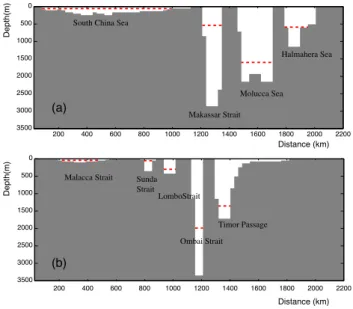
10

As stated above, water from the Pacific flows through the Indonesian Archipelago into the eastern Indian Ocean via a complex series of passages (Fig.1). In the north there are connections with the North Pacific via the shallow southern portion of the South China Sea, the Makassar Strait (sill at 550 m), the Molucca Sea (1600 m) and the Halmahera Sea (500 m). In the east there is an additional connection with the South

15

Pacific via the shallow Torres Strait.

In the south and west, there are connections with the Indian Ocean via the Malacca and Sunda Straits, both of which are shallow, the Lombok Strait (sill 350 m), the Om-bai Strait (2000 m) and the Timor Passage (1400 m). To investigate the flow we have therefore defined two sections, shown in Fig.1, which stretch from Asia to Australia,

20

and together include all of the above passages. The profiles and sill depths of each passage are shown in Fig.2.

Transports are calculated from the model velocity field using the equation,

M₌ Zh z1 d z ZB A d s ∧ v , (1)

where M is the volume transport, z is the vertical coordinate and s the horizontal

25

coordinate running between the two ends of the sectionA and B. The vector v is the 330

(8)

OSD

Full Screen / Esc

velocity,h is the sea surface elevation and z1is the ocean bottom (which is negative). In order to ensure that the result is fully consistent with the model conservation equations, the sections are chosen to follow the edges of the model tracer boxes.

Using the above equation, we calculated the ocean model transports through each passage, and the total for each section, over the full six year analysis period. The

5

transport time series are plotted in Figs. 3 to 7 and the six year and annual averages tabulated in Tables1and2.

2.1 Transports with climatological forcing

When forced by the monthly climatological winds, the mean transport through the northern section during the analysis period is 11.7 Sv. (Unless otherwise stated all

10

transports quoted are from the Pacific towards the Indian Ocean, 1 Sv=106m3s−1). The mean transport through the southern section is 11.8 Sv, the slight difference being due to evaporation and precipitation in the region between the two sections. River flow was not included in OCCAM but if included it would also contribute to the difference.

The transport time series (Fig.3a) shows that the throughflow is highly variable, with

15

both high frequency and year to year variations. Maximum transports occur around June and July and minimum transports around December and January, the total range varying from 5 Sv to 6 Sv depending on the year. The time series also shows that transport dropped slightly during the analysis period, probably due to changing model stratification in the Indian and Pacific Oceans.

20

Table1shows that, in the north, the Makassar Strait is the primary route for the model throughflow, the average transport being 5.7 Sv. There is also a significant annual variation (see Fig. 4) with a maximum of 8 Sv to 9 Sv occurring in July and August. Because it is the westernmost deep passage, the transport through the Makassar Strait is expected to be the largest. However the model results indicate that there are also

25

significant transports via the Molucca Sea (2.1 Sv), the Halmahera Sea (1.6 Sv), and the shallow South China Sea (1.7 Sv).

The transport time series (Fig. 4) also show a wide range of behaviour. In the South China Sea, the transport follows a regular pattern, repeating each year with

(9)

OSD

Full Screen / Esc

a maximum flow of 4 Sv to the south in January and a small, 0.2 Sv, northward flow in June. When Fourier transformed, the data shows an r.m.s. amplitude2 of 1.6 Sv near 1 cy/year. There are additional contributions at 2 and 4 cy/year resulting from the underlying saw-tooth signal.

The South China Sea route is very shallow and so the dynamics is expected to be

5

dominated by the balance between surface wind stress and bottom friction. Thus the strong repeating annual signal seen in the model results is almost certainly a response to the local winds. A similar behaviour is also seen in the transport through Torres Strait, the small annually signal reflecting the fact that the strait is both narrow and shallow.

10

In contrast, a more complicated pattern is seen in the three deep sections. Here the regular annual signal is still present but it is largely masked by an irregular fluctuations with periods near 6 cy/year. If the six-year Makassar Strait time series is Fourier trans-formed, the spectra shows a peak with r.m.s. amplitude of 0.9 Sv at 1 cy/year, a similar peak with r.m.s. amplitude of 0.9 Sv at 2 cy/year, and then a large group of lines with

15

variances of order 0.5 Sv between 5 and 7 cy/year. The spectra for the Halmahera and Molucca passages, show annual (and for Halmahera a semi-annual peak) of compara-ble amplitudes but the peaks around 6 cy/year are much larger, 1.1 Sv for Halmahera and 1.3 Sv for Molucca.

Amongst the Southern sections (Fig. 5), the largest mean transports in the model

20

occur through the Lombok Strait (5.7 Sv) and the deeper Ombai Strait (4.5 Sv). The fluctuations in the transport through the Lombok Strait are dominated by a two cycle per year signal (amplitude 1.2 Sv). In the Ombai and Timor passages there are strong annual and semi-annual signals, Timor having spectral peaks of 1.1 Sv at 1 cy/year and 0.9 Sv at 2 cy/year and Ombai peaks of 0.8 Sv at 1 cy/year and 0.6 Sv at 2 cy/year. All

25

three passages also show irregular fluctuations at shorter periods but the amplitude is much smaller than for the northern sections. Thus for Lombok Strait the fluctuations

2

Quoted r.m.s. values are the square root of the total variance in neighbouring frequency bands.

(10)

OSD

Full Screen / Esc

near 6 cy/year have an r.m.s. amplitude of 0.5 Sv and Ombai and Timor Straits both have values near 0.3 Sv.

The fact that the fluctuations with periods near 6 cy/year are irregular implies that they are associated with waves propagating through the ocean and that they are not due to the local repeating winds. The differences between the spectra for the northern and

5

southern passages also imply that the waves responsible for the enhanced energies in the north do not propagate through the Indonesian Archipelago. Thus if, at one instant, the waves produce an enhanced inflow through one northern passage this must be compensated by an outflow though the other northern passages.

2.2 Transports with high-frequency forcing

10

In the second run, when the model is forced by the more realistic ECMWF analysed winds, there are significant changes in both the mean transports and their variability. The total mean throughflow, averaged over the six years, increases from 11.7 and 11.8 Sv to 12.9 Sv and 13.0 Sv through the northern and southern sections respectively. The time series (Fig.3b and Table2), shows that the largest values of the throughflow

15

occurred between 1994 and 1996, the annual average reaching 14.9 Sv through the northern section in both 1994 and 1995. This is followed by a sharp drop to 10.2 Sv in 1997 and 10.9 Sv 1998. Both years were partly affected by an El Nino. The SOI index was large and negative between April 1997 and April 1998, but the model indicates that the throughflow was reduced over a much longer period of time.

20

In the north, the Makassar Strait is the primary route for the throughflow with a mean transport over the six year period of 5.9 Sv. The maximum flows, up to 10 Sv, occur in July and August and the minimum, as low as 2 Sv, in January and February.

The next most important route in the model is via the Halmahera Sea, where the mean transport is 3.4 Sv. This is 1.8 Sv more than that found with monthly averaged

25

winds. Maximum southward flows, around 6 Sv, occur in October and November dur-ing the Northwest Monsoon. Minimum flows, can in practice be northward flows, the northward transport during January and February 1997 averaging 2 Sv. There are also significant transports via the shallow South China Sea (average of 1.2 Sv) and the

(11)

OSD

Full Screen / Esc

Molucca Sea (1.8 Sv). Year to year variability is significant (Table2), the Halmahera Sea transport ranging from 5.9 Sv in 1994 to −0.44 Sv (i.e. northwards) in 1998.

There is also a large increase in variability at shorter periods although the annual signal (see Fig. 3) still appears coupled to the monsoon. Between 1993 and 1996 maximum maximum monthly values, up to 21 Sv, occur in in June, July and August and

5

minimum values around 10 Sv in December and January. The El Nino years of 1997 and 98 have lower transports, the monthly average throughflow being below 5 Sv in January 1998.

Amongst the northern sections, the largest amount of short term variability is found in the Molucca Passage. The Makassar and Halmahera passages also show significant

10

variability but in the two shallow sections, the South China Sea and Torres Strait, short term variability is small.

Amongst the southern sections, the largest mean transports occur through the Lom-bok Strait (5.6 Sv) and the Ombai Strait (4.9 Sv). Next most important is the Timor Passage, its average transport, (2.2 Sv), being almost twice that found with the monthly

15

wind forcing run. All three passages also show significant short term variability, but the amplitude is less than that seen in the deep northern passages.

3 Vertical structure

The vertical distribution of transport was calculated from the OCCAM model velocity field using the equation,

20

T1= ZB1

A₁ d s ∧ u

1(δz1+ h0)/δz1, (2)

for the shallowest model level, and,

T_i = ZBi

Ai

d s ∧ ui, (3)

(12)

OSD

Full Screen / Esc

for the deeper levels, where T_i is the transport per unit depth at level i , ui the mean

velocity, δzi the level thickness, h0 the sea surface elevation and s is the horizontal coordinate along the section. The resulting vertical distribution of the mean (six-year average) transports are show in Figs.8to11.

3.1 Monthly climatological wind run

5

The total transports per unit depth for the northern section of the monthly climatology wind forced run is shown in Fig.8 together with the transport through the individual passages. The total transport is concentrated mainly in the top 500 m and it has a sub-surface maxima at approximately 100 m depth. Below 500 m the transport per unit depth remains fairly uniform down to 1100 m. There is then a weak flow reversal, down

10

to 1700 m, followed by a weak flow out of the Pacific down to 2000 m.

The data for the individual passages shows that the most of the flow above 400 m is through the Makassar Strait. This has a sub-surface maximum (around 120 m) and then drops off rapidly, with little flow below 400 m and none below 600 m. Below 400 m, largest transports are found through the Molucca Strait, and this is responsible for all of

15

the transports below 600 m. This is to be expected as it is the only passage with a sill below 550 m. Above 500 m the flows through the Molucca Strait are negligible, except for a slight flow reversal in the top 100 m.

Near the surface the flows through other sections in the north also become signifi-cant. In the case of the S China Sea, this may be expected because of the effect of the

20

monsoon on the shallow waters of the region. The beta effect may also be involved, steering any steady current from the North Pacific into the Indian Ocean as far west as possible. However the model also shows significant flow through the Halmahera Sea. This extends down to at least 200 m, is unexpected, and indicates that other factors are involved.

25

The corresponding transports for the southern sections are shown in Fig. 9. The total transport shows two important changes. First the sub-surface maximum has dis-appeared and instead the maximum transport per unit depth occurs at the surface. Secondly there is a weak deep circulation, with flow out of the Indian Ocean between

(13)

OSD

Full Screen / Esc

1200 m and 2100 m and a return flow below that down to 3200 m.

Above 300 m the bulk of the flow is through the Lombok Strait. (This is a fault of the model which is discussed later). The flow has a maximum at the surface and then drops off rapidly with depth. Next in importance is the Ombai Strait. This has a slight near surface maximum, but otherwise the flow is relatively constant down to 1100 m.

5

Below 300 m almost all the transport goes via this route. It is also responsible for all of the weak deep circulation below 1200 m.

3.2 High frequency forcing

The vertical distribution of transport with actual six-hourly wind forcing is shown in Figs.10and11. The gross features are the same as for monthly forcing – except for the

10

surface layer where there are significantly increased transports through the Halmahera Strait in the north and through the Ombai and Timor Straits in the south. The six-hourly wind run also produces a reduction of the deep flows through the Ombai Strait.

It is not obvious why the vertical profiles differ in the two runs. The monthly climato-logical run was based on winds for the period 1986–1988, whereas the analysis period

15

for the actual six-hourly wind run covers the period 1993–1998. Thus the differences in the mean winds over these periods may be responsible. However the actual winds may vary very rapidly, so it is possible that non-linearities acting on the short term wind driven fluctuations may also produce the observed changes in the averaged current.

4 Godfrey’s Island Rule

20

In his study of the Global Ocean Circulation,Godfrey (1989,1996) developed a new method for estimating the average total northward transport of the South Pacific Ocean between Australia and South America. The method involves an integral of the time average wind stress along a path which includes two east-west crossings of the South Pacific, at the northern and southern extremities of the Australian and New Guinea

25

continental shelf. These two east-west sections are then joined by paths along the shelf edges of South America and West Australia.

(14)

OSD

Full Screen / Esc

Godfrey’s estimate of the transport, which has become known as Godfrey’s Island Rule, is given by the equation:

T_o= I

τ · d s/ρo(fN− fS), (4)

whereT_ois the total depth-integrated mass transport, τ is the time average wind stress,

s _{is the locus of the path of integration,} _ρ

o is the mean water density, andfN−fS are

5

the values of the Coriolis parameter at the latitudes of the two east-west.

If the Island Rule is valid then it should equal the Indonesian Throughflow plus any transport through the Bering Strait and the effect of evaporation, precipitation and river inflow in the North Pacific. In practice the mean northward transport through the Bering Strait is about 1 Sv and precipitation, evaporation and river inflow also contribute about

10

1 Sv. In the following we assume that these terms cancel out.

Pirani(1999) used results from the climatological wind run to carry out a preliminary

comparison of the model throughflow with the value predicted by Godfrey’s Island Rule. The integral path was approximated by a rectangle with boundaries at the equator, 115◦_{E, 40}◦_{S and 85}◦_{W and comparisons were made for model years nine to twelve}

15

inclusive of the run. Godfrey’s Rule is based on Sverdrup transport ideas, which are really concerned with the long term mean transport of the ocean after all transient waves have died out. However Pirani’s results showed that there was good agreement for both the mean transport each year and the annual cycle. This implies that there may be more to be gained from the integral, for example as an analogue of the time

20

varying Indonesian Throughflow.

For the present study we calculated the integral in Eq. (4) using the more accurate path shown in Fig.12. The path is similar to the one used by Godfrey but, to the west of Australia and South America, it follows the continental shelf edge at a depth of 100 m. No correction has been made for New Zealand as Godfrey found that its effect was

25

negligible.

Comparisons were made for years nine to fourteen for run CMW and years 1993 to 1998 for run E6W. For each year we calculated the mean transports and the amplitude

(15)

OSD

Full Screen / Esc

of the annual, semi annual and higher frequency signals. The results are given in Tables3and 4, together with the response, that is the ratio of the actual transport to the value predicted by the Island Rule and the phase delay between the maximum in the wind forcing and the maximum in the transport.

The results from the climatological forcing run agree with those of Pirani. The mean

5

value of the throughflow each year is given to a good approximation by the Godfrey Island rule. The annual signal, which can be seen in Fig.3, is also in good agreement for both the amplitude and phase. At higher frequencies the agreement is poor, the actual variation being much smaller than the value predicted by the Godfrey formula.

With the six-hourly winds there is much more variability in both the observed

trans-10

ports and the Godfrey predicted value. Averaged over the six years, the model through-flow agrees well with the Godfrey prediction. However in individual years (Table4), both the mean transports and the ratio vary significantly, indicating that the Island Rule by itself is not suitable as an analogue of the annual mean transports.

Figure 3 indicates that the annual signal is larger in the six-hourly run than in the

15

climatological run, but its peak occurs at about the same time during the year. This is confirmed by Fourier analysis (see Table4) which also shows that the Godfrey Island Rule has some skill in predicting the amplitude and phase of the transport especially between 1993 and 1996.

Smoothed versions of the two timeseries (Fig.13) also show better agreement

be-20

tween between 1993 and 1996 than for the two El Nino years, 1997 and 1998. The Island Rule is based on the steady state solution after all gravity and Rossby waves have propagated around the system and died away. The present results thus indi-cate that the energetic waves generated by the El Nino are taking longer to propagate through the system than the normal annual variations seen earlier.

25

When calculating the response values, we hoped to find evidence that propagation delays were responsible for the differences between the two time series. However we could find no evidence for this, either in the analysis of individual years (Table4) or in a combined analysis of the whole six-years.

(16)

OSD

Full Screen / Esc

5 Comparison with observations

The analysis so far has concentrated on the behaviour of the model ocean under the two forcing regimes. In this final section on the analysis, the focus is on how well the model reproduces know aspects of the real ocean. The best set of data available for the region is hydrographic data and this is considered first. There is also an important set

5

of current meter measurements which have been used to estimate transports through some of the straits.

The comparisons show up a number of apparent failings of the model. Most seem to be the result of errors in the model physics but there are some where the model may be partially correct. In any case the results are a stimulus – both to improve the model

10

and to improve our limited physical understanding of the flows. 5.1 The water masses

The Indonesian Throughflow transports an important group of water masses from the North Pacific into the Indian Ocean. Within the region, the deep basins also give rise to a series of remarkably uniform water masses. In order to illustrate how well the model

15

represents such features, Fig. 14 shows the average summer temperatures during years nine to fourteen of the monthly climatological wind forced run along a section through the eastern side of the Indonesian Archipelago. The section is similar to that used by Wyrtki (1961) in reporting observations from the region (see his Fig. 6.25, also based on summer data), and by van Aken et al. (1988) in their report on later

20

measurements. TheLevitus and Boyer(1994a) summer temperatures, plotted for the same section in Fig.15, lie close to the values given in the two observational papers.

Comparison of the different figures shows that above 1200 m, at the levels with the largest transports, there is reasonable agreement between the model and observa-tions. Below 1200 m the flow is blocked by sills. The resulting water properties therefore

25

reflect the actual water mass overflowing each sill and the mixing processes occurring within the sill regions and the deep basins.

In the deep Pacific and Indian Oceans the model temperature profiles are little 339

(17)

OSD

Full Screen / Esc

changed from the initial state and so are in reasonable agreement with observations. In the deep Indonesian Basins, the bottom temperatures in the model also compare well with observations, warming slowly in going from the Pacific to the Indian Ocean. However in the vertical, the temperature gradient is much weaker than it should be. As a result, the deep basins are capped by a much stronger thermal gradient than is

5

observed in the real ocean.

This result was unexpected. Ocean models like OCCAM, which use level surfaces, tend to produce too much vertical mixing in the open ocean, because of numerical effects and because of internal waves which mix water up and down between model layers. These effects should mix down additional heat from the surface layers,

weak-10

ening the thermocline and warming the deep basins. Mixing in the poorly represented overflows would also tend to increase the model temperatures at depth.

We investigated the Banda Sea region and concluded that the error there arose primarily because of model errors at the Lifamatola Strait (1◦₁₀′_{S, 126}◦₄₉′_{E). This lies} at the southern end of the Molucca Sea. It is the deepest sill connecting the Banda

15

Sea to the Pacific Ocean and is deeper than any of the routes connecting the Banda Sea with the Indian Ocean.

A detailed survey of the strait (van Aken et al.,1988), showed that the overflow region is roughly V-shaped in profile and that it has a sill depth that lies between 1950 m and 2000 m. Below 1900 m the strait is less than 2 km wide, at 1700 m it is approximately

20

5 km wide and at 1500 m approximately 20 km wide. Current measurements in the strait showed that the transport was 1.5 Sv and temperature profiles downstream showed that the overflow forms a “quasi-homogeneous layer” with a thickness of about 500 m, which continues downslope to depths near 3000 m (van Aken et al.,1991).

In the model, the Lifamatola Strait is represented with a sill at 1823 m. During the

25

analysis period all the southward flow was confined to the bottom layer (extending from 1823 m to 1615 m). The transport in the layer was 0.8 Sv and the temperature was approximately 2.5◦C. The transport is less that that observed but the temperature is approximately equal to the average temperature of the overflow observed byvan Aken

(18)

OSD

Full Screen / Esc

et al. (1988). It is also similar to the temperature in the offshore Pacific at this depth. Near the sill, at a depth of 1950 m, van Aken et al. (1988) observed temperatures of 2.3◦C but bottom temperatures rose to 2.4◦C only a few kilometers downstream. Further downstream, the minimum temperature in the Baru Basin is approximately 2.6◦_{C and in the Banda Sea itself the minimum observed temperatures lie near 2.78}◦_C

5

(Wyrtki,1961).

Both the observations and the model are thus consistent with the inflow of Pacific waters in a layer, possibly a few hundred metres thick, with average temperatures near 2.5◦C. There is then some turbulent mixing in the overflow which produces warmer temperatures at the bottom of the Baru Basin and the Banda Sea.

10

This does not explain why, during the analysis period, both the transport in the over-flow and the density profile in the deep basins are so weak. However further study indicates that both effects arise because the model sill is far too wide. As the model uses a grid spacing of 1/4◦_{, the sill has a width of one velocity grid box (27.8) km and} two tracer grid boxes (55.6 km). The increased number of tracer boxes arises from

15

the staggered grid used by the Arakawa-B scheme. As a result the overflow is best thought of as having a velocity profile in the horizontal which is triangular in shape, with a maximum in the centre and a width of 55.6 km.

If we assume that the average width of the actual sill is given by the value at 1700 m, then the model sill has a cross sectional area which is eleven times too large.

Dur-20

ing the analysis period the transport in model is low but this is only after the presure difference between the Pacific and the Banda Basin has almost equalised (it is then equivalent to a dynamic height difference of 0.25 cm). During year 4 of the run, the earliest available for analysis, the transport was much higher (3.6 Sv). The dynamic height difference (1.0 cm) was also higher and presumably more realistic.

25

The large width of the model sill also means that the viscous terms are underesti-mated. The horizontal viscosity term is proportional to the width squared, so even after allowing for the excess length of the channel (two velocity boxes, so possibly a factor of three too long), the viscosity term in the model is still likely to be a factor of 40 too

(19)

OSD

Full Screen / Esc

small. Analysis of the momentum balance in the sill regions showed that both at year 4 and during the main analysis period, the viscosity term was a factor of 10 smaller than the along channel pressure gradient3. With a realistic channel width the total transport would be reduced and the viscous term could thus become significant.

In their analysis of their results, van Aken et al.(1991) concluded that the vertical

5

structure of the Banda Sea resulted from the balance between vertical mixing within the basin and the influx of the bottom waters by the inflow through the Lifamatola Strait. A flow of 1.5 Sv gives a flushing time of about 27 years, so if this is increased to 3.6 Sv or more, as occurred early in the model run, it would significantly affect the stratification after only a few years.

10

We conclude that the wide model sill resulted in a large inflow of dense water from the Pacific which filled the deep Banda Sea Basin early in the run. This produced a more uniform water mass in the deep basin. As the basin filled with denser water it also reduced the pressure gradient across the sill, reducing the inflow until the model transport was less than that observed.

15

In future models, a better representation of sills is required. This could be done by using a finer horizontal grid. An alternative is to use partial box widths, in the same way that partial box depths are presently used to obtain a better mean ocean topography. The channel width also affects the viscosity terms in the momentum equation. Thus the viscosity terms will also need correcting.

20

5.2 Current meter observations and transports

A further check on the model comes from transports estimated from the limited current meter data. In the north there have been moorings in the Makassar Strait from De-cember 1997 to July 1998 (Gordon et al.,1999;Susanto and Gordon,2005) and the Lifamatola Passage overflow, at the southern end of the Molucca Sea, from January to

25

March 1985 (van Aken et al.,1988,1991).

3

The horizontal pressure gradient is balanced primarily by the inertial terms in the along-channel momentum equation. This is as expected when a control point is involved.

(20)

OSD

Full Screen / Esc

In the south there have been measurements in the Lombok Strait from January 1985 to January 1986 (Murray and Arief,1988;Murray et al.,1990;Arief and Murray,1996), in the Timor Passage from August 1989 to September 1990 and from March 1992 to April 1993 (Cresswell et al.,1993;Molcard et al.,1994,1996), and in the Ombai Strait from November 1995 to November 1996 (Molcard et al.,2001).

5

There have also been some indirect estimates of transports. Meyers (1996) used XBT sections andFieux et al. (1996) hydrographic data from sections between Aus-tralia and Indonesia. Transports depended strongly on season and varied between 2.6±9 Sv and 18±7 Sv.Qu(2000) used hydrographic data to estimate the flow through the Luzon Strait (3 Sv), most of which will have turned south through the shallow S

10

China Sea. Wolanski et al.(1988) studied the flow through Torres Strait and found a transport of order 0.01 Sv..

In his review of the transport estimates, Gordon (2005) concluded that the mean value for the total transport lies in the range of 8 to 14 Sv, his preferred value being about 10 Sv. The OCCAM model transports reported here (11.7 Sv for run CMW and

15

12.9 Sv for E6W) are thus within the overall limits but on the high side of his preferred value.

If we compare individual straits the agreement is not so good. In the north the most striking difference is in the Makassar Channel, where the model gives values of 5.7 and 5.9 Sv for the two runs. These are lower than Susanto and Gordon’s (2005) estimate of

20

7 to 11 Sv. There is also a marked difference in the Halmahera Sea where the model shows transports of 1.6 and 3.4 Sv. Gordon (2005) assumed the transport here was negligible butCresswell and Luick(2001) using a single mooring found a transport of 1.5 Sv at depths between 350 m and 700 m. Unfortunately, in the model this channel is blocked at these depths so flow only occurs above 300 m. However both observations

25

and model indicate this may be a significant pathway.

Between the two straits lies the Malacca Strait with its sill at the Lifamatola Strait.

van Aken et al.(1991) estimated a transport of 1.5 Sv in the overflow and implied that

after mixing and upwelling this continued as part of the throughflow. In the model there 343

(21)

OSD

Full Screen / Esc

is an overflow, as discussed in the previous section, but the upwelled water returns to the Pacific (see Fig.14). This is because the sill to the Indian Ocean lies at a much shallower depth (1420 m). Above 1000 m the model shows a second region of inflow through the Malacca Strait which continues through to the Indian Ocean.

In the south, the most striking difference between the model and observations occurs

5

in the Lombok Strait. Murray and Arief(1988) found a transport of of 1.7 Sv concen-trated in the upper 200 m. The model finds much larger values, 5.7 Sv and 5.6 Sv for the two runs but agrees that these are concentrated in the top 200 m.

Further east observations in the Timor Passage (Cresswell et al.,1993;Molcard et

al.,1994,1996) give transports of 3 to 6 Sv, the model much lower values of 1.1 and

10

2.1 Sv. For the Ombai Strait,Molcard et al. (2001) estimate 4 to 6 Sv, the model 4.5 and 4.9 Sv. The model thus seems to increasing the near surface flows in the Lombok Strait at the expense of the Timor Passage.

5.3 The deep western channels

In studying these discrepancies we have concentrated on the two deep western

chan-15

nels, the Makassar Strait where the model transport appears to be too low and the Lombok Strait where it appears to be too high. At the surface, the Makassar Strait appears to be very much wider than the Lombok Strait, but it is blocked by sediments at its southern end, so that below 30 m the width is reduced to about 25 km.

The Lombok Strait has a similar width over most of its length, but around 115◦45′E,

20

8◦46′S, near the island of Paula Penida, it narrows to 13 km for a distance of under 20 km. As with the Lifamatola Sill, the width at the narrows is less than the model grid, so the extra model transport may be partially explained by the differing cross-sectional area at the narrowest point.

The model is also likely to be underestimating the effect of viscosity in the strait. In

25

the model, the magnitude of the horizontal viscous forces acting on the top 200 m is equivalent to a pressure difference of approximately 0.4 cm between the ends of the strait. In comparison, the average dynamic height difference along the western bound-ary at this depth is 3 cm. Thus in the model, viscosity appears to have little effect on the

(22)

OSD

Full Screen / Esc

flow. However if it were increased by a factor of four or more, its effect should become significant. This would happen if the width of the strait was correctly represented in the model. Internal tides and other features of the flow may also increase the viscosity in the region.

The low model transport in the Makassar Strait is not so easily understood. The

5

narrowest section, the Labani Channel (3◦0′S, 118◦40′E) is about 28 km wide4 and 70 km long, so it is reasonably well represented by the model. The viscous terms, at year 10.0 in run CMW, correspond to a dynamic height difference of 0.6 cm. This is much smaller than the actual difference in dynamic height between the ends of the Labani Channel (3 cm at a depth of 100 m).

10

Both here and in the Lombok Strait, the difference is consistant with a horizontal control point acting on the surface layers of the channel. Such control points have been discussed byArmi and Williams (1993). The strong accelerations at the entrance to the channel and the shallowing of the density surfaces in passing through the channel give support to this conclusion. If so, it is possible that the model is providing too much

15

control on the flow in the Labani Channel. This may be due to finite-difference effects in the model but, whatever the explanation, the effect must be subtle in order to explain why similar constrictions produce too much flow in the Lombok Strait and too little in the Makassar Strait.

Having failed to explain the behaviour in terms of small scale model physics, we also

20

looked at the larger scale. If Godfrey’s theory is correct and the throughflow is primarily generated by the northward flow in the South Pacific, then the shortest route to the Indian Ocean is via the Halmahera Sea. In order to follow the ’deep western boundary current’ route via the Makassar Strait, the flow would have to go a few degrees further north. At mid-latitudes any blockage like this normally causes the current to split (Webb,

25

1993). So if Godfrey is correct, the throughflow should generate flows through both the Halmahera Sea and the Makassar Strait – as seen in the model.

4

Wajsowicz at al. (2003), Fig. 9, show that the channel is just under 50 km wide at their

mooring position.

(23)

OSD

Full Screen / Esc

6 Discussion

The Indonesian region has an important role in the large scale circulation of the ocean. It therefore needs to be accurately represented in many types of ocean model, ranging from the high resolution ocean physics models, to the medium resolution biological models and the low resolution ocean models used in climate change research. Over

5

the next ten years, most ocean models are likely to use a resolution similar to or lower than the one used here. The results of the present work should thus be relevant to all such models.

The present analysis has shown a number of areas where the model agrees roughly with expectations. Rather more interresting are the areas where the model fails and

ar-10

eas where it throws up questions whose solution seems to require better observations and the development of better theories.

We have shown that after nine years with climatological winds, the total throughflow agrees with observations and, to within a few percent, with the value predicted by God-frey’s Island Rule. Using the more realistic ECMWF winds we found that the model and

15

Godfrey’s Island Rule roughly agree at a period of one cycle per year. They disagree at shorter periods, which one might expect, but they also give different values for the year to year variations in transport. To us it seems odd that both the long term and annual wind fields give agreement between the model and Godfrey’s Island Rule but that at intermediate frequencies the agreement breaks down. The results invite further study.

20

One promising approach is that ofLee et al. (2001). He used an adjoint model to show that at periods of a year, the throughflow is affected by winds in the western equatorial Pacific and by winds south of Australia. Both regions lie near the path of the Godfrey Integral and so help to explain the correlation seen here. It would be interesting to use an adjoint model to investigate the relationships at other frequencies.

25

When we investigate the spectra, we find that the spectra of the flows through the in-dividual northern straits differ significantly from the spectra through the southern straits (although the spectra for the total flows are similar). It raises the question as to whether

(24)

OSD

Full Screen / Esc

the region acts as a filter stopping waves progressing through the region. This could be a latitude effect, although the southern end of the Makassar Strait is very similar in latitude to the Lombok Strait. Again the topic invites further study.

In the deep basins we found that although the deep temperatures were reasonable, the vertical stratification was too weak. This was traced to errors in the sills, especially

5

the Lifamatola Sill which was far too wide. Part of the problem could be solved by introducing partial box widths, as well as the partial bottom box depths that are used in current ocean models. However the V-shaped sill region is much more complex than is usually allowed for in ocean models and raises the question of what improvements are needed before the models can accurately represent the effect of critical points, mixing

10

and other aspects of the overflows.

The model also raised the question of what happens to the deep water upwelled in the Banda Sea and surrounding basins. Usually it is assumed that this continues upwelling within the region until it is shallow enough to continue on into the Indian Ocean. However, the model results suggest that it is a lot easier for the upwelled water

15

to return to the Pacific. If in reality this does not happen, we need to understand why. The model flow through the Lombok Strait was much larger than the observations. The reason is again probably due to the channel width being too large in the model. The representation of viscosity in the model and the extra effects of locally generated turbulence in the strait could also be involved. For many purposes an “engineering” fix

20

can be used in which viscosity is increased5or a partial box width is used. However as with the overflows it is not obvious that this will correctly represent the effect of changes in the flow. Better observations, better theories and better model parameterisations are all needed.

Finally the model gave lower transports through Makassar Strait than were expected,

25

and larger transport through the Halmahera Sea. We are unable to explain the discrep-ancy although, as discussed, in both cases horizontal control points may be involved. The possibility needs to be explored further.

5

As used in other models, (G. Madec, private communication)

(25)

OSD

Full Screen / Esc

If the long term mean throughflow is determined by the Godfrey Island Rule then we would expect the northward flow in the S Pacific to take the shortest route to the Indian Ocean. This would involve a current along the north coast of New Guinea which, on approaching Halmahera, is likely to split. Part would turn south into the Halmahera Sea and part turn north to eventually join the Makassar Strait current.

5

It is possible that this is what happens. If so then the observations of Cresswell

and Luick (2001) may be significant but why are the Makassar transport estimates so large? If the theory is not correct then why not? In either case some key part of the observations or the theory appears to be missing. Further research is required.

Acknowledgements. We wish to thank B. de Cuevas and A. Coward for their valuable work with

10

the OCCAM model and for their technical support and helpful comments during the period of this research.

References

Arakawa, A.: Computational design for long-term numerical integration of the equations of fluid

motion: Two-dimensional incompressible flow, J. Comput. Phys., 1, 119–143, 1966. 328

15

Arief, D. and Murray S. P: Low-frequency fluctuations in the Indonesian Throughflow through

Lombok Strait, J. Geophys. Res., 101(C5), 12 455–12 464, 1996. 343

Armi, L. and Williams, R.: The hydraulics of a stratified fluid flowing through a contraction, J.

Fluid Mech., 251, 355–375, 1993.345

Bryan, K.: A numerical method for the study of the circulation of the world ocean, J. Comput. 20

Phys., 4, 347–376, 1969. 328

Bryden, H. L. and Beal, L. M.: Role of the Agulhas current in Indian ocean circulation and associated heat and freshwater fluxes, Deep-Sea Res., 48, 1821–1845, 2001.

Cox, M. D.: A primitive equation 3-dimensional model of the ocean, Tech.Rep. 1, Geophysical Fluid Dyn. Lab, Natl. Oceanic and Atmos. Admin., Princeton Uni. Press, Princeton, N.J., 25

1984. 328

Cresswell, G., Frische, A., Peterson J., and Quadfasel, D.: Circulation in the Timor Sea, J.

Geophys. Res., 98, 14 379–14 389, 1993. 343,344

(26)

OSD

Full Screen / Esc

Printer-friendly Version Interactive Discussion Cresswell, G. R. and Luick J. L.: Current measurements in the Halmahera sea, J. Geophys.

Res., 106, 13 945–13 951, 2001. 343,348

Fieux, M., Molcard, R., and Ilahude, A. G.: Geostrophic transport of the Pacific-Indian Ocean

throughflow, J. Geophys. Res., 101(C5), 12 421–12 432, 1996. 343

Godfrey, J. S.: A Sverdrup model of the depth-integrated flow for the world ocean allowing for 5

Island circulations, Geophys. Astrophys. Fluid Dyn., 45, 89–112, 1989. 328,336

Godfrey, J. S.: The effect of the Indonesian Throughflow on ocean circulation and heat ex-change with the atmosphere: A review, J. Geophys. Res., 101(C5), 12 217–12 237, 1996.

327,328,336

Gordon, A. L.: Oceanography of the Indonesian Seas and their Throughflow, Oceanography, 10

18(4), 14–27, 2005. 327,343

Gordon, A. L., Susanto, R. D., and Ffield, A.: Throughflow within Makassar Strait, Geophys.

Res. Lett., 26, 3325–3328, 1999. 342

Griffies, S. M., Gnanadesikan, A., Dixon, K. W., Dunne, J. P., Gerdes, R., Harrison, M. J., Rosati, A., Russell, J. L., Samuels, B. L., Spelman, M. J., Winton, M., and Zhang, R.: For-15

mulation of an ocean model for global climate simulations, Ocean Sci., 1, 45–79, 2005,

http://www.ocean-sci.net/1/45/2005/. 328

Hellerman, S. and Rosenstein, M.: Normal monthly wind stress over the world ocean with error estimates, J. Phys. Oceanogr., 13, 1093–1104, 1983.

Lee, T., Giering, R., and Cheng, B.: Adjoint sensitivity of Indonesian throughflow transport 20

to wind stress: application to interannual variability, Jet Propulsion Laboratory Publication

01-11, 36 pp, 2001. 346

Levitus, S.: Climatological atlas of the world ocean, NOAA Professional Paper No 13, GFDL,

Princeton University, NJ., 1982. 329

Levitus, S. and Boyer, T. P.: World Ocean Atlas 1994. NOAA Atlas NESDIS, Volume 4, Tem-25

perature, 117pp., 1994a.329,339

Levitus, S., Burgett, R., and Boyer, T. P.: World Ocean Atlas 1994, NOAA Atlas NESDIS,

Volume 3, Salinity, 99pp., 1994b. 329

Molcard, R., Ilahude, A. G., Fieux, M., Swallow, J. C., and Banjarnahor, J.: Low frequency variability of the currents in Indonesian Channels (Savu-Roti M1 and Roti-Ashmore Reef 30

M2), Deep Sea Res., 41, 1643–1662, 1994. 343,344

Molcard, R., Fieux, M., and Ilahude, A. G.: The Indo-Pacific Throughflow in the Timor Passage,

J. Geophys. Res., 101, 12 411–12 420, 1996. 343,344

(27)

OSD

Full Screen / Esc

Printer-friendly Version Interactive Discussion Molcard, R., Fieux, M., and Syamsudin, F.: The Throughflow within Ombai strait. Deep-Sea

Research, 48(5), 1237–1253, 2001. 343,344

Murray, S. P. and Arief, D.: Throughflow into the Indian Ocean through the Lombok Strait,

January 1985–January 1986, Nature, 333, 444–447, 1988.343,344

Murray, S. P., Arief, D., Kindle, J. C., and Hurlburt, H. E.: Characteristics of circulation in an 5

Indonesian Archipelago Strait from hydrography, current measurements and modelling re-sults, in: The Physical Oceanography of Sea Straits, edited by: Pratt, L., Kluwer Academic

Publishers, Norwell, MA, pp. 3–23, 1990.343

Meyers, G.: Variation of Indonesian throughflow and the El Ni ˜no-Southern Oscillation, J.

Geo-phys. Res., 101, 12 255–12 263, 1996. 343

10

Pacanowski, R. C. and Philander S. G. H.: Parameterization of vertical mixing in numerical

models of tropical oceans, J. Phys. Oceanogr., 11, 1443–1051, 1981. 329

Pirani, A.: Testing Godfrey’s Island Rule using the OCCAM model for the calculation of the

Indonesian Throughflow. MSc Thesis, University of Southampton, 1999. 337

Qu, Tangdong: Upper-Layer Circulation in the South China Sea, J. Phys. Oceanogr., 30, 1450– 15

1460, 2000. 343

Semtner, A. J.: An oceanic general circulation model with bottom topography. Technical Report

No. 9, Dept of Meteorology, UCLA, Los Angeles, CA 90095, 1974. 328

Siefridt, L. and Barnier, B.: Banque de Donnes AVIS Vent/flux: Climatologie des Analyses de

Surface du CEPMMT, ORSTOM Report 91 1430 025, Toulouse, 1993.329

20

Susanto, R. D. and Gordon, A. L.: Velocity and transport of the Makassar Strait throughflow, J.

Geophys. Res., 110, C01005, doi:10.1029/2004JC002425, 2005. 342,343

Thompson, S. R.: Sills of the global ocean: a compilation, Ocean Modelling, 109, 7–9, 1995. 329

U.S. Naval Oceanographic Office and the U.S. Naval Ocean Research and Development Activ-25

ity: DBDB5 (Digital Bathymetric Data Base-5 Minute Grid), U.S.N.O.O., Bay St. Louis, 1983. 329

van Aken, H. M., Punjanan, J., and Saimima, S.: Physical aspects of the flushing of the East

Indonesian basins, Netherlands J. Sea Res., 22, 315–339, 1988. 339,340,341,342

van Aken, H. M., Van Bennekom, A. J., Mook, W. G., and Postma, H.: Application of Munk’s 30

abyssal recipes to tracer distributions in the deep waters of the southern Banda basin,

Oceanologica Acta, 14(2), 151–162, 1991.340,342,343

Wajsowicz, R. C.: The circulation of the depth-integrated flow around an island with application

(28)

OSD

Full Screen / Esc

to the Indonesian Throughflow, J. Phys. Oceanogr., 23, 1470–1484, 1993. 328

Wajsowicz, R. C., Gordon, A. L., Ffield, A., and Susanto, R. D.: Estimating Transport in Makasar

Strait, Deep-Sea Res. II, 50, 2163–2181, 2003. 345

Webb, D. J.: A simple model of the effect of the Kerguelen Plateau on the strength of the

Antarctic Circumpolar Current, Geophys. Astrophys. Fluid Dyn., 70, 57–84, 1993. 345

5

Webb, D. J.: The vertical advection of momentum in Bryan-Cox-Semtner ocean general

circu-lation models, J. Phys. Oceanogr., 25(12), 3186–3195, 1995. 329

Webb, D. J., de Cuevas, B., and Richmond, C.: Improved advection schemes for ocean models,

J. Atmos. Oceanic Technol., 15, 1171–1187, 1998a. 328

Webb, D. J., de Cuevas, B. A., and Coward, A. C.: The first main run of the OCCAM global 10

ocean model, Internal Report of James Rennell Divesion, Southampton Oceanography

Cen-tre, UK., 1998b. 329

Wolanski, E., Ridd, P., and Inoue, M.: Currents through Torres Strait, J. Phys. Oceanogr., 18,

1535–1545, 1988. 343

Wyrtki, K.: NAGA Report Volume 2. Scientific results of marine investigations of the South 15

China sea and the Gulf of Thailand 1959–1961. Physical Oceanography of the Southeast

Asian Water, Scripps Institution of Oceanography, 195 pp., 1961. 341

(29)

OSD

Full Screen / Esc

Printer-friendly Version Interactive Discussion Table 1. The transports through the northern and the southern sections. Positive transports

correspond to flow from the Pacific Ocean to the Indian Ocean. (1 Sv=106m3s−1_).

Mean Transport (Sv)

Section Width Depth Sill Monthly ECMWF

(km) (m) Depth Winds Winds

(m) Years 9–14 93–98 S. China Sea 1000 240 40 1.7 1.2 Makassar Strait 160 2800 550 5.7 5.9 Molucca Sea 250 2200 1,600 2.1 1.8 Halmahera Sea 230 1150 500 1.6 3.4 Torres Strait 140 20 20 0.6 0.6 Total 11.6 12.9 Malacca Strait 350 100 20 0.2 0.1 Sunda Strait 100 350 20 0.3 0.2 Lombok Strait 80 430 350 5.7 5.6 Ombai Strait 80 3400 2000 4.5 4.9 Timor Passage 520 1800 1400 1.1 2.2 Total 11.7 13.0 352

(30)

OSD

Full Screen / Esc

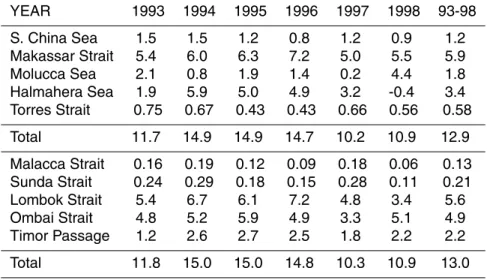
Table 2. Average transports for each strait and for each year when the model is forced by

analysed ECMWF winds. Positive transports correspond to flow from the Pacific Ocean to the

Indian Ocean. Transports in Sverdrups (1 Sv=106m3s−1).

YEAR 1993 1994 1995 1996 1997 1998 93-98 S. China Sea 1.5 1.5 1.2 0.8 1.2 0.9 1.2 Makassar Strait 5.4 6.0 6.3 7.2 5.0 5.5 5.9 Molucca Sea 2.1 0.8 1.9 1.4 0.2 4.4 1.8 Halmahera Sea 1.9 5.9 5.0 4.9 3.2 -0.4 3.4 Torres Strait 0.75 0.67 0.43 0.43 0.66 0.56 0.58 Total 11.7 14.9 14.9 14.7 10.2 10.9 12.9 Malacca Strait 0.16 0.19 0.12 0.09 0.18 0.06 0.13 Sunda Strait 0.24 0.29 0.18 0.15 0.28 0.11 0.21 Lombok Strait 5.4 6.7 6.1 7.2 4.8 3.4 5.6 Ombai Strait 4.8 5.2 5.9 4.9 3.3 5.1 4.9 Timor Passage 1.2 2.6 2.7 2.5 1.8 2.2 2.2 Total 11.8 15.0 15.0 14.8 10.3 10.9 13.0 353

(31)

OSD

Full Screen / Esc

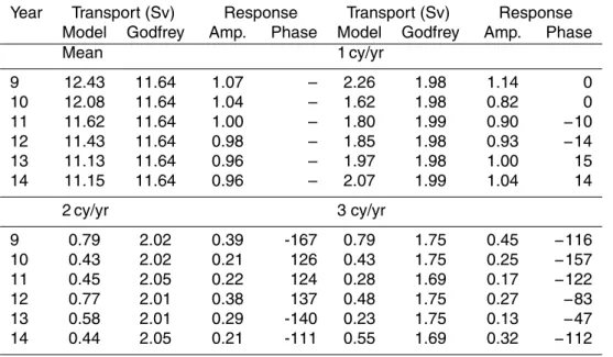
Printer-friendly Version Interactive Discussion Table 3. The mean value of the Indonesian Throughflow in the model, when forced by monthly

climatological winds, and its amplitude at one, two and three cycles per year compared with the value predicted by Godfrey’s Island Rule, during years nine to thirteen of the model run. Also shown is the ratio of the two values and the number of degrees that the model transport delays the wind contribution to the Godfrey integral. Small differences in the Godfrey term arise because the model data is archived on different days each year.

Year Transport (Sv) Response Transport (Sv) Response

Model Godfrey Amp. Phase Model Godfrey Amp. Phase

Mean 1 cy/yr 9 12.43 11.64 1.07 – 2.26 1.98 1.14 0 10 12.08 11.64 1.04 – 1.62 1.98 0.82 0 11 11.62 11.64 1.00 – 1.80 1.99 0.90 −10 12 11.43 11.64 0.98 – 1.85 1.98 0.93 ₋₁₄ 13 11.13 11.64 0.96 – 1.97 1.98 1.00 15 14 11.15 11.64 0.96 – 2.07 1.99 1.04 14 2 cy/yr 3 cy/yr 9 0.79 2.02 0.39 -167 0.79 1.75 0.45 ₋₁₁₆ 10 0.43 2.02 0.21 126 0.43 1.75 0.25 ₋₁₅₇ 11 0.45 2.05 0.22 124 0.28 1.69 0.17 ₋₁₂₂ 12 0.77 2.01 0.38 137 0.48 1.75 0.27 ₋₈₃ 13 0.58 2.01 0.29 -140 0.23 1.75 0.13 ₋₄₇ 14 0.44 2.05 0.21 -111 0.55 1.69 0.32 ₋₁₁₂ 354

(32)

OSD

Full Screen / Esc

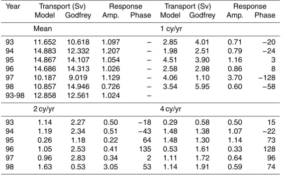
Printer-friendly Version Interactive Discussion Table 4. The mean value of the Indonesian Throughflow in the model, when forced by ECMWF

analysed six-hourly winds, and its amplitude at one, two and three cycles per year compared with the value predicted by Godfrey’s Island Rule, during model years 1993 to 1998. Also shown is the response, the ratio of the two values and the number of degrees that the model transport delays the wind contribution to the Godfrey integral.

Year Transport (Sv) Response Transport (Sv) Response

Model Godfrey Amp. Phase Model Godfrey Amp. Phase

Mean 1 cy/yr 93 11.652 10.618 1.097 – 2.85 4.01 0.71 ₋₂₀ 94 14.883 12.332 1.207 – 1.98 2.51 0.79 ₋₂₄ 95 14.867 14.107 1.054 – 4.51 3.90 1.16 3 96 14.686 14.313 1.026 – 2.58 2.98 0.86 8 97 10.187 9.019 1.129 – 4.06 1.10 3.70 ₋₁₂₈ 98 10.857 14.946 0.726 – 3.54 5.95 0.60 −58 93-98 12.858 12.561 1.024 – 2 cy/yr 4 cy/yr 93 1.14 2.27 0.50 −18 0.29 0.58 0.50 15 94 1.19 2.34 0.51 −43 1.48 1.38 1.07 −22 95 0.26 1.18 0.22 64 1.48 1.30 1.14 73 96 1.05 2.53 0.41 135 0.53 1.61 0.33 128 97 0.96 2.83 0.34 2 1.11 1.72 0.64 96 98 1.63 0.53 3.05 53 1.14 1.91 0.59 74 355