Elastic bending of Variable Curvature Mirrors: validation of a simplified analytical method

HAL Id: hal-02263700

https://hal.archives-ouvertes.fr/hal-02263700

Submitted on 5 Aug 2019

HAL is a multi-disciplinary open access

archive for the deposit and dissemination of

sci-entific research documents, whether they are

pub-lished or not. The documents may come from

teaching and research institutions in France or

abroad, or from public or private research centers.

L’archive ouverte pluridisciplinaire HAL, est

destinée au dépôt et à la diffusion de documents

scientifiques de niveau recherche, publiés ou non,

émanant des établissements d’enseignement et de

recherche français ou étrangers, des laboratoires

publics ou privés.

Elastic bending of Variable Curvature Mirrors:

validation of a simplified analytical method

Xiaopeng Xie, Hui Zhao, Emmanuel Hugot, Liang Xu, Sabri Lemared,

Meiying Liu, Xuewu Fan, Chuang Li

To cite this version:

Xiaopeng Xie, Hui Zhao, Emmanuel Hugot, Liang Xu, Sabri Lemared, et al.. Elastic bending of

Variable Curvature Mirrors: validation of a simplified analytical method. Applied optics, Optical

Society of America, 2019. �hal-02263700�

Elastic bending of Variable Curvature Mirrors:

validation of a simplified analytical method

X

X

,

H

Z

,

E

H

,

L

X

,

S

L

,

M

L

,

X

F

,

C

L

1_{Space Optics Lab, Xi’an Institute of Optics and Precision Mechanics, Chinese Academy of Science, 17}

Xinxi Road, Xi’an, 710119, China

2_{University of Chinese Academy of Science, 19 Yuquan Road, Beijing, 100049, China}

3_{Aix Marseille University, CNRS, LAM, 38 Rue Frédéric Joliot-Curie, Marseille, 13388, France}

*zhaohui@opt.ac.cn

Abstract: This work explores the variable curvature mirror’s (VCM) elastic bending rules

through modeling it as a thin elastic plate with an exponential thickness distribution actuated with a uniform pressure under simply supported boundary conditions. By using the small-parameter method, the general analytical expression of a plate’s deflection is worked out. The results calculated by the analytical solution are compared to the finite element analysis of a VCM model with the same specific parameters. We demonstrate that the two have a good correlation with the one the other. This analytical solution is an effective way to predict a VCM’s deflection.

© 2018 Optical Society of America

1. Introduction

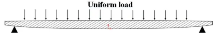
Variable curvature mirror (VCM) is an advanced active optics component whose radius of curvature can be adjusted by an external force to satisfy the need of zoom imaging [1-6], thermal lens compensation [7-10]. These components are used on interferometric telescopes for pupil size stabilization upstream the beams recombination [11-13]. The work published in the literature usually considers a VCM with a uniform or variable thickness distribution and is actuated by either a uniform load, a central force or an annular force [14-17]. The deflection of VCM is an important issue to solve in estimating the process of actuation. Elasticity theory is the most commonly used to estimate the deflection of a VCM. Considering a VCM with uniform thickness distribution, the analytical expression of the deflection under uniform load or annular force is relatively simple [18, 19]. But for VCMs with variable thickness, the solution given by the elasticity theory is in the form of series [18]. In order to analyze the VCMs deflection in that case and obtain a detailed value of the optical surface deflection, we develop in this paper a simplified form of solution by introducing the small-parameter method in the solving process [20]. According to the theory of plates and shells [18], the curvature variation process could be physically modeled as a thin circular plate’s deformation caused by uniform load which has variable thickness and under the simply supported boundary condition, as Fig. 1 displays.

Fig. 1. Physical model of simply supported elastic thin plate with variable thickness

While the thin circular plate is under the simply supported boundary condition with uniform load, the stress condition and the moment equilibrium of the plate is shown in Fig. 2 as follows [20].

0

dr

Q

qdr

_h

r

r

0

r

a

d

b

_c

z

Fig. 2. Stress analysis of physical model of simply supported elastic thin plate’s cross section

The corresponding moment equilibrium equation is, 𝑀𝑟+

𝑑𝑀𝑟

𝑑𝑟 𝑟 − 𝑀𝑡+ 𝑄𝑟 = 0 (1)

With 𝑟 representing the radial coordinate, 𝑑𝑟 is the infinitesimal of 𝑟 , 𝑀𝑟 is the radial

bending moment per unit length, 𝑀𝑡 is the tangential bending moment per unit length and 𝑄 is

the shearing force per unit length. The equations of 𝑀𝑟, 𝑀𝑡, 𝑄 are:

𝑀𝑟= −𝐷 ( 𝑑2_𝑤 𝑑𝑟2+ 𝜇 𝑟 𝑑𝑤 𝑑𝑟) (2) 𝑀𝑡= −D ( 1 𝑟 𝑑𝑤 𝑑𝑟 + 𝜇 𝑑2𝑤 𝑑𝑟2) (3) 𝑄 = 1 2𝜋𝑟∫ 𝑞2𝜋𝑟𝑑𝑟 𝑟 0 (4)

With w as the vertical deflection, 𝐷 = 𝐸ℎ3

12(1−𝜇2) the rigidity of the plate, ℎ the thickness

distribution, 𝜇 the Poisson’s ratio, 𝑞 the load per unit area. By using Eq. (2), (3) and (4) into Eq. (1), we obtain Eq. (5): 𝐷 𝑑 𝑑𝑟 1 𝑟 𝑑 𝑑𝑟(𝑟 𝑑𝑤 𝑑𝑟) + 𝑑𝐷 𝑑𝑟( 𝑑2𝑤 𝑑𝑟2+ 𝜇 𝑟 𝑑𝑤 𝑑𝑟) = 1 𝑟∫ 𝑞𝑟𝑑𝑟 𝑟 0 (5)

As the load is uniform, so Eq. (5) can also be displayed as, 𝐷 𝑑 𝑑𝑟 1 𝑟 𝑑 𝑑𝑟(𝑟 𝑑𝑤 𝑑𝑟) + 𝑑𝐷 𝑑𝑟( 𝑑2𝑤 𝑑𝑟2 + 𝜇 𝑟 𝑑𝑤 𝑑𝑟) = 1 2𝑞𝑟 (6)

Eq. (6) represents the universal form of thin elastic plate under uniform load. When the thickness distribution h changes along with r, the rigidity of the plate also change along with r. In this paper, the thickness distribution of the plate is expressed into the form of ℎ = ℎ0𝑒 −𝛽 6( 𝑟 𝑎) 2

[18]. ℎ0 is the central thickness, a the radius, and different values of β represent

different thickness distribution modes. To solve the deflection w of the plate, first we introduce the following substitutions:

𝑥 = (𝑟/𝑎)2, 𝑦 =𝑤

ℎ0, 𝑄 =

3𝑎4(1−𝜇2) 4𝐸ℎ₀4 𝑞 (7)

By combining Eq. (7) into Eq. (6) we obtain

𝑑2 𝑑𝑥2𝑥 𝑑𝑦 𝑑𝑥− 𝛽 4[2𝑥 𝑑2𝑦 𝑑𝑥2+ (1 + 𝜇) 𝑑𝑦 𝑑𝑥] = 𝑄𝑒 𝛽𝑥 2 ₍₈₎

In the case of a plate which is simply supported along the edge, the boundary condition is: (𝑤)𝑥=1= 0, (𝑀𝑟)𝑥=1= 0 (9)

Eq. (9) can be expressed by 𝑦, 𝑥 as Eq. (10) in the following step, by solving the differential equation to get the corresponding deflection results w of plate.

{ 𝑦 = 0 2𝑑2𝑦 𝑑𝑥2+ (1 + 𝜇) 𝑑𝑦 𝑑𝑥= 0 𝑓𝑜𝑟 𝑥 = 1 (10)

To solve Eq. (8), we chose the small parameter method to work it out [20]. Firstly, we set 𝜀 =𝛽

6, and the y is developed by power series for 𝜀 as in Eq.(11),

𝑦 = 𝑦0(𝑥) + 𝑦1(𝑥)𝜀 + 𝑦2(𝑥)𝜀2+ 𝑦3(𝑥)𝜀3+ 𝑦4(𝑥)𝜀4+. .. (11)

𝑦0, 𝑦1, 𝑦2… are functions for x. Also, the right part of the equation, 𝑒

𝛽𝑥

2 is developed by power series in 𝜀’s order,

𝑒𝛽𝑥2 = 𝑒3𝜀𝑥= 1 + 3𝑥𝜀 +9 2!𝑥 2_𝜀2₊27 3!𝑥 3_𝜀3₊81 4!𝑥 4_𝜀4_{+ ⋯ (12)}

Secondly, by solving the differential equations corresponding to the order of 𝜀, we have the analytical expression of 𝑦0, 𝑦1, 𝑦2, 𝑦3, 𝑦4. We present these five exact solutions in Eq.(15),

Eq.(18), Eq.(21), Eq.(24) and Eq.(27).

0) For 𝑦0, the zero-order equation and the boundary conditions are, 𝑑2 𝑑𝑥2𝑥 𝑑𝑦0 𝑑𝑥 = 𝑄 (13) 𝑦0(1) = 0, 2 𝑑2𝑦0(1) 𝑑𝑥2 + (1 + 𝜇) 𝑑𝑦0(1) 𝑑𝑥 = 0 (14)

The solution is,

𝑦0= 𝑄 4[𝑥 2₋2(3+𝜇) (1+𝜇)𝑥 + (5+𝜇) (1+𝜇)] (15)

1) For 𝑦1, the first-order equation and the boundary conditions are, 𝑑2 𝑑𝑥2𝑥 𝑑𝑦1 𝑑𝑥 = 3 [𝑥 𝑑2𝑦0 𝑑𝑥2 + 1 2(1 + 𝜇) 𝑑𝑦0 𝑑𝑥 + 𝑄𝑥] (16) 𝑦1(1) = 0, 2 𝑑2𝑦1(1) 𝑑𝑥2 + (1 + 𝜇) 𝑑𝑦1(1) 𝑑𝑥 = 0 (17)

The solution is, 𝑦1 = 𝑄 48[2(7 + 𝜇)𝑥 3_{− 9(3 + 𝜇)𝑥}2₊12(−4+3𝜇+𝜇2) (1+𝜇) 𝑥 + (61−16𝜇−5𝜇2) (1+𝜇) ] (18)

2) For 𝑦2, the second-order equation and the boundary conditions are, 𝑑2 𝑑𝑥2𝑥 𝑑𝑦2 𝑑𝑥 = 3 [𝑥 𝑑2𝑦1 𝑑𝑥2 + 1 2(1 + 𝜇) 𝑑𝑦1 𝑑𝑥 + 3 2𝑄𝑥 2_{] (19)} 𝑦2(1) = 0, 2 𝑑2_𝑦 2(1) 𝑑𝑥2 + (1 + 𝜇) 𝑑𝑦₂(1) 𝑑𝑥 = 0 (20)

The solution is, 𝑦2= 𝑄 256[(59 + 12𝜇 + 𝜇 2_)𝑥4_{− 8(9 + 6𝜇 + 𝜇}2_)𝑥3_{+ 24(−4 + 3𝜇 + 𝜇}2_)𝑥2₊ 4(1+31𝜇−25𝜇2−7𝜇3) (1+𝜇) 𝑥 + (105−51𝜇+47𝜇2+11𝜇3) (1+𝜇) ] (21)

3) For 𝑦3, the third-order equation and the boundary conditions are, 𝑑2 𝑑𝑥2𝑥 𝑑𝑦3 𝑑𝑥 = 3 [𝑥 𝑑2𝑦2 𝑑𝑥2 + 1 2(1 + 𝜇) 𝑑𝑦2 𝑑𝑥 + 3 2𝑄𝑥 3_{] (22)} 𝑦2(1) = 0, 2 𝑑2_𝑦 2(1) 𝑑𝑥2 + (1 + 𝜇) 𝑑𝑦₂(1) 𝑑𝑥 = 0 (23)

The solution is, 𝑦3= 𝑄 25600[6(605 + 143𝜇 + 19𝑢 2_{+ 𝜇}3_)𝑥5_{− 75(45 + 39𝜇 + 11𝜇}2_{+ 𝜇}3_)𝑥4₊ 400(−12 + 5𝜇 + 6𝜇2_{+ 𝜇}3_)𝑥3_{+ 150(1 + 31𝜇 − 25𝜇}2_{− 7𝜇}3_)𝑥2₊ 30(75−172𝜇−114𝜇2+172𝜇3+39𝜇4) (1+𝜇) 𝑥 + (2145+4972𝜇+898𝜇2−2380𝜇3−451𝜇4) (1+𝜇) ] (24)

4) For 𝑦4, the fourth-order equation and the boundary conditions are, 𝑑2 𝑑𝑥2𝑥 𝑑𝑦4 𝑑𝑥 = 3 [𝑥 𝑑2𝑦3 𝑑𝑥2 + 1 2(1 + 𝜇) 𝑑𝑦3 𝑑𝑥 + 9 8𝑄𝑥 4_{] (25)}

𝑦4(1) = 0, 2 𝑑2𝑦4(1)

𝑑𝑥2 + (1 + 𝜇)

𝑑𝑦4(1)

𝑑𝑥 = 0 (26)

The solution is, 𝑦4= 𝑄 102400[(7365 + 1892𝜇 + 314𝜇 2_{+ 28𝑢}3_{+ 𝜇}4_)𝑥6_{− 18(315 + 318𝜇 + 116𝜇}2₊ 18𝜇3_{+ 𝜇}4_)𝑥5_{+ 150(−60 + 13𝜇 + 35𝜇}2_{+ 11𝜇}3_{+ 𝜇}4_)𝑥4_{+ 100(3 + 94𝜇 − 44𝜇}2₋ 46𝜇3_{− 7𝜇}4_)𝑥3_{+ 45(75 − 172𝜇 − 114𝜇}2_{+ 172𝜇}3_{+ 39𝜇}4_)𝑥2₋ 18(205+219𝜇−1098𝜇2−6𝜇3+573𝜇4+107𝜇5) (1+𝜇) 𝑥 + 2(3660+3897𝜇−6744𝜇2+726𝜇3+2316𝜇4+369𝜇5) (1+𝜇) ] (27)

According to the reference [20], with the increase of the order of the y, the influence of it decreases. So the influence of solution y to the deformation of plate which exponent is higher than 4th can be neglected. Comparing to the results we present in this paper, Ref. [18] gives a quite complicated solution in the form of series, shown in Eq. (28).

𝜑 = 𝑝 [𝐶𝜑1− 𝑟𝑒 𝛽 2 ( 𝑟 𝑎) 2 𝑎(3−𝜇)𝛽] (28) 𝜑1= 𝑎1[ r 𝑎+ ∑ 𝛽𝑛(1+𝜇)(3+𝜇)⋯(2𝑛−1+𝜇) 2∙4∙4∙6∙6⋯2𝑛∙2𝑛(2𝑛+2) ∞ 𝑛=1 ( 𝑟 𝑎) 2𝑛+1_{] (29)}

C is a constant which is determined from the boundary condition of the thin elastic plate,

𝑎1is an arbitrary constant, p is pressure, which is 𝑝 =

6(1−𝜇2_)𝑎3_𝑞

𝐸ℎ₀3 .

Also, it gives the coefficient α which is used to estimate the central deflection as a function of β. The original equation develops like Eq. (30).

𝑤𝑚𝑎𝑥 = 𝛼𝑎𝑝 = 𝛼

6(1−𝜇2)𝑎4𝑞 𝐸ℎ₀3 (30)

And the central deflection (x=0) which is calculated by us in Eq. (11) can be developed like this, 𝑦(0) = 𝑄 [1 4 (5+𝜇) (1+𝜇)+ 1 48 (61−16𝜇−5𝜇2) (1+𝜇) 𝜀 + 1 256 (105−51𝜇+47𝜇2+11𝜇3) (1+𝜇) 𝜀 2₊ 1 25600 (2145+4972𝜇+898𝜇2−2380𝜇3−451𝜇4) (1+𝜇) 𝜀 3₊ 1 102400 2(3660+3897𝜇−6744𝜇2_+726𝜇3_+2316𝜇4_+369𝜇5₎ (1+𝜇) 𝜀 4 _{] (31)}

The next step consists in transforming Eq. (31) into a form similar to Eq. (30) to work out the value of α and compare the two α’s values. That will allow to verify the accuracy of the small parameter method.

Table 2. Comparison of α values between Ref. [18] and this paper corresponding to different thicknesses of the plate β α 4 3 2 1 0 -1 -2 -3 -4 Ref. [18] 0.2233 0.1944 0.1692 0.1471 0.1273 0.1098 0.0937 0.0791 0.06605 This paper 0.2232 0.1943 0.1691 0.1470 0.1274 0.1097 0.0937 0.0792 0.06620

From the table, we can see that up to the 4th _{order the two α’s result value is almost the same.}

It means that the solution solved by small parameter method can reach a quite high accuracy.

3. Finite element analysis (FEA)

To verify the mathematical solution’s effectiveness in predicting the deflection of mirror under different pressure, we compare the Finite Element Analysis (FEA) results of designed VCM model to the value calculated by Eq. (11). For this verification, we choose 𝛽 = 3 as the lower surface’s thickness distribution coefficient, then the thickness expression is: ℎ = ℎ0𝑒−

𝑥 2_{. First,}

on the other side shown in Fig. 1 and extract the deformation value of it along the radial direction. Then, we compare it to the value calculate by our analytical solution. In real application, as the mirror is actuated by air pressure, the elastic thin plate needs to be designed as a closed cavity, so collar is added into the mirror design like shown in Fig. 3. Considering the application need, the existing designed mirror’s parameters are the following: diameter 2𝑎 = 134.5mm, central thickness ℎ0= 8.5mm, material is ultralumin (E=72GPa, μ=0.33),

and thin collar’s thickness 𝑐 = 0.62mm. So the second compare is the real designed mirror model and the analytical solution. Therefore, we build the VCM model shown in Fig. 3 in Solidworks using referred parameters and import it to ANSYS to do the FEA.

Fig. 3. Structure design of pressurization actuation VCM having variable thickness

Fig. 4. Structure of 1/2 upper mirror’s cross section

4. Comparing of FEA and analytical model

During the FEA process, we set the elastic thin plate under simply supported edge condition and apply 0.1MPa at its surface. Then we get the deflection curve along its radius. Here is the comparison between the elastic thin plate’s FEA results to the analytical solution, shown in Fig.5. From Fig.5, the two curves’ difference is very small and the deformations present good consistency. By doing subtraction between the two curves’ values, we extract the difference between them, shown in Fig.6. The maximum difference is 0.72μm and decrease to nearly 0 on the edge.

Thickness distribution

Thin collar Mirror’s base

Fig. 5 Elastic thin plate’s FEA and analytical deflection curves at 0.1MPa

Fig. 6 The subtraction of the normalized deflection, analytical and FEA, has the shape of a spherical aberration.

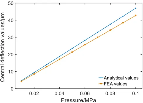
Then, we compare the FEA deflection values of designed VCM and the analytical solution’s deflection values under 0.01MPa to 0.1MPa which is shown in Fig.7. From the Fig.7, we can see mirror’s deflection values decrease with the introducing of thin collar which consume part

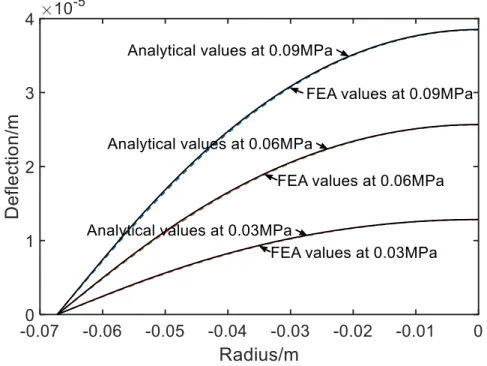
of the pressure. In addition, the deflection values of FEA and analytical solution along the radius direction under 0.03MPa, 0.06MPa and 0.09MPa are abstracted to plot the Fig. 8.

Fig. 7 Comparison of central deflection values given by Eq. (16) and Finite element analysis

Fig. 8 Comparison of surface deformation along radius direction between values given by Eq.(13) and obtained through FEA

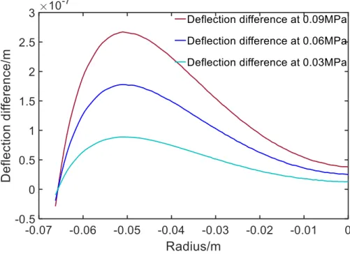
From Fig. 7 and Fig. 8, we can see that all the deflection curves obtained by the two methods have a good consistency, although the two values are not exactly the same. As the basic theory’s

ideal boundary condition is hard to be achieved under air pressure actuation, the thin collar’s existence adds semi-clamps effect to the mirror’s boundary condition [11]. And by Ref.[11], the values of the two methods are further fitting by using 𝑃𝑐= 𝑃0(1 + 𝑐/𝑡)3. 𝑃0, the theoretical

pressure needed to achieve a given curvature in simply supported boundary condition, 𝑃𝑐, the

pressure needed in case has a thin collar with a semi-clamped effect. 𝑐, 𝑡 represent the thin collar’s thickness and the central thickness of the VCM respectively. As one can see from the comparison in Fig.7, the theoretical central deformation result is higher than the FEA result under same pressure value, so we use this rule to calculate the theoretical value that can produce the same central deflection with FEA. In Ref.[11], the equation is suitable for mirror’s collar thickness from 0 to 50μm, so we can adjust the equation by change it to 𝑃𝑐 = 𝑃0(1 + 𝑐/𝑡)𝑚. As

the analytical value is easier to calculate by the software, so we think about the condition in verse. Assuming the mirror can achieve the same deflection, and the FEA pressure is 0.09MPa, the theoretical pressure that is needed to achieve the same is less than 0.09MPa. We set it as 𝑃0= 𝑃𝑐/(1 + 𝑐/𝑡)𝑚, after calculation, when 𝑚 = 1.33, equally 𝑃0= 0.082𝑀𝑃𝑎, the FEA and

analytical results are nearly the same shown in Fig.9, especially the central part. Fig.10 shows the deflection difference curve of each two curves at 0.09MPa, 0.06MPa, 0.03MPa pressure values and the corresponding RMS of the deflection difference are 168nm, 112nm and 56.2nm. Also Fig.11 shows the variation tendency of the deflection difference’s RMS values under the pressure mentioned above. Comparing the two pressure values, about 9% of the pressure is consumed by semi-clamps effect under this collar thickness condition.

Fig. 10 Deflection difference of the each two curves in Fig.9 at 0.09MPa, 0.06MPa, 0.03MPa

Fig. 11 Variation tendency of the deflection difference’ RMS at 0.03MPa, .06MPa, 0.09MPa

5. Conclusion

To conclude, in this paper, we developed the analytical solution of a thin elastic plate with variable thickness distribution under simply supported boundary condition by using the small parameter method. It is a quite simple solution easy to be analyzed. Through calculating the

central deflection coefficient α, the results get by small parameter method is very accurate for the analytical results. The further verification is done between analytical solution and FEA results through software analysis. The elastic thin plate’s analytical solution and FEA results and the designed mirror’s deflection calculated by mathematical method and FEA are consistent. By further fitting both of them, there is almost no difference between the deformation curves especially in the central area of the mirror, approximately 9% of pressure is consumed by semi-clamp effect. So the analytical results can have a good predict to the FEA’s deformation results. The prototype of VCM is under study to obtain the practical data during the actuation process to compare to it. Additionally, the optimization of the VCM’s parameter is under study to obtain a better central deflection and surface optical quality.

Funding

West Light Foundation of Chinese Academy of Science(XAB2015A09); Youth Science and Technology Star of Shaanxi Provence (2016KJXX-08); National High Technology Research and Development Plan; China Scholarship Council; European Research Council ICARUS Program (H2020-ERC-STG-2015/678777).

References

1. K. SEIDL, K. RICHTER and J. KNOBBE, “Wide field-of-view all-reflective objectives designed for multispectral image acquisition in photogrammetric applications,” Proc of SPIE 8172(817210), (2011). 2. K. SEIDL, J. KNOBBE and H. GRUGER, “Design of an all-reflective unobscured optical-power zooming

objective,” Appl. Opt.48(21),4097-4107 (2009)..

3. H. L. Yu, L. L. YEN and D. J. S. Guo. “Optical zoom module based on two deformable mirrors for mobile device application,” Appl. Opt.51(11), 1804-1810 (2012).

4. H. Zhao, X. W. Fan and G. Y. Zou, “Prototype design of an all-reflective non-coaxial optical zooming system for space camera application without moving elements based on deformable mirror,” Proc of SPIE 8557(855713), (2012).

5. B. E. Bagwell, D. V. Wick and W. D. Cowan, “Active zoom imaging for operationally responsive space,” Proc of SPIE 6467(64670D), (2007).

6. D. V. Wick, T. Y. Martinez and D. M. Payne, “Active optical zoom system,”Proc of SPIE 5798,151-157,(2005). 7. U. J. Greiner and H. H. Klingenberg. “Thermal lens correction of a diode-pumped Nd:YAG laser of high TEM00

power by an adjustable-curvature mirror,” Opt. Lett. 19(16), 1207-1209, (1994).

8. V. V. Apollonov, G. V. Vdovin, L. M. Ostrovskaya and Sov. J. “Active correction of a thermal lens in a solid-state laser. I. Metal mirror with a controlled curvature of the central region of the reflecting surface,” Quant. Electr. 21(1), 116-117, (1991).

9. J. Schwarz, M. Ramsey and D. Headley, “Thermal lens compensation by convex deformation of a flat mirror with variable annular force,” Appl. Phy. B82, 275-281 (2006).

10. Z. Q. Feng, L. Bai and Z. B. Zhang, “Thermal deformation compensation of high-energy laser mirrors,” Opt. and Prec. Eng. 18(8), 1781-1787, (2010).

11. M. Ferrari and F. Derie, “Variable curvature mirrors for the VLTI,” Proc. of SPIE 3350(830), (1998). 12. Z. Challita, E. Hugot and F. Madec,” Active Optics: Variable Curvature Mirrors for ELT laser guide star refocusing systems,”

Proc of SPIE 8172(81721A), (2011).

13. E. Hugot, M. Ferrari and G. R. Lemaitre, “Active optics for high-dynamic variable curvature mirrors,” Opt. Lett. 34(19), 3009-3011, (2009).

14. G. R. Lemaitre, Astronomical optics and elasticity theory, Springer, 2009.

15. E. L. J. Matthew and C. W. Christopher, “Large-aperture active optical carbon fiber reinforced polymer mirror,” Proc. of SPIE 8725(87250W), (2013)

16. X. P. Xie, H. Zhao, and Ch. Li, “Annular force based on variable curvature mirror technique,” Acta. Phot. Sini. 45(8),0822001-1-0822001-10, (2016)

17. H. Zhao, X. P. Xie and J. X. Wei, “Annular force based variable curvature mirror aiming to realize non-moving element optical zooming,” Proc. of SPIE 9678(967807), (2015).

18. S. P. TIMOSHENKO and S. W. KRIEGER. Theory of plates and shells, the 2nd edition, Singapore: McGraw-Hill Book Company, 1959.

19. C. Y. Warren, G. B. Richard, Roark’s Formulas for stress and strain, the seventh edition, 2002. 20. K. Y. Yeh, “Bending of a thin elastic plate of variable thickness,” Acta. Phys. Sin. 113 (1955).