HAL Id: hal-01084731
https://hal.archives-ouvertes.fr/hal-01084731
Submitted on 19 Nov 2014HAL is a multi-disciplinary open access archive for the deposit and dissemination of sci-entific research documents, whether they are pub-lished or not. The documents may come from teaching and research institutions in France or abroad, or from public or private research centers.
L’archive ouverte pluridisciplinaire HAL, est destinée au dépôt et à la diffusion de documents scientifiques de niveau recherche, publiés ou non, émanant des établissements d’enseignement et de recherche français ou étrangers, des laboratoires publics ou privés.
constrained system
Matthieu Labousse, Stéphane Perrard, Yves Couder, Emmanuel Fort
To cite this version:
Matthieu Labousse, Stéphane Perrard, Yves Couder, Emmanuel Fort. Build-up of macroscopic eigen-states in a memory-based constrained system. New Journal of Physics, Institute of Physics: Open Access Journals, 2014, 16, pp.113027. �10.1088/1367-2630/16/11/113027�. �hal-01084731�
This content has been downloaded from IOPscience. Please scroll down to see the full text.
Download details:
This content was downloaded by: labousse IP Address: 193.54.87.192
This content was downloaded on 14/11/2014 at 14:22
Please note that terms and conditions apply.
Build-up of macroscopic eigenstates in a memory-based constrained system
View the table of contents for this issue, or go to the journal homepage for more 2014 New J. Phys. 16 113027
based constrained system
M Labousse1, S Perrard2, Y Couder2and E Fort3
1Institut Langevin, ESPCI Paristech, CNRS, Pierre and Marie Curie University, 1 rue Jussieu,
75005, Paris, France
2
Laboratoire Matière et Systèmes Complexes , Université Paris Diderot 10 rue Alice Domon et Léonie Duquet, 75005 Paris, France
3
Institut Langevin, ESPCI Paristech, CNRS, PSL Research University, 1 rue Jussieu, 75005, Paris, France
E-mail:[email protected],[email protected],[email protected]
Received 14 July 2014, revised 3 September 2014 Accepted for publication 19 September 2014 Published 11 November 2014
New Journal of Physics 16 (2014) 113027
doi:10.1088/1367-2630/16/11/113027 Abstract
A bouncing drop and its associated accompanying wave forms a walker. Based on previous works, we show in this article that it is possible to formulate a simple theoretical framework for the walker dynamics. It relies on a time scale decomposition corresponding to the effects successively generated when the memory effects increase. While the short time scale effect is simply responsible for the walkerʼs propulsion, the intermediate scale generates spontaneously pivotal structures endowed with angular momentum. At an even larger memory scale, if the walker is spatially confined, the pivots become the building blocks of a self-organization into a global structure. This new theoretical framework is applied in the presence of an external harmonic potential, and reveals the underlying mechanisms leading to the emergence of the macroscopic spatial organization reported by Perrard et al (2014 Nature Commun. 5 3219).
Keywords: memory-based dynamics, Wave self-organization, nonlinear dynamics
Content from this work may be used under the terms of theCreative Commons Attribution 3.0 licence. Any further distribution of this work must maintain attribution to the author(s) and the title of the work, journal citation and DOI.
1. Introduction
Complex systems often require building several hierarching levels of description. This raises fundamental questions in high-dimensional systems about the relevant amount of information needed to characterize them [2–4]. Here, we investigate the case of a strongly nonlinear dynamics in which its apparent complexity can be tremendously reduced, giving way to the surprising quantification of its observables.
An experimental situation has revealed that a walker [5], this macroscopic association of a bouncing drop and its accompanying wave, exhibits a dynamics sufficiently complex to reproduce at an unusual scale, a quantum-like effect such as diffraction through submarines slits [6], tunnelling [7], Zeeman-like splitting [8], wave-like statistics in cavities [9], or else a Landau level analogue [10–12]. Perrard et al [1] investigated the case where the system, a droplet set on a vertically- vibrated bath and self-propelled by its accompanying wave, is subjected to a two-dimensional (2D) harmonic central potential of natural frequency ω π2 . They singled out elementary paths on which the full dynamics can be decomposed. In particular, they showed that the phase space of the dynamics can be projected on a state diagram (n,m). The integer n is associated with the time-average orbit extension and m the quantized mean angular momentum, satisfyingm ∈ −{ n, − +n 2, …, n − 2, } reminiscent of the quantum selection rules. In then
current paper, we investigate the mechanism responsible for the emergence of these macroscopic eigenstates.
As in the previous reported experiments, we consider a millimetric drop of silicon oil bouncing on a bath oscillating vertically at a frequency f0 = 80 Hz, with an acceleration
γ = γm cos (2πf t0 ). The coalescence is prevented by the permanent presence of a thinfilm of air between the drop and the bath [13–16]. In addition, above a critical Faraday acceleration threshold γF, the surface is unstable at a frequency f 20 , and standing waves appear spontaneously as initially observed by Faraday [17] and further studied in [18–20] (see the review [21] and references therein). We restrain our study to the case with period doubling at an acceleration amplitude γm slightly below the Faraday acceleration threshold, typically
γF (γF − γm) ∼ 0.98. In this situation, the drop excites parametrically the surface wave, each impact generating a Bessel-like mode centred at the impact point [22,23]. The surface height h derives from the linear superposition of the elementary contributions of the previous impacts. Each contribution relaxes to the equilibrium over a typical time decay; henceforth the memory time τ = MTF. This memory parameter M indicates the relevant number of secondary sources
contributing to the surfacefield.M∼ γF (γF− γm)is tuned by changing the driving acceleration amplitude. Impacts that occurred more than a few M Faraday periods in the past are negligible. Above a critical memory parameter Mc∼ 3, the vertical bouncing state is unstable to a horizontal perturbation . The drop lands on an inclined surface and acquires an increment of horizontal momentum proportional to the local slope [10, 23, 24], which initiates a horizontal motion at typical speed ∼10 mm s−1.
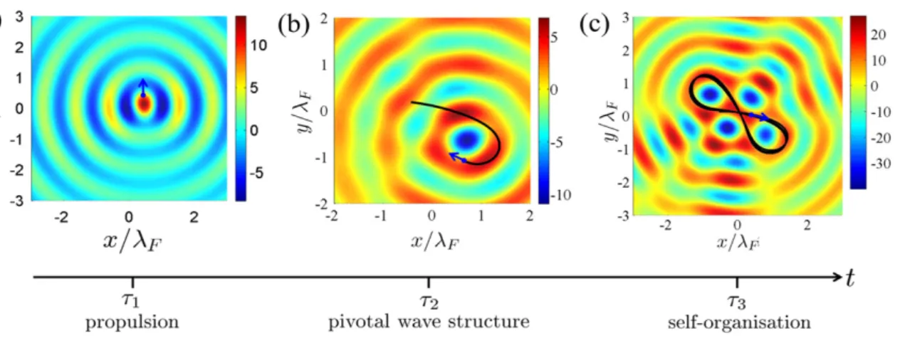
Figure1represents typical examples of the wavefield and the associated horizontal walker dynamics as the memory increases. For short memory parameter M (seefigure1(a)), the surface field mainly propels the droplet forward at a constant speed. This regime defines the short time scale τ ∼ T1 F and the eponymous dynamics. For intermediate memory parameter M (see
figure 1(b)), an increasing number of secondary sources can interfere, and semi-local surface field structures can arise. The walker can turn around these structures and reinforce them. We unambiguously call these characteristic wave structures, pivotal wave structures. This
phenomenon acts on a typical time scale τ2 ≫τ1 and defines the intermediate time scale
dynamics. As the memory is much larger (seefigure1(c)), several reminiscent pivotalfields can coexist, and a global coherent structure emerges from an apparently complex path. It corresponds to a well-defined organization of these pivotal wave structures. This organization acts on a third time scale τ3≫ τ2 ≫τ1and defines the long time scale dynamics. It indicates a
clear separation of time scale, associating with space scale organization of well-defined surface field structures. At long memory, all these time scales interlock, and the effect of each of them can be revealed as the memory parameter increases. The main goal of this paper is to present a theoretical framework in the presence of an attractive potential in the light of this spatio-temporal separation of scales. As it is surprising that this macroscopic wave particle association, when immersed into a harmonic potential, gives rise to a set of attractors with a classical selection rule reminiscent of its quantum counterpart [1], we propose to apply this theoretical framework to explain how such classical attractors emerge.
In the first part, we recall the symmetry properties of the surface field and their consequence on its further time-scale decomposition. In the second part, we formulate the short time dynamics and express it close to the constraint of small speedfluctuations. In the third part, we zoom out a first time, and we add the semi-local wave structure emerging from the pivotal field. The dynamics is described in the Frenet-adapted wave basis and shows that this basis is actually adapted to the translational invariance property of the surfacefield. We describe how the system evolves with preferred radii of curvature. These pivotal structures constitute the basic units of the dynamics. In the last part, we zoom out once again and see how these pivots interact and organize with each other, which defines the long time dynamics. We show that this self organization emerges from a compromise between two a priori incompatible symmetries. The location of the translational-invariant pivotal fields have to account for the rotational-invariant central force.
Figure 1. Typical example of a walker dynamics in a harmonic potential (here
ω π = Hz
( 2 1.32 ) in a natural unit or ω π =( 2 0.0330) in a Faraday period time unit) and the corresponding wavefield as the memory increases. In this specific case the time average speed is 7.9 mm s−1. The wavefields are reconstructed from the simulated paths (Fort numerical model [1]). (a) Local structure: memory M = 9, the wave field propels the drop. (b) Semi local structure: M = 19, some semi local pivotal structures arise. The drop is propelled and guided by a pivotal surface wave field. (c) Global structure: M = 150, the drop is now propelled and guided in a fully coherent structure, corresponding to a well-defined organization of the pivotal surface wave field.
2. The space-time separation of thefield
The theoretical description of the walker dynamics has already been introduced in previous works [5, 10, 15, 22, 24]. The idea of this paper is to use the time scale separation of the dynamics to reduce the complexity of the existing theoretical frameworks. As the drop bounces synchronously with the bath every Faraday period, and the horizontal distance between two impacts is much smaller than the Faraday wavelength, the horizontal dynamics can be approximated by a continuous description [24]
⎡ ⎣ ⎢ ⎤ ⎦ ⎥ γ = − − − t C h E m v v d d [ ] t (1) p t r r ( ) ( )
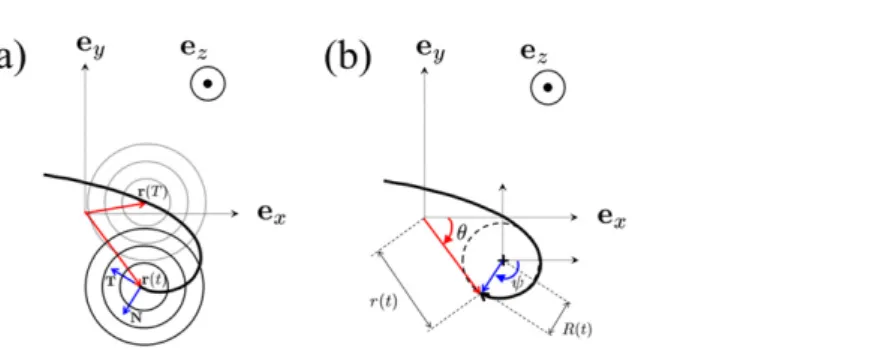
with r the horizontal drop position and v its horizontal speed as sketched in figure 2(a). The length scales and time are normalized by λF 2π (λ = 4.75F mm) and the Faraday period TF (TF = 25 ms). Ep denotes an external attractive potential that will be further specified. The interaction with the surface consists in an apparent friction term -γv and a coupling with the local slope of the surface field −C[h]r( )t , the gradient being taken at the drop position at a
given time. In principle, the coefficients γ and C can be deduced from the benchmarked Fortʼs numerical model [1,6,10] or from the hydrodynamic model of Moláček et al [15,23]. They are used here as free parameters and further chosen to match the experiments. Evaluating thisfield at the instantaneous particle positionr( ) yields [t 10, 24].
∫
= ∥ − ∥ −∞ − − h t T T J t T e r r r ( , ) d ( ( ) ( ) ) (2) t F t T M 0 ( )with J0thefirst order Bessel function, being centred at the point of a past impactr( )T and felt at
t
r( ), the current position of the drop. The origin of different time scales arises intrinsically from the surface term. It is typically the time interval required to generate different hierarchies of coherent wave structures. In paragraph 2.1, we first recall symmetry properties of the surface field h and we use them in paragraph 2.2 to separate the different time scales of the dynamics
Figure 2.(a) Schematics of the dynamics. The origin of referential e( ,x ey)corresponds to the minimum of energy of the attractive potential. The motion defined the tangential and the normal direction so that T N( , ) forms a direct basis. The standing wave-field at a given instant t interferes with the remaining standing wave generated in the past (for all past sources so thatT < t). (b) We define two bases: the polar basis( , ) of originr θ
prescribed by the minimum of energy of the attractive potential and the basis( ,R ψ) of origin at the instantaneous centre of curvature. R denotes the algebraic radius of curvature.
Figure 3.(a) Simulated circular motion (n,m) = (2,−2) at M = 21 ([1], supplementary methods) for ω π =2 0.023 (in Faraday period time unit). The position of the drop is indicated by a blue spot and the whole circular motion by the red circle of radius
λ
≃0.9 F. The circles in black dotted lines correspond to the extrema of the Bessel function of order 0 centred at the origin and plotted in the above sub-figure. The surface field is reconstructed a posteriori, owing to equation (2), and is similar to the experimental one. We can separate the surface field into two terms: an intense part, immediately following and propelling the drop and a coherent part resulting from the interference of the secondary sources. (b) Simulated lemniscate motion (n,m) = (2,0) at M = 21 [1] for ω π =2 0.033 (in Faraday period time unit). The black line indicates the path followed by the drop. The red points denote the loci of the instantaneous centre of curvature. Rcdenotes the centre of the pivotalfield and corresponds to the barycentre of
the damped past sources. (c) and (e) Pivotal structure of a lemniscate. (c) In the blue line, the slice of the wavefield; in the black line, a centred Bessel function of order 0 of negative amplitude. From Rc: the symmetry of the efficiently- contributed path is
roughly rotational-invariant and generates the surface field corresponding to this symmetry at the leading order. (e) We superpose the reconstructed wave field and the path (ω π =2 0.033 (in Faraday period time unit)). The black line qualitatively indicates the part of the path effectively contributing to the wavefield (typically a dimensionless memory curvilinear length ≃VMTF λF). As the drop is turning back to the centre, it
generates a wavefield: a Bessel function of order 0 centred in Rc. (d) and (f) The pivotal
structure of a trefoil (n,m) = (4,2). (d) and (f) are similar to (c) and (e) but for a trefoil (ω π =2 0.016 (in Faraday period time unit)).
2.1. Symmetry properties of the surface field
The dynamics relies on three difference time scales: the propulsion, the semi-local structure, and the global organization. Zooming in on these different dynamical aspects requires developing different tools, particularly in order to describe the surfacefield.
Being a solution of the two dimensional Helmholtz equation, the local value of the surface field can be decomposed into a polar Bessel eigenfunction{ ( ˜, ˜)}f rn θ n∈ = { ( ˜)e )}J rn i ˜nθ n∈, with
a free choice in the centre of decomposition. In this sense, the wavefield revealed translational-invariant properties. The surface field can be indifferently decomposed onto a Frenet-adapted wave basis{fnF( )}t n∈ = { ( ( ))eJ R tn inψ( )t }n∈
⎧ ⎨ ⎪⎪ ⎩ ⎪ ⎪
∫
∑
= = = ψ ∈ −∞ − − − h t t h f t h t h f T T J R T r ( ( ), ) ( ) ( ) d ( ( ))e e (3) n nF n F n F n F t F n in ( )T (t T)Mas well as onto a basis of centre adapted to the external potential
= θ ∈
{
}
∈{
fn ( )t}
J r t( ( ))e n n n t n ext i ( ) ⎧ ⎨ ⎪⎪ ⎩ ⎪ ⎪ ∫
∑
= = = θ ∈ −∞ − − − h t h f t h t h f T T J r T r ( , ) ( ) ( ) d ( ( ))e e (4) n n n n n t F n n T t T M ext ext ext ext i ( ) ( )The different coordinates are indicated in figure 2(b) and correspond to two different polar bases. In equation (3), the Frenet basis R denotes the instantaneous radius of curvature, whileψ indicates the local polar angle having its origin at the instantaneous centre of curvature. In the central polar basis decomposition (equation (4)),( , )r θ indicates the usual polar coordinates, the origin coinciding with the centre of the external potential. Let us briefly mention that in both equations (3) and (4), no imaginary part is effectively added, and the whole expression remains real.
Equations (3) and (4) are mathematically equivalent and simply correspond to two different viewpoints. The decomposition in the Frenet basis (equation (3)) corresponds to a projection of the local value of the wavefield into eigenmodes. This decomposition will be used in section4to express the intermediate time scale dynamics. The decomposition onto a central basis reflects the symmetry of the harmonic potential. We will study in paragraph 5 how the pivotal wave structure builds a long term self-organization.
2.2. Time scale decomposition of the surface field
Distinguishing the different time scales of the dynamics requires separating two physical effects taking place at the surface: the propulsion and the construction of an intermediate/long time coherent surface field structure. To highlight the separation of these two physical effects, the path and the surface field corresponding to the circular attractor (n,m) = (2,2) are shown in figure 3(a). It was obtained from path memory simulations (see [1] supplementary materials). As the memory and the position of each impact are known, the surfacefield can be numerically reconstructed from equation (2). Two distinct parts of the field can be distinguished in
figure3(a), thefirst one, intense, directly following the drop and providing the propulsion, and the second one arising from the constructive interference of the secondary sources left all along the path. This coherent surfacefield structure has a dominant term reflecting the signature of the rotational symmetry of the path, here J0(2πR λF), as emphasized by sub-figure 3(a). The propulsion is short-term acting, while the constructive interference requires a much larger duration to be established. This separation of time scales can be revisited in a theoretical manner, considering the work of Oza etal [11] and M Miskin [25] for a circular path of radius rc of angular speed ωc. The coupling with the local slope of the surface field −C h circle can be theoretically derived, leading to
⎧ ⎨ ⎪ ⎪ ⎩ ⎪ ⎪ ⎛ ⎝ ⎜ ⎞ ⎠ ⎟ ⎛ ⎝ ⎜ ⎞ ⎠ ⎟ ω ω ω ∂ = − − + ∂ = +
(
)
h r J r M h MJ r J r M 1 1 ( ) 1 ( ) (a) ( ) ( ) 1 (b) (5) T c c c N c c circle 02 2 circle 0 1 2where ∂N and ∂T denote the gradients along the normal and tangential direction to the trajectory.
The tangential gradient of thefield (equation (5)(a)) becomes independent of the memory M in the long memory limits. It indicates that the propulsion is a short time effect (further indexed st) . On the contrary, the growth of the normal gradient (equation 5(b)) with the memory M indicates a longer time effect (further indexed lt). The propulsion slightly depends on the memory at the leading order, as it would be a short-acting effect. On the opposite, it takes at least a few memory times to establish the constructive interferences leading to (equation 5(b)). Guided by this idea, it becomes natural to decompose the field for any path into two parts
= +
h Hst Hlt (6)
and dissociate the propulsive contribution Hst from the coherent structure Hlt. The short time effect, being mainly propulsive, admits mainly a tangential component and also imposes
∂NHst ≃ 0, hypothesis (a) (7)
As a corollary, the propulsion being a short term action, we define the long term evolution of thefield so that it does not contribute anymore to the propulsion, i.e.,
∂THlt = 0, hypothesis (b) (8)
These two hypotheses impose two constraints, which, should have consequences on the description of thefield. The Frenet decomposition of the surface wave (equation (3)) prescribes
∑
∑
= + = + ψ ∈ ∈ h( , )r t h f ( )t h f ( )t h J R t( ( )) h J R t( ( ))e . (9) * * F n nF nF F n nF n n t 0 0F 0 0 i ( )Seeking in equation (9), the terms having a zero tangential derivative (hypothesis (b)) yields =
Hlt h f0F 0F( )t . Consequently, we identifyHst = ∑n∈*h fnF nF( )t . Note that hypothesis (b) can be taken as a definition of Hlt. Hst contains all the tangential derivatives and is the only one
responsible for the propulsion. Section 3is devoted to this short time scale dynamics and will express ∂ HT st on its symmetry in speed. But what about hypothesis (a)? As we remain in the
component ∂ HN st [26]. But is it still valid as we get into a longer memory regime? Section 4
deals with the intermediate time scale dynamics and will investigate how this physical hypothesis stands as we go onto a more complex trajectory.
3. Short time scale dynamics: the propulsion
The income of energy to the drop mediated by Hst increases its horizontal momentum.
Nevertheless, as the friction starts acting, the drop loses a part of energy, and a dynamical exchange of its energy between the surface field and the drop occurs. This process defines a steady velocity v0 at which the energy propelling the particle balances its frictional loss of energy. In the regime parameter of interest, this equilibrium speed is a constant of the motion. In the phase space of the dynamics, this constraint defines a manifold in the neighbourhood of which it is convenient to express the dynamics. This constraint on speed contains some of the major non Hamiltonian features of the dynamics in the short memory regime as shown in [26]. Experiments and path-memory simulations of the dynamics in a harmonic potential [1] showed that for a given drop, the mean velocity is a constant of the motion, and the corresponding fluctuations remain small (typically ∼10%). In the tangential direction, the combined effect of friction and propulsion from the surface f v( ) can be expressed as
γ γ
= − − ∂ = − + ∂
( )
C h(
v C H)
f v v T T T st T. (10)
Let us mention that only the short term field Hst contributes in the tangential direction, as ∂THlt = 0. f v( ) is tangential to the trajectory i.e., f v( ) = f( ) . The amplitude of thev T propulsion f v( ) must providev0as afixed point and also is only a function of the amplitude of
the speed i.e.,f v( )= f v( ) . Additionally, f(v), must be odd in v as a complete reverse of theT
instantaneous of the motion should not break any symmetry in the propulsion, i.e., − = −
f ( v) f v( ). It has been shown [26] that at the smallest order of fluctuations, the propulsion should be written as
Γ
= − +
( )
(
)
f v v 1 (v v0)2 (v v0)4 (11)
Γ is a dimensionless coupling constant which can eventually depends on the memory. Equation (11) known as a Rayleigh-type friction [26–28] can be understood from a dynamical point of view: if v the speed of the particle decreases below v0, the density of secondary sources left behind the particle increases the efficiency of the surface field propulsion. On the contrary, if v increases above its set point v0, the density of secondary sources decreases, and the propulsion loses some of its efficiency. This asymptotic expansion of the propulsion is similar to the propulsion model of A Boudaoud et al [5] and can also be derived from the theoretical works of Oza et al [24]. An extension of this model considering the fluctuations in speed has been recently developed by Bush et al [29] and shows the importance of these higher order terms in recovering effective mass effects. With the propulsion being expressed in this simple manner, how does the rest of the surface field contribute to the emergence of the intermediate time scale dynamics and of the associated pivotal wave structure?
4. Intermediate time scale dynamics: a semi local organization
In this part we study, the construction of the semi-local wave structures arising at the intermediate time scale. We apply this approach to the lemniscate attractor in the case of a (2D) harmonic potential. First, we propose a qualitative approach. Second, we use the time scale decomposition of thefield decomposition (equation (6)) suggested in section2.2 to rationalize the intermediate time scale dynamics.
4.1. A qualitative approach
Figure 3(b) shows the lemniscate attractor (n, m) = (2, 0) in a stable form obtained by path memory simulations ([1], supplementary methods), similar to the experimental one. We also indicate (in red points) the location of the instantaneous centre of curvature. As shown in [1, 30], the elementary lemniscate path exits under other forms, with an azimuthal drift (typically smaller than ∼20 per orbital period) or by intermittency in a chaotic regime. In all° cases, however, and as shown infigure 3(b), when the particle turns back, its speed is minimal, and its average centre of curvature concentrates in the neighbourhood of the pivotal point, noted
rc. Infigure 3(e), we overdraw in the black curve the part of the path contributing effectively to the pivotal surface structure (typically the M last secondary sources). Then, we plot in the associatedfigure 3(c) (in the blue line) a slice of the normalized surfacefield along the x-axis, and in the dashed line a Bessel function of order zero centred at the pivotal point rc and of negative and normalized amplitude. Thefield generated by this elementary pivotal motion is a pivotal field and is well fitted by a Bessel function of order 0, centred in rc, which actually defines rc. Let us note that the emergence of this struture does not require a large number of secondary sources. The same phenomenon occurs for the trefoil attractor (n, m) = (4, 2), as indicated in the coupledfigures 3(d) and (f).
Locally the turn back generates a surfacefield ± ∥ −J0( r Rc∥): the semi local symmetry of the surfacefield is a signature of the semi local circular symmetry of the path. Qualitatively, the effect of this process is the emergence of a preferred radius of curvature. We now derive theoretically how such structures arise.
4.2. A theoretical approach
The short time scale provides information in the tangential direction short time, and it has been shown in paragraph 3 that the propulsion is mediated by the short time field Hst. The rest of
field Hlt, revealed as the memory increases, is mainly involved in the normal mechanical
balance. We now investigate its role in the emergence of the intermediate time scale dynamics and in the construction of the pivotal wave structure.
T N
( , ) denotes the direct Frenet basis (see figure 2(a)). We note = r T. and = r N. , evolving in time by definition as ˙ = v + v R and˙ = − v R . The mechanical tangential balance yieldsv˙ = Γv
(
1 − v2 v02)
− ∂TEp m , where∂ ET p denotes the tangential projectionof the external potential. The normal mechanical balance involves the normal gradient of the field. As ∂NHst = 0, the normal mechanical balances can be simply written as
= −∂ − ∂
v2 R NEp m C NHlt.
The time decomposition of the surfacefield indicates that Hlt predominantly contributes in the normal direction (hypotheses (b)). It can be expressed as
∂NH ≃ ∂NHlt = h0F
( )
t J R t1( ( )) (12)whereh0Fis the amplitude of the mode n = 0. Note that neglecting ∂NHlt ≫ ∂NHst is equivalent
to hypothesis (b). This hypothesis relies on the symmetry of the paths we intend to describe: at an intermediate time scale dynamics, the trajectory of the walker is made of a succession of loops. Each loop promotes a dominant local symmetry.
Also, the separation of the time scales in the dynamics enables the modelling of the dynamics by a set of equations
⎧ ⎨ ⎪ ⎪ ⎪ ⎩ ⎪ ⎪ ⎪ Γ = + = − = − + = − − ∂ + ∂ + =
(
)
v R v R h h M h J R v v v v E m v R E m CJ R h ˙ (1 ) (a) ˙ (b) ˙ ( ) (c) ˙ 1 (d) ( ) 0 (e) (13) F F T p N p F 0 0 0 0 2 0 2 2 1 0Equations (13(a)) and (13(b)) are kinematic and are consequently always valid. Equation (13(c)) is a differential equation in h0F and simply corresponds to a derivation of its integral form (equation (3)). It means that the mode 0 of the Frenet-adapted wave basis evolves in time owing to two distinct contributions: it relaxes over a memory time, and the mode is maintained by the coupling with the drop impacts. Equation 13(c) can be taken as a definition ofh0Fand thus does have to be checked. Equation13(d) is the momentum balance in the tangential direction and is a direct consequence of the expansion of the dynamics in the neighbourhood of the manifold{v= v0}. Equation 13(e) arises from the normal mechanical balance and differs from the others, as no time-derivative is involved. This implicit equation in R actually defines the manifold on which the dynamics evolves.
We apply this approach in the case of a (2D) harmonic potential Ep= mω2 2r 2 of eigenpulsationω, which leads to
⎧ ⎨ ⎪ ⎪ ⎪ ⎩ ⎪ ⎪ ⎪ Γ ω ω = + = − = − + = − − + + =
(
)
v R v R h h M h J R v v v v v R CJ R h ˙ (1 ) (a) ˙ (b) ˙ ( ) (c) ˙ 1 (d) ( ) 0 (e) (14) F F F 0 0 0 0 2 0 2 2 2 2 1 0Also, the complexity of the dynamics has been reduced to a five dimensional representation
v h R
( , , , 0F, ). Can we trust the set of equations 14(d) and (e)? This raises actually two distinct questions. i) Does equation 14(d) model correctly the propulsion? It is interesting to remark that equation 14(d) relies only on speed symmetry arguments, which should remain valid for various memory regimes. The question has already been successfully addressed in the low memory regime by Labousse and Perrard [26], but up till now remains unproven at larger memory. It is thefirst point we have to check. ii) The simplicity of equation14(e) actually relies on hypothesis (a) (equation (7)). It is natural to retain only the dominant field symmetry
corresponding to a single pivotal motion, but we have to evaluate a posteriori the relevance of such an hypothesis.
The relevance of the set of equation (14) is checked for a lemniscate trajectory infigure 4. Figures 4(a) and (b) respectively, represent the time evolution of the terms involved in the normal and tangential directions (respectively equations14(d) and (e)). The normal balance is well captured by the equation14(e) (blue time intervals of figure4(a)), and the neglected terms ∼∂ HN stare well negligible. This justifies hypothesis (a) (see equation (7)). As expected, we also
note that the Frenet basis decomposition is not convenient, as the walker moves in a quasi straight line motion (red time intervals of figure 4(a)). Figure 4(b)) shows that the tangential balance is also well captured by the equation 14(d). This paragraph also justifies the physical distinction between a short time field H ,st mainly involved in the propulsion, and a long time
field H ,lt mainly involved in the normal balance. It explains the relevance of the decoupling of
the effects of the two distinct time scales, as it can capture the main features of the dynamics. Figure 4(c) represents a three dimensional (3D) projection of lemniscate attractor (n, m) = (2, 0). The constraint on speed enables a large reduction of dimensions of the phase space in comparison to the integro-differential formulation in [23, 24]. In the integro-differential formulation, the wave field stores an infinite number of degrees of freedom. Provided the fluctuations of speed remain small, a large number of these dimensions can be reduced in a resulting propulsion force (equation (11)) for a large range of memory parameters.
It is useful to study some particular cases of equation (14) to further analyse the consequences of the speed constraint. Afirst particularly interesting case is the simplest fixed pointv*= v0. It induces =* 0from 14(d) then =˙ * 0 from14(b), = −R* * from14(a), and, finally,h0F* = MJ R( *)
0 , which corresponds to a circular attractor. The constraint
⎛ ⎝ ⎜ ⎞ ⎠ ⎟ ω − + =
(
v R0 *)
( ) R* CMJ( ) ( )
R* J R* 0 (15) 2 2 1 0is multi-valued, as several R* can satisfy this equation in the high memory limit. The term
δ = (v R0 *)2 − ( *)ω 2corresponds to a mismatch of frequency between the one arising from the
external harmonic potential ω and the natural frequency v R prescribed by the surface field. They are not necessarily equal, which is a signature of the difference of symmetry between the surface field force and the external force: this set of equations could provide a simplified theoretical framework to study the transitions to the low-dimensional chaotic regimes reported by Perrard et al [30]. We recover the condition J R J R0( *) ( *)1 = 0 in the long memory limit, which gives rise to a quantization of the radius of curvature [1, 10–12, 25, 31].
Another interesting limit case arises when there exists a strong mismatch between the centre of curvature and the origin of the external force R≪ 1. Equation 14(d) shows that any spread of difference of speed from its set point induces a retroaction from the term
−
v(1 v2 v )
02 . Nevertheless, the coupling to the external potential may induce a non-stationary
solution in speed. Indeed, provided R≪ 1, time-derivating equation 14(d) leads to
Γ ω
+ − + =
v¨ v˙ (1 3v2 v ) v 0
0
2 2 and provides a self oscillation of speed (Van der Pol type).
These fluctuations of speed would make a straight line motion unstable to any transverse fluctuations. This instability of the straight line motion is observed in harmonic potential [1,26] in the reported parameter regimes.
This paragraph focused on the intermediate time scale dynamics. We adopted a point of view adapted to the symmetry of the wavefield by choosing to develop the surface field into a Frenet-adapted wave basis. It enables us to separate a short time effect, the propulsion, and an intermediate time effect, the tendency of the dynamics to build a pivotal field, and the emergence of preferred radii of curvature. What will happen to these pivotal structures at the long time scale dynamics?
Figure 4. Verification of equation (14) for a lemniscate extracted from the Fort numerical model (ω π =2 0.033 (in Faraday period time unit), M = 21). The time and length scales are expressed in natural units. (a) Normal balance from simulation results: in the black line −CJ1(2πR λF)h0F with C = 1.40 m s−2 (C = 0.18 in dimensionless
units), in the red line v R2 + ω2. The blue time intervals (A,C) indicate a good
theoretical prediction of equation14(e) and correspond to the build up of a pivotalfield. The red time intervals (B,D) correspond to the parts of the path that do not adequatelyfit with14(e). The insert is the simulated path (seefigure3(b)) and links the time intervals (A,B,C,D) to their corresponding portion of the path. (b) Tangential balance from simulation results: in the black line v˙+ ω2, in the red line Γv(1− v2 v0)
2 with
Γ = 35.0 s−1(Γ = 0.875 in dimensionless units), andv0= < > ≃ =v2 7.9mm s−1(or
= × −
v0 4.2 10 2 in dimensionless units). Fluctuations of speed are of 17%. (c) Projection of the in the dimensionless representation(λF R, λF, λF).
5. Long time scale dynamics: the global organization of the pivots
We zoom out once again in the scales of time and observe the dynamics at a longer time scale. The memory is thus long enough to store several pivotal structures in the wave field. These pivotal structures should interact via the walkerʼs trajectory. One would also expect to feel the effect of the central force and of its relating symmetry. With the exception of the circular attractor, how can the construction of the pivotalfield be compatible with the axisymmetry of the (2D) central harmonic potential?
Perrard et al show that the lemniscates and the trefoil attractors have quantized extensions. Consequently, the location of these pivotal points should be well defined, meaning that they
Figure 5. (a) Sketch of the interaction between two pivotal fields. The pivotal points (two red dots) are diametrically opposed on a circle of radius d2. The black dot indicates
the centre of the harmonic potential. (b) Superposition of two pivotal fields
= −2 ( (J0 ∥ −r Rc(1, 2)∥ +) J0(∥ −r Rc(2, 2)∥)) and the associated path with
= ∥ ∥ = ∥ ∥
d2 Rc(1, 2) Rc(2, 2) . Here is chosen a field withd2= d2*. The lemniscate path
is identical tofigure3(e). (c) Sketch of the interaction between three pivotalfields. The pivotal points (three blue dots) are π2 3 equally spaced on a circle of radius d3. The
black dot indicates the centre of the harmonic potential. (d) Superposition of three pivotalfields =3 J0(∥ −r R(1, 3)c ∥ +) J0(∥ −r Rc(2, 3)∥ +) J0(∥ −r Rc(3, 3)∥)and the associated path, with d3= ∥R(1, 3)c ∥ = ∥Rc(2, 3)∥ = ∥Rc(3, 3)∥. Here, is chosen a field withd3=d3*. The trefoil path is identical tofigure3(f). (e) Evolution of I d2( 2)(red line)
adopt a particular position in space. We propose a simple geometrical approach to justify this quantization. Each about-turn generates a Bessel function centred at its associated pivotal wave structureJ0(∥ −r R( , )ck n ∥). n indicates the number of the pivotal point: n = 2 for the lemniscate and n = 3 for the trefoil; k = 1,…, n denote the kth pivotal points. We sketched in figure5(a), the position of the pivotal points(Rc )=
i i ,2
1,2 of a lemniscate. They are diametrically opposed on a
circle of radius d2. We superpose onfigure5(b) a numerical lemniscate path to afield made of the superposition of two pivotal fields, each of them centred on a pivotal point (Rc )=
i i ,2
1,2.
Figures 5(c) and (d) are similar to figures 5(a) and (b), except for a trefoil, with three pivotal points(Rci,3)i=1,2,3 that are 2π 3 equally spaced.
Figure 5(b) indicates the contour line of the superposition of two pivotal fields
= −2 ( (J0 ∥ −r Rc(1, 2)∥ +) J0(∥ −r Rc(2, 2)∥)), and figure 5(d) shows the superposition of three pivotal fields =3 J0(∥ −r Rc(1, 3)∥ +) J0(∥ −r Rc(2, 3)∥ +) J0(∥ −r Rc(3, 3)∥). To estimate the spatial coherence between the successive pivotalfields, we compute the interfering quantity related to the superposition of n pivotal fields.
⎛ ⎝ ⎜⎜ ⎞⎠⎟⎟
∫ ∫
∫ ∫
∑
= = ∥ − ∥ =(
)
( )
I d A S A J r R S 1 d 1 d . (16) n n n n n k n c k n 2 1 0 ( , ) 2wheredn = ∥Rc( , )k n ∥is the distance between the kth pivotal point and the centre of symmetry of the trajectories. The integration is realized numerically in a large (20λF × 20λF) but finite centred surface domain. It is normalized by An, a quantity independent of d which makes In independent on the domain of integration.
⎛ ⎝ ⎜⎜ ⎞ ⎠ ⎟⎟
∫ ∫
∑
= ∥ ∥ = A n J r S 1 ( ) d . (17) n k n 1 0 2figure 5(e) shows the evolution of In with dnand presents optima of interfering conditions for quantized distances dn = dn*. In particular, it predicts d2*= 1.08λF for the lemniscate and
λ
=
d3* 1.80 F for the trefoil, respectively. It is in good agreement with the pivotal points of the
lemniscate in figure 3(e) (1.015λF), and of the trefoil infigure 3(f) (1.79λF). The well-defined
position of the pivotal points are a signature of the symmetry of the external potential. It suggests reconstructing the equation of motion in a basis adapted to the harmonic central potential. It would imply that dn( *)corresponds to a local maximum of overlapping with the
central wave basis{fnext( )}t n∈ = { ( ( )eJ r tn inθ( )t )}n∈. Figure 5(f) presents other maxima, but
they are not observed experimentally. For low distance dn, these states are in competition with the circular attractors. This geometrical approach only demonstrates how the pivotalfields are organized between each other but did not account for the dynamical stability.
6. Conclusion
We investigated the walker dynamics subjected to an attractive potential. The main goal of the current paper was to show that the dynamics lies on three time scales, unveiled as the memory parameter increases. At a short time scale, the accompanying surface wave simply propels the drop. At an intermediate time scale, the appearance of a coherent wave structure that we call the pivotal field induces motion with preferred radii of curvature. This elementary wave pattern
give rise to a well-defined motion and can be seen as an elementary block of motion. The long time scale dynamics assembles these elementary pivotal fields to maximize their mutual interferences. The external potential imposes its own symmetry, which a given disposition of the pivotal fields has to account for.
We applied our theoretical framework to a particular case of the (2D) harmonic potential. We explained how these three time scales and relating spatial self-organizations are interlocked. The mechanism provides a new rule of construction for the macroscopic eigenstates reported in [1].
The research of coherent structures is a common technique in complex systems, such as fully developed turbulentflows. In this case, the details of the dynamics do not really matter, and much of the information is stored in a much simpler structure that leads to a hierarchy in the description of the complexity. In the current article, the details of the reported dynamics are forgotten, as they contribute to the emergence of higher order structures. One can reason from a ‘dynamics’ point of view but will be rapidly limited as the complexity of description increases tremendously. One can also sacrifice some details of the dynamics and adopt a description at another time scale. In this limit, the problem is reduced to a self-organization of the elementary wave patterns. The useful amount of information (said differently, the apparent dimensions of the system), depends here on the time scale of the description. In the current object of study, it explains why the dynamics, apparently complex and chaotic, can be reduced to its attractors, which can be simply defined by two integers and called eigenstates.
Acknowledgements
The authors thank Marc Miskin, John Bush Ruben Rosales, and Anand Oza for useful discussions. This research is supported by the AXA Research Fund and the French Agence Nationale de la Recherche, through the project‘ANR Freeflow’, LABEX WIFI (Laboratory of Excellence ANR-10-LABX-24), within the French Program‘Investments for the Future’ under reference ANR-10-IDEX-0001-02 PSL.
References
[1] Perrard S, Labousse M, Miskin M, Fort E and Couder Y 2014 Self-organization into quantized eigenstates of a classical wave driven particle Nature Commun.5 3219
[2] Farmer J D 1982 Chaotic attractors of an infinite-dimensional dynamical system Phys. D4 366–93 [3] Takens F 1981 Detecting strange attractors in turbulence Dynamical Systems and Turbulence, Warwick 1980
(Lecture Notes in Mathematics vol 898) (Berlin: Springer) pp 366–81
[4] Wolf A, Swift J B, Swinney H L and Vastano J A 1985 Determining lyapounov exponents from a time series Phys. D16 285–317
[5] Couder Y, Protière S, Fort E and Boudaoud A 2005 Dynamical phenomena: walking and orbiting droplets Nature437 208
[6] Couder Y and Fort E 2006 Single-particle diffraction and interference at macroscopic scale Phys. Rev. Lett.
97 154101
[7] Eddi A, Fort E, Moisy F and Couder Y 2009 Unpredictable tunneling of a classical wave-particle association Phys. Rev. Lett.102 240401
[8] Eddi A, Moukhtar J, Perrard S, Fort E and Couder Y 2012 Level splitting at macroscopic scale Phys. Rev. Lett.108 264503
[9] Harris D M, Moukhtar J, Fort E, Couder Y and Bush J W M 2013 Wavelike statistics from pilot-wave dynamics in a circular corral Phys. Rev. E88 011001
[10] Fort E, Eddi A, Boudaoud A, Moukhtar J and Couder Y 2010 Path-memory induced quantization of classical orbits Proc. Natl Acad. Sci. USA107 17515–520
[11] Oza A U, Harris D M, Rosales R R and Bush J W M 2014 Pilot-wave dynamics in a rotating frame: on the emergence of orbital quantization J. Fluid Mech.744 404–29
[12] Harris D M and Bush J W M 2013 Droplets walking in a rotating frame: from quantized orbits to multimodal statistics J. Fluid Mech. 739 444–64
[13] Protière S, Boudaoud A and Couder Y 2006 Particle wave association on afluid interface J. Fluid Mech.554
85–108
[14] Terwagne D, Gilet T, Vandewalle N and Dorbolo S 2008 A drop spectroscopy Phys. Mag.30 161–8 [15] Moláček J and Bush J W M 2013 Drops bouncing on a vibrated bath J. Fluid Mech.727 582–611 [16] Moláček J and Bush J W M 2012 A quasi-static model of a drop impact Phys. Fluids 24 127103
[17] Faraday M 1831 On the forms and states offluids on vibrating elastic surfaces Philos. Trans. R. Soc. London 121 319–40
[18] Benjamin T B and Ursell F 1954 The stability of the plane free surface of liquid in vertical periodic motion Proc. R. Soc. London A225 505–15
[19] Douady S 1990 Experimental study of the Faraday instability J. Fluid Mech.221 383–409 [20] Douady S and Fauve S 1988 Pattern selection in Faraday instability Europhys. Lett.6 221–6
[21] Miles J and Henderson D 1990 Parametrically forced surface waves Annu. Rev. Fluid. Mech.22 143–65 [22] Eddi A, Sultan E, Moukhtar J, Fort E, Rossi M and Couder Y 2011 Information stored in faraday waves: the
origin of a path memory J. Fluid Mech.674 433–63
[23] Moláček J and Bush J W M 2013 Drops walking on a vibrating bath: towards a hydrodynamic pilot-wave theory J. Fluid Mech.727 612–47
[24] Oza A U, Rosales R R and Bush J W M 2013 A trajectory equation for walking droplets: hydrodynamic pilot-wave theory J. Fluid Mech.737 552–70
[25] Miskin M 2012 Private communications
[26] Labousse M and Perrard S 2014 Non hamiltonian features of a classical pilot-wave dynamics Phys. Rev. E90
022913
[27] Rayleigh J W 1877 The Theory of Sound (London: Macmillan)
[28] Erdmann U and Ebeling W 2005 On the attractors of two dimensionnal rayleigh oscillators including noise Int. J. Bifurcation Chaos15 3623–33
[29] Bush J W M, Oza A U and Moláček J 2014 J. Fluid Mech.755 R7
[30] Perrard S, Labousse M, Fort E and Couder Y 2014 Chaos driven by interfering memory Phys. Rev. Lett.113
104101
[31] Oza A U, Wind-Willassen Ø, Harris D M, Rosales R R and Bush J W M 2014 Pilot-wave hydrodynamics in a rotating frame: exotic orbits Phys. Fluids26 082101
![Figure 3. (a) Simulated circular motion (n,m) = (2, −2) at M = 21 ([1], supplementary methods) for ω π2 = 0.023 (in Faraday period time unit)](https://thumb-eu.123doks.com/thumbv2/123doknet/14588824.541963/7.892.214.682.185.720/figure-simulated-circular-motion-supplementary-methods-faraday-period.webp)


