Architectures adaptives et reconfigurables de fusion de données dans les sytèmes de positionnement pour la navigation

UNIVERSITEDE

SHERBROOKE

ARCHITECTURES ADAPTATIVES ET RECONFIGURABLES

DE FUSION DE DONNEES DANS LES SYSTEMES

DE POSITIONNEMENT POUR LA NAVIGATION

ADAPTIVE AND RECONFIGURABLE DATA FUSION ARCHITECTURES

IN POSITIONING NA VIGA TION SYSTEMS

Memoire de maitrise en sciences appliquees Speciality : genie electrique

Ecrit par :

Directeur de projet

Guopei Liu

1*1

Your file Votre reference ISBN: 978-0-494-42988-4 Our file Notre reference ISBN: 978-0-494-42988-4

NOTICE:

The author has granted a non-exclusive license allowing Library and Archives Canada to reproduce, publish, archive, preserve, conserve, communicate to the public by

telecommunication or on the Internet, loan, distribute and sell theses

worldwide, for commercial or non-commercial purposes, in microform, paper, electronic and/or any other formats.

AVIS:

L'auteur a accorde une licence non exclusive permettant a la Bibliotheque et Archives Canada de reproduire, publier, archiver,

sauvegarder, conserver, transmettre au public par telecommunication ou par I'lnternet, prefer, distribuer et vendre des theses partout dans le monde, a des fins commerciales ou autres, sur support microforme, papier, electronique et/ou autres formats.

The author retains copyright ownership and moral rights in this thesis. Neither the thesis nor substantial extracts from it may be printed or otherwise reproduced without the author's permission.

L'auteur conserve la propriete du droit d'auteur et des droits moraux qui protege cette these. Ni la these ni des extraits substantiels de celle-ci ne doivent etre imprimes ou autrement reproduits sans son autorisation.

In compliance with the Canadian Privacy Act some supporting forms may have been removed from this thesis.

While these forms may be included in the document page count,

their removal does not represent any loss of content from the thesis.

• * •

Canada

Conformement a la loi canadienne sur la protection de la vie privee, quelques formulaires secondaires ont ete enleves de cette these. Bien que ces formulaires aient inclus dans la pagination, il n'y aura aucun contenu manquant.

RESUME

Dans les systemes de positionnement de vehicules, a tout moment, n'importe lequel des detecteurs peut, temporairement ou de maniere permanente, tomber en panne ou cesser d'envoyer des informations. II s'ensuit alors des repercussions sur la securite, la sante, ainsi que des informations financieres ou meme legales. Bien que les nouvelles pratiques de conception aient tendance a reduire au minimum les defaillances des detecteurs, il est reconnu que de tels evenements peuvent quand meme souvenir. Dans un tel cas, le detecteur defectueux doit etre identifie et isole afin d'eviter de corrompre les evaluations globales et, finalement, le systeme doit etre capable de se reconfigurer afin de surmonter le carence causee par la defail lance. En bref, un systeme de navigation doit etre robuste et adaptatif.

Cette these propose plusieurs architectures de fusion de donnees capables de s'adapter suite a des defaillances de detecteurs. Les diverses approches utilisent un filtre Kalman en combinaison avec la detection de defauts pour produire des modules de positionnement robuste. Les modules devront etre capables de fonctionner dans des situations telles que l'entree GPS est corrompue ou non disponible, ou bien qu'un plusieurs detecteurs de position sont defectueux ou bloques.

Le principe de travail vise la modification des gains du filtre Kalman en se basant sur les erreurs normalisees entre les etats estimes et les observations. Pour evaluer l'architecture proposee, divers defauts de detecteurs et diverses degradations de performance ont ete mis en oeuvre et simules.

Les experiences demontrent que les solutions proposees peuvent compenser la plupart des erreurs associees aux defauts des detecteurs ou aux degradations de performance, et que l'exactitude de positionnement qui en decoule est amelioree significativement.

Mots-cles: la navigation de vehicule, la fusion de detecteur, le GPS, le filtre Kalman, la detection de defauts, la robustesse

ABSTRACT

In automotive positioning systems, at any time, any of the sensors can break down or stop sending information, temporarily or permanently. As a result, this may lead to situations with safety, health, financial or legal implications. Although, good design practice tends to minimize the occurrence of sensor faults and failures, it is recognized that such events do occur. In such case, faulty or failed sensor must be detected and isolated so that the faulty data will not corrupt the global estimates, and the system must finally be able to reconfigure itself so as to overcome the deficiency caused by the fault. In brief, a navigation system must be robust and adaptive.

In this thesis, several sensor fault adaptive data fusion architectures are proposed to deal with the above case. These approaches apply Kalman filters in combination with fault detection so as to produce robust positioning modules. These modules should be capable of handing situation where GPS input is corrupted or unavailable, one or more of others position sensors are faulty or paralytic. The working principle is to modify the gains of the Kalman filter based on the normalized errors between the estimate states and observations. To test the proposed architecture, various sensors faults or performance degradations are implemented and simulated.

Experiments show that the proposed solutions can compensate for most of the errors associated with sensors faults or performance degradations, and that the resulting positioning accuracy is improved significantly.

Keywords: Positioning, Vehicle Navigation, Sensor Fusion, GPS, Kalman Filter, Fault Detection, Robustness

ACKNOWLEDGEMENTS

I wish to express my gratitude to Dr. Denis Gingras for supervising my graduate studies, and for giving me guidance, assistance, and support in my research and throughout my M.Sc. program during two years. He provided advice and opportunities that greatly enhanced my studies and experience.

The Networks of Centres of Excellence AUT021 is acknowledged for their funding of the research project contained in this thesis, and providing opportunities to meet and discuss with other researcher from AUT021.

I am also grateful to Mathieu St-Pierre for his simulator and explanation, and my colleague, Olivier St-Amand, for sharing some of my problems.

And last, but certainly not least, I would like to thank my wife. I deeply appreciate all her continued support and encouragement.

TABLE OF CONTENTS Page ABSTRACT n ACKNOWLEDGEMENTS in TABLE OF CONTENTS iv LIST OF TABLES vm LIST OF FIGURES ix ACRONYMS xi 1 INTRODUCTION

1.1 Research Context in the Network of Centres of Excellence AUT021 1

1.2 Background 1 1.3 Problem Specification 3 1.4 Objectives 4 1.5 Limitations 5 1.6 Thesis Outline 5 2 COORDINATE SYSTEMS 2.1 ECEF Coordinates 6 2.1.1 Rectangular Coordinates 6 2.1.2 Geodetic Coordinates 7 2.2 RPY Coordinate 8 2.3 ENU/NED Coordinates 8 2.4 Conversion 9 3 POSITIONING SENSORS

3.1 Relative Position Sensors 11

3.1.1 Odometer 11 3.1.2 Inclinometer 12

3.1.3 Inertial Measurement Unit (IMU) 14

3.2 Absolute Position Sensors 18 3.2.1 Magnetic Compass -18 3.2.2 Global Positioning System (GPS) 20

4 S E N S O R F U S I O N

4.1 Fusion Architecture 23 4.2 State Space Model 25 4.3 Kalman Filter 26 4.4 Linearized Kalman Filter (LKF) 29

4.5 Extended Kalman Filter (EKF) 31

5 S E N S O R F A U L T Y M O D E L S

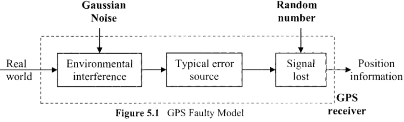
5.1 GPS Faulty Model 34 5.1.1 Typical Error Budget 34

5.1.2 Environmental Interferences 37

5.1.3 Signal Loss 37 5.1.4 Hardware Malfunction 38

5.1.5 Faulty Model Diagram 38

5.2 IMU Faulty Model 38 5.2.1 Errors Sources and Faulty Scenarios 38

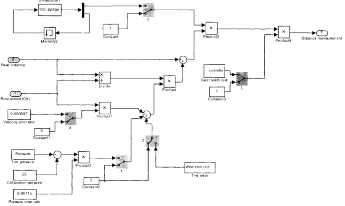
5.2.2 Faulty Model Diagram 39 5.3 Odometer Faulty Model 39

5.3.1 Tire Radius Change 40 5.3.2 Road Situation 40 5.3.3 Gears Tooth Loss 41 5.3.4 Faulty Model Implementation 41

5.4 Inclinometer Faulty Model 42 5.5 Magnetic Compass Faulty Model (Fluxgate Compass) 43

6 SENSORS FAULT DETECTION STRATEGIES

6.1 Fault Detection 45 6.2 Fault Monitoring System 46

6.3 Fault Detection and Diagnosis Theory 47

6.3.1 Hardware Redundancy 47 6.3.2 Analytical Redundancy 48 6.4 Proposed Fault Detection Method (model-based) 53

7 ADAPTIVE DATA FUSION STRATEGY

7.1 Adaptive Data Fusion Architecture 54 7.2 State Space Model of the Vehicle Dynamics 56

7.3 Adaptive Sensor Fusion System 60

7.4 Flow Chart 61 7.5 Threshold Determination 63

8 TEST RESULTS A N D PERFORMANCE ANALYSIS

8.1 Simulation Configuration 64 8.2 Sensors Faulty Models Performance 65

8.2.1 GPS Faulty Model Performance 66 8.2.2 IMU Faulty Model Performance 70 8.2.3 Odometer Faulty Model Performance 71 8.2.4 Inclinometer Faulty Model Performance 72 8.2.5 Magnetic Compass Faulty Model Performance 73 8.3 Adaptive Data Fusion Architecture Performance 74

8.3.1 Centralized Fusion-Centralized Fault Detection (CF-CFD)

Performance 74 8.3.2 Centralized Fusion-Decentralized Fault Detection (CF-DFD)

8.3.3 Decentralized Fusion-Decentralized Fault Detection (DF-DFD)

Performance 82 8.3.4 Discussion and Performances Comparison 85

9 CONCLUSIONS

9.1 Summary 87 9.2 Conclusions 87 9.3 Future Works 88

LIST OF TABLES

Table 1.1 Reason for Sensor Fusion 3 Table 3.1 Relationship of Vehicle Position and Sensor Outputs 10

Table 3.2 Definition of Sensor Characteristics / / Table 3.3 Comparison of low cost Gyroscope Technologies 15

Table 4.1 Performances Comparison between Centralized and Decentralized Fusion 25 Table 5.1 GPS Error Sources and their Approximate Deviation [Jon Kronander, 2004] 34

Table 8.1 Position Errors Statistic Performances 68 Table 8.2 Position Errors Statistic Performances (with signal loss) 70

Table 8.3 Attitude Errors Statistic Performances 70 Table 8.4 Distance Error Statistic Performances 71 Table 8.5 Inclination Error Statistic Performances 72

Table 8.6 Azimuth Error Statistic Performances 73 Table 8.7 Position Errors Statistic ofCF-CFD (no signal loss) 76

Table 8.8 Position Errors Statistic ofCF-CFD (with signal loss) 78 Table 8.9 Position Errors Statistic of CF-DFD (no signal loss) 80 Table 8.10 Position Errors Statistic of CF-DFD (with signal loss) 82 Table 8.11 Position Errors Statistic of CF-DFD (no signal loss) 83 Table 8.12 Position Errors Statistic of CF-DFD (with signal loss) 85 Table 8.13 Performance Comparison of Adaptive Fusion Architectures (no signal loss) 85

Table 8.14 Performance Comparison of Adaptive Fusion Architectures (with signal loss) 85

LIST OF FIGURES

Figure 2.1 Rectangular Coordinates 6 Figure 2.2 Geodetic and Rectangular Coordinates 7

Figure 2.3 SAE Coordinates 8 Figure 2.4 ENU Coordinates 8 Figure 3.1 Bubble Inclinometer [Harvey R., 1998] 13

Figure 3.2 Gimbaled IMU- 14 Figure 3.3 Spring and Pendulum Accelerometers [Savage 1978] 17

Figure 3.4 Toroidal Wound Fluxgate Compass Sensor [Ganssle J., 1989] 19

Figure 3.5 Satellite Constellation and Orbital Planes 20

Figure 3.6 GPS Positioning Principle 21 Figure 3.7 Real-time Differential GPS 22

Figure 4.1 Centralized Fusion 24 Figure 4.2 Decentralized Fusion 24 Figure 4.3 Kalman Filter 28 Figure 4.4 Nominal and Actual Trajectory for a Linearized Kalman Filter 29

Figure 4.5 Nominal and Actual Trajectory for an Extended Kalman Filter 31

Figure 4.6 A Complete Picture of the Operation ofEKF 32

Figure 5.1 GPS Faulty Model 38 Figure 5.2 IMU Faulty Model 39

Figure 5.3 Odometer Faulty Model 41 Figure 5.4 Inclinometer Faulty Model 42

Figure 5.5 Magnetic Compass Faulty Model 44 Figure 6.1 Fault Detection Methodology 46 Figure 6.2 FDI Techniques Taxonomy 47 Figure 6.3 Kalman Filter Based Fault Detection Architecture 53

Figure 7.1 Centralized Fusion - Centralized Fault Detection Architecture (CF-CFD) 54 Figure 7.2 Centralized Fusion - Decentralized Fault Detection Architecture (CF-DFD) 54 Figure 7.3 Decentralized Fusion - Decentralized Fault Detection Architecture (DF-DFD) 55 Figure 7.4 Decentralized Fusion - Centralized Fault Detection Architecture (DF-CFD) 55

Figure 7.5 Integrated Random Walk PVA Model 56 Figure 7.6 Integrated Gauss-Markov PVA Model 56 Figure 7.7 Integrated Gauss-Markov PV Model 57

Figure 7.9 Adaptive Sensor Fusion System 61 Figure 7.10 Adaptive Sensor Fusion Architecture Flow Chart 62

Figure 8.1 Trajectory 65 Figure 8.2 GPS Latitude 66 Figure 8.3 GFS Longitude 67 Figure 8.4 GPS Altitude 67 Figure 8.5 GPS Latitude (with signal loss) 68

Figure 8.6 GPS Longitude (with signal loss) 69 Figure 8.7 GPS Altitude (with signal loss) 69 Figure 8.8 Distance Measurements with Odometer 71

Figure 8.9 Inclination Measurements 72 Figure 8.10 Azimuth Measurements 73 Figure 8.11 Estimate of CF-CFD Architecture (no signal loss) 75

Figure 8.12 Estimated Trajectory of CF-CFD Architecture (no signal loss) 75

Figure 8.13 Estimate of CF-CFD Architecture (with signal loss) 77 Figure 8.14 Estimated Trajectory of CF-CFD Architecture (with signal loss) 77

Figure 8.15 Estimate of CF-DFD Architecture (no signal loss) 79 Figure 8.16 Estimated Trajectory of CF-DFD Architecture (no signal loss) 80

Figure 8.17 Estimate of CF-DFD Architecture (with signal loss) 81 Figure 8.18 Estimated Trajectory of CF-DFD Architecture (with signal loss) 81

Figure 8.19 Estimate of DF-DFD Architecture (no signal loss) 82 Figure 8.20 Estimated Trajectory of DF-DFD Architecture (no signal loss) 83

Figure 8.21 Estimate of DF-DFD Architecture (with signal loss) 84 Figure 8.22 Estimated Trajectory of DF-DFD Architecture (with signal loss) 84

ACRONYMS ABS ALI CACS CKF DARPA DGPS DKF DOP DOD DR ECEF EKF ENU FDI GNSS GPS GIS IMU INS ITS KF LKF LL LTP LTY MPH NEC NED NN PDOP PVA

Antilock Brake System

Autofahrer leit und Informations System

Comprehensive Automobile Traffic Control System Centralized Kalman Filter

Defense Advanced Research Projects Agency Differential GPS

Decentralized Kalman Filter Dilution of Precision

Department of Defence Dead Reckoning

Earth-Centered Earth-Fixed coordinate Extended Kalman Filter

East-North-Up coordinate Fault Detection and Isolation Global Navigation Satellite System Global Positioning System

Geographic Information System Inertial Measurement Unit Integrated Navigation System Intelligent Transportation Systems Kalman Filter

Linearized Kalman Filter Latitude/Longitude Tangent Plane Local Tangent Plane Miles Per Hour

Network of Centres of Excellence North-East-Down coordinate Neural Network

Position DOP

PV Position-Velocity SA Selective Availability

SAE Society of Automobile Engineer UWB Ultra-wideband

WGS84 World Geodetic System 1984 ZUPTs Zero-Velocity Updates

Chapter 1

INTRODUCTION

1.1 Research Context in Networks of Centres of Excellence AUT021

The present research project is financed by the NCE (Network of Centres of Excellence) A U T 0 2 1 . This network currently supports 36 research projects, over 230 top researchers working at more than 37 Canadian academic institutions, government research facilities and private sector research laboratories across Canada and around the world.

The Government of Canada established the Networks of Centres of Excellence program in 1989 to improve and enhance Canada's position in multitude of areas. Fostering powerful partnerships between university researchers, government and industry, the networks are designed to help develop Canada's economy and improve the quality of life for Canadians.

With an annual research budget of approximately $12 million, AUT021 and its private and public-sector partners fund innovative projects in a variety of areas. This research falls within the following six key areas that enable key topics to be explored:

• Health Safety and Injury Prevention • Societal Issues

• Materials & Manufacturing • Powertrains, Fuels & Emissions • Design Processes

• Intelligent Systems and Sensors

The present research falls in the topic Intelligent System & Sensors, and is carried out with the FII project (Intelligent Information & Navigation System), which is leaded by Dr. Elizabeth Cannon at the University of Calgary.

1.2 Background

Mobility is an essential requirement for any type of meaningful involvement in our modern society. Without mobility, an individual's chances for participation in this country's socioeconomic system are severely limited. Since most jobs are not in close proximity to home, the chances of a person attaining gainful employment, without

possible for people to shop, to socialize, to worship, or to participate in many other life-enriching activities.

With more and more people having vehicles of their own, surface vehicle ownership and the use of vehicles are growing at rates much higher than the rate at which roads and other infrastructures are being expanded. As the number of vehicles increases, many challenges are also encountered: chronic traffic congestion at the peak hours, road accidents, and automobile exhaust pollution. In order to improve vehicle transportation infrastructure, intelligent transportation systems (ITS) are proposed. This exciting new field is an integration of computers, information, and communication technologies.

The objective of ITS is to apply advanced technologies to make transportation operate more safely and efficiently, with less congestion, pollution, and environmental impact. The theory and practice of ITS are currently among the most intensely studied and promising areas in transportation, computer, information, communication, and systems science and engineering, and one that will certainly play a primary role in our future lives.

During the past decade, vehicle location and navigation systems and other ITS-related systems have been rapidly gaining momentum worldwide. In Japan, the ITS movement began in 1973 with the Comprehensive Automobile Traffic Control System (CACS); in Europe, the ITS started in the late 1970s with Autofahrer leit und Informations System (ALI) project; in the United States, an autonomous navigation system called Navigator was proposed and developed commercially in the mid-1980s [Yilin Zhao, 1997].

Modern vehicle location and navigation systems basically consist of wireless communications, route planning, route guidance, human-machine interface, digital map database, map matching and vehicle positioning [Yilin Zhao, 1997]. The positioning module is a vital component of any vehicle location and navigation systems, and it usually consists of multiple sensors. These sensors have different characteristics making it possible to provide the information, either complementary, or redundantly with an aim of improving the performance of the positioning module. With this intention, the unmined data obtained from various sensors must be amalgamated. Data fusion, which has been defined by the Defense Advanced Research Projects Agency (DARPA), as an information processing method that deals with the association, correlation, and combination of data and information from single and multisources to achieve refined

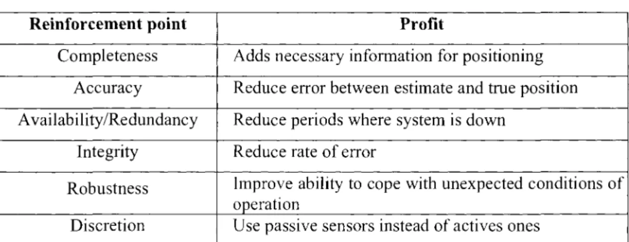
position and identity estimation, complete and timely assessments of situations and threats, and their significance in the context of mission operation. The benefits of data fusion are listed in Table 1 [Francois, 2003].

Table 1.1 Reason for Sensor Fusion Reinforcement point Completeness Accuracy Availability/Redundancy Integrity Robustness Discretion Profit

Adds necessary information for positioning Reduce error between estimate and true position Reduce periods where system is down

Reduce rate of error

Improve ability to cope with unexpected conditions of operation

Use passive sensors instead of actives ones

In positioning navigation system, high precision and reliability with low cost are always pursued. Actually, for road navigation, the benefit of the information obtained by the fusion process makes it possible to have multiple less powerful, low cost sensors to achieve as good a performance as those much more expensive ones. Moreover, sensor fusion provides a system with additional benefits, which may include robust operational performance, an increased degree of confidence, improved detection performance, improved reliability of system operation, full utilization of resources, and reduced ambiguity.

1.3 Problem Specification

Generally speaking, a conventional data fusion architecture can be used to fuse data from different sensors so as to obtain the vehicle position. But as a matter of fact, in positioning navigation system, at any time, any of the sensors can be corrupted or break down temporarily or permanently. Let say Global Positioning System (GPS), which is a line-of-sight sensor, tends to be sensitive to situations with limited sky visibility. Such situations include: urban environments with tall buildings; inside parking structures; underneath trees; in tunnels and under bridges. In such cases, the sensor faults or performance degradation will tend to degrade even paralyze the navigation solution. As a result, it may present hazards to drivers and passengers or lead to unacceptable economic

of the fault or failure must be detected and isolated from the system, and finally the system must be able to reconfigure itself so as to overcome the deficiency caused by the sensor fault or failure. In brief, a navigation system must be robust and adaptive.

The general objective of this thesis is to find robust solutions to the positioning navigation problem using common sensors available in automotive environments, such as:

• GPS

• Inertial Measurement Unit (IMU) • odometer

• inclinometer • magnetic compass

Of special interest is the performance in scenarios where conventional positioning methods do not apply, or have a general degradation of performance, e.g., when one or multiple of the moving parts of the IMU wear out or jam. Another important issue is situations where the GPS input is temporarily blocked, or corrupted in some other way. Examples of such situations are:

• urban environments with tall buildings ("Urban canyons") • inside parking structures

• in tunnels

• under heavy foliage • under bridges

1.4 Objectives

The main purpose of this research project is to develop and implement adaptive positioning modules that fuse information from the GPS receiver, IMU, odometer, inclinometer and magnetic compass to provide robust positioning navigation solutions. To achieve the main objective, the following issues have to be considered:

• Sensor faults and performance degradations models have to be proposed and implemented from the relevant driving scenarios.

• Fault detection and isolation model have to be investigated.

• Robust positioning data fusion solution has to be developed and implemented. • Performance analysis has to be carried out to the proposed solution.

1.5 Limitations

The proposed algorithms are approaches based on Kalman filter, it is necessary to have the apriori knowledge about noise distribution of the position sensors. In a real driving situation, it is difficult, or sometimes impossible, to know previously the distribution of the noise.

One more limitation is that the thresholds for the sensor fault detection are empirical.

1.6 Thesis Outline

Chapter 2 introduces different coordinate systems used in this thesis, and also their conversion. Chapter 3 explains various positioning sensors employed to sense data for the fusion architecture in this thesis. Chapter 4 addresses the theory used for the sensor fusion, starting with fusion architectures and concluding with Extended Kalman Filter. Chapter 5 studies the sensor fault or failure scenarios and performs their implementation. Chapter 6 presents the sensor fault detection strategies, including the basic knowledge introduction and further exploration. Chapter 7 investigates the adaptive data fusion solution, with combining sensors faults detection and data fusion into a single architecture. Chapter 8 carries out performance analysis for the sensors faulty models and the proposed adaptive solutions. The conclusions are summarized in Chapter 9, along with suggestions for future work.

Chapter 2

C O O R D I N A T E SYSTEMS

When designing a multi-sensor navigation system, it is necessary to relate the information from the different sensors to a single navigation coordinate system. In this thesis, the Earth-Centered Earth-Fixed (ECEF) frame is used together with the local tangent plane frame and the body-fixed vehicle frame.

2.1 ECEF Coordinates

The Earth-Centered Earth-Fixed (ECEF) coordinate system is a three-dimensional Cartesian coordinate system. The origin of this system is at the centre of mass of the Earth - well defined by observing the orbits of satellites together with gravity measurements. Its x-axis and y-axis coincide with the plane of zero latitude, and the z-axis coincides with the Earth's rotational z-axis. The x-z-axis also passes through the point of zero longitude (the prime meridian). Two coordinate systems are used in the ECEF frame: rectangular and geodetic.

2.1.1 Rectangular coordinates

The x-axis of this system extends through the prime meridian (0° longitude) and the equator (0° latitude). The z-axis extends through the north pole, parallel to the Earth's spin axis. The y-axis completes the right-handed coordinate system.

Prime Meridian

Equator

2.1.2 Geodetic Coordinates

A geodetic coordinate system (sometimes called geographic coordinate system) is an angular coordinate system consisting of an ellipsoid, the equatorial plane of the ellipsoid, and a meridional plane through the polar axis of the ellipsoid (Figure 2.2). The coordinates of a point in this system are given by the perpendicular distance of the point from the ellipsoid (the ellipsoidal height h), by the angle between that perpendicular (the normal) and the equatorial plane (the geodetic latitude <P), and by the dihedral angle between the meridional plane and a plane perpendicular to the equatorial plane and containing the normal (the geodetic longitude X). This system designates a point with respect to the reference ellipsoid and with respect to the planes of the geodetic equator and a selected geodetic meridian. The geodetic equator is an ellipse on the reference ellipsoid midway between its poles of rotation. This equator is the line on which geodetic latitude is 0 degrees, and from which geodetic latitudes are reckoned, North and South, to 90 degrees, at either pole. If the minor axis of the reference ellipsoid is parallel to the rotational axis of the Earth, the geodetic equator will coincide with the Earth's equator.

Most position information from navigation tools is expressed in geodetic coordinates. There are several ellipsoid models of Earth. Perhaps the most widely used, mainly because GPS is based on in it, is the World Geodetic System 1984 (WGS84). In addition to a major and minor axis, WGS84 specifies a gravitational constant and an angular velocity (rotation of the Earth).

2.2 RPY Coordinates

The RPY coordinates are vehicle fixed, with the roll axis in the nominal direction of motion of the vehicle, the pitch axis out the right-hand side, and the yaw axis such that turning to the right is positive, as illustrated in Figure 2.3. This frame is suitable for the description of basic vehicle dynamics and the derivation of related equations of motion. This is also called "SAE coordinate," because it is the standard body-fixed coordinate used by the Society of Automotive Engineer.

Y Roll Axis Yaw Axis

Figure 2.3 SAE Coordinates

2.3 ENU/END Coordinates

East-North-Up (ENU) and North-East-Down (NED) are two common right-handed Local Tangent Plane (LTP) coordinate systems. In ENU coordinates, altitude increases in the upward direction; while in NED coordinates, the direction of a right turn is in the positive direction with respect to a downward axis [Mohinder S. Grewal et coll., 2001].

2.4 Conversion

The useful transformation matrix that relates the RPY frame and the local geographic frame can be obtained with the following integration [Mohinder et coll., 2001]:

~sin(y)cos(P) cos(^)cos(7)+sin(R)sm(Y)sm(p) - sin(fl)cos(r)+ cos(/?)sin(y)sin(P)~

CMI= cos(7)cos(P) -cos(i?)sin(r)+sin(7?)cos(7)sin(/') sin(/?)sin(r)+cos(/?)cos(r)sin(p)

sin(p) -sin(i?)cos(/>) -cos(tf)cos(>) (2.4.1)

Chapter 3

P O S I T I O N I N G SENSORS

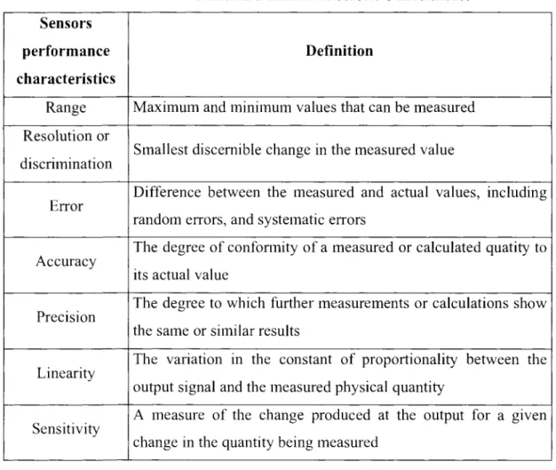
To be useful, systems must interact with their environment. To achieve this objective, in positioning navigation system, various sensors are used. A sensor is a device that responds to or detects a physical quantity and transmits the resulting signal to a controller. Position sensors can be designed to detect various variables (coordinates, distance, direction, or angular velocity) of the position of vehicular mechanical systems (detail relationship is shown in Table 3.1). They are either directly coupled to a shaft or linkage, or indirectly coupled to these or other vehicle parts in the case of a non-contact or proximity sensor. Actually, a sensor has numerous interesting performances. Characteristics with definitions of the sensor performance are listed in Table 3.2.

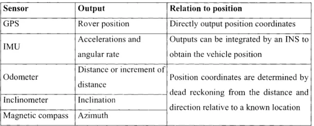
Table 3.1 Relationship of Vehicle Position and Sensor Outputs

Sensor GPS IMU Odometer Inclinometer Magnetic compass Output Rover position Accelerations and angular rate Distance or increment of distance Inclination Azimuth Relation to position

Directly output position coordinates Outputs can be integrated by an INS to obtain the vehicle position

Position coordinates are determined by dead reckoning from the distance and direction relative to a known location

Nowadays, all vehicles have an odometer, mechanical or electronic, to record the total distance traveling. Obviously, the odometer is a necessary and common sensor used in auto industry. However, only middle and high level automobiles are equipped with magnetic compass and inclinometer. As to GPS and IMU, although they are not so often being used in nowaday automobiles, they are the direction of develop and the objective to pursue.

Table 3.2 Definition of Sensors Characteristics Sensors performance characteristics Range Resolution or discrimination Error Accuracy Precision Linearity Sensitivity Definition

Maximum and minimum values that can be measured

Smallest discernible change in the measured value

Difference between the measured and actual values, including random errors, and systematic errors

The degree of conformity of a measured or calculated quatity to its actual value

The degree to which further measurements or calculations show the same or similar results

The variation in the constant of proportionality between the output signal and the measured physical quantity

A measure of the change produced at the output for a given change in the quantity being measured

3.1 Relative Position Sensors

A relative sensor is a device that can measure the change in distance, position, or heading based on a predetermined or previous measurement. Without knowing an initial position or heading, this sensor cannot be used to determine absolute position or heading with respect to the Earth. As an example, odometer, inclinometer, accelerometer, and gyroscope are all relative sensors.

3.1.1 Odometer

An o d o m e t e r is used to measure the distance traveled by a vehicle, or possibly by the individual wheels. Most vehicles have a transmission-based odometer to track the total distance or trip distance traveled by the car. This type of odometer counts the revolutions of the powertrain after the clutch or torque converter. The process of counting the revolutions often uses the coupling of mechanical and electrical forces or optics to detect

wheel rotation counts and multiplying by a proper scale factor enables the distance traveled by the vehicle to be determined. There can be any number of digital pulses (discrete) or sinusoids (continuous) accumulated per rotation of the shaft; some simple systems use one per rotation, while others accumulate hundreds for demanding applications such as Antilock Brake System (ABS) or traction control. Both wheel and transmission odometers can be used to aid in navigation application by providing speed, distance, and possibly heading information.

In order to improve the accuracy, differential odometers are used. In general, differential odometry is a technique to provide both traveled distance and heading change information by integrating the outputs from two odometers, one each for a pair of front or rear wheels. When a vehicle turns, the differential allows the inside tire to travel a shorter distance than the outside without greatly increasing slippage. Differential odometry uses the two wheel-based speed or distance measurements to estimate the change in heading. The individual wheel speeds would therefore vary from the GPS speed of the vehicle while it is turning.

As discussed previously, distance traveled over ground by the vehicle is mostly computed through averaging the two accumulated distances. The following equation is presented in [Yilin Zhao, 1997]:

d(t) = d(t-l)+KiC'-+K*CR (3.1.1.1)

where CL and CR are the number of counts for the left wheel and right wheel,

respectively. KL and KR are calibration constants which are proportional to the radius of

the tires. Unfortunately, the fact that tire radius is not strictly constant but varies slightly as the vehicle travels, introduces several potential error sources into the distance computation, and will tend to cause the odometer in a faulty state. This will be discussed further in Chapter 5.

3.1.2 Inclinometer

An inclinometer is a sensor used to measure the angle between the gravity vector and the platform to which it is mounted. This can be in a single direction, i.e. for sensing vehicle roll only, or two directions to estimate pitch, as well. Inclinometers suffer an error due to vehicle accelerations since it is not possible to separate them from the gravity vector. It

would be possible to make corrections to the inclinometer output using a gyroscope and a differential odometer to isolate the vehicle accelerations, but GPS code positioning cannot provide an accurate estimate of acceleration to compute this correction [Harvey R., 1998].

Inclinometers designed specifically for low cost environments such as automotive applications now cost around $10. A typical 2-axis bubble type inclinometer would be the Applied Geomechanics Model 900 Biaxial Clinometer, available at $90 in large quantities. The operation of this type of inclinometer will be described below.

The liquid-bubble inclinometer uses a vial, partially filled with a conductive liquid, to determine the tilt of the vehicle in one or more axes. Electrodes around the vial estimate the liquid height or height difference between sensors. These measurements are converted to pitch or roll measurements. A diagram of a typical sensor is found in Figure 3.1.

Liquid Surface Sensing ' Electrode 9 ' ^ B,t g + a.

Figure 3.1 Bubble Inclinometer [Harvey R., 1998]

One drawback of bubble inclinometers is their suffering from the acceleration related errors, which is due to the fact that vehicle acceleration will make the liquid rise up one side of the vial. Also, there will be some sort of damped oscillation in the fluid even after the acceleration has finished. The error due to vehicle acceleration can be found in [Jim Stephen, 2000]

where g is the magnitude of gravity and av is the acceleration of the vehicle.

3.1.3 Inertial Measurement Unit (IMU)

Inertial sensors make measurements of the internal state of the vehicle. A major advantage of inertial sensors is that they are non-radiating and non-jammable and may be packaged and sealed from the environment. This makes them potentially robust in harsh environmental conditions.

Historically, Inertial Navigation Systems (INS) has been used in aerospace vehicles, military applications such as ships, submarines, missiles, and to a much lesser extent, in land vehicle applications. Only a few years ago, the application of inertial sensing was limited to high performance high cost aerospace and military applications. However, motivated by requirements for the automotive industry, a whole variety of low cost inertial systems have now become available in diverse applications involving heading and attitude determination.

Definitely, an IMU contains a cluster of sensors: gyroscopes and accelerometers [Mohinder S. Grewal et coll., 2001]. These sensors are rigidly mounted to a common platform to maintain the same relative orientation. Specifically, inertial sensors measure rotation rate and acceleration, both of which are vector-valued variables:

Gyroscopes are sensors for measuring rotation: rate gyroscopes measure rotation rate,

and displacement gyroscopes measure rotation

^ccetfii-jrr«riarc .- «* t

Accelerometers are sensors for measuring ''••''..-* [ ^ " .^^

acceleration. However, accelerometers cannot f ^^fv- 'R,-,!r,w

measure gravitational acceleration. That is, an / 1 ^-J*""1

accelerometer in free fall has no detectable "" "*'" Mcunreji™-™ input. Figure 3.2 Gimbaled IMU

Gyroscopes

As described previously, a gyroscope is an instrument used to measure the rate of rotation or integrated heading change of a platform [Savage, P., 1978]. A single gyroscope measures rotation on a single plane, but a triad of gyroscopes is often mounted orthogonally in a single enclosure to monitor the three possible rotations in 3-D space. Quite a few different types of gyroscopes are available, ranging greatly in price and stability. Gyroscopes are classified into gimbaled or strapdown varieties, with gimbaled gyroscopes maintaining a fixed orientation in an inertial frame. Table 3.3 summarizes several different low cost gyroscope technologies for cost and accuracy.

Table 3.3 Comparison of low cost Gyroscope Technologies [Jim Stephen, 2000] Gyro Type Rotating Fiber Optic Vibrating Piezoelecric Principle of Operation Conservation of Angular Momentum Sagnac Effect Coriolis Effect Cost ($) 10-100 50-1000 10-200 Stability (7h) 1-100+ 5-100 50-100+

Comparing with the cost and stability, rotating model is more suited for automobile application. Strapdown gyros, the most common rotating model, measure rotation on a fixed plane with respect to the vehicle, which is not generally on the plane orthogonal to the gravity vector. Therefore, they do not sense the entire rotation in heading, but also sense rotations in pitch and roll. The formula that describes the relationship between the measured rotation rate and the desired rate of heading change is given in equation (3.1.3.1) [St. Lawrence, 1993].

coG = (Qy cos^ + co^ c o s / ? s i n £ + <z>e s i n / ? s i n ^ (3.1.3.1)

Rearranged for the heading rate, the result is

coG cov COS /?sin<^ + coe sin /? sin ^

c o s ^ c o s ^ where

coG is the measured rotation rate

(Ovv is the desired azimuth rotation rate

coe is the pitch rotation rate

O) is the roll rotation rate

p is the roll angle

r is the pitch angle

P is the horizontal component of the gyro and Latitude/Longitude (LL) plane

misalignment

£ is the misalignment between the gyro and LL vertical vectors

Accelerometers

An accelerometer measures platform acceleration, which can be integrated to give velocity, and double integrated to give distance traveled. Other uses for accelerometer data include the detection of impacts for air bag deployment, and inclination measurement through sensing of the Earth's gravitation. Vibration measurements are now being investigated to detect potential engine problems before further damage or failure results. Sensor drift makes regular ZUPTs (Zero-Velocity Updates) necessary for periods without an accurate external reference, since the double integral can accumulate substantial errors. The drift is mostly temperature related, so investigation into the various compensation schemes has been done. The use of constant-temperature ovens can ensure good stability after warm-up, but an oven uses a great deal of power and much larger space. Another technique is to generate a temperature profile and count on temperature repeatability; this can be done a priori or built up over time in a real-time application.

Accelerometers are generally based on observing the displacement of a suspended mass caused by inertia. Two common implementations, a damped spring and pendulum, are shown in Figure 3.3. Methods such as differential capacitance, inductance, or optical methods can be used to measure the displacement. Sometimes a magnetic field or servo is employed to keep the mass in fixed position. Purely optical methods of measuring acceleration, similar to those used in optical gyros, have been developed recently, as well.

No Acceleration

No Acceleration

Spring Pendulum

Figure 3.3 Spring and Pendulum Accelerometers [Savage 1978]

A damped spring will allow the suspended mass to displace under an acceleration. The movement of the mass would be sensed through capacitance, an optical method, or otherwise, while damping is usually accomplished by the use of a viscous fluid medium. The accelerometer described in this example can be modeled with a second order equation [Jim Stephen, 2000]:

F = m(^)+c(^)+Kx (3.1.3.3)

where

F is the applied force

m is the mass of the suspended mass

c is the damping coefficient (a function of the medium) K is the spring stiffness

x is the displacement of the spring relative to resting position

On the other hand, a resting pendulum will also displace under an acceleration, moving further up its arc with greater acceleration. The motion is again usually damped by the medium. The amount of displacement depends on the weight distribution in the pendulum, but assuming the mass is all at the bottom of the arm, the arm would point in

the same direction as the sum of the gravity and acceleration vectors. Angular or linear displacement of the mass could be measured using one of the methods mentioned above.

3.2 Absolute Position Sensors

Absolute position sensors are very important in solving location and navigation problems. As mentioned previously, a relative sensor alone cannot provide an absolute direction or position with respect to a reference coordinate system. In contrast, the output of the absolute sensor is always relative to a fixed reference, regardless of the initial conditions. Therefore, an absolute sensor can provide information on the position of the vehicle with respect to the Earth. The most commonly used technologies for providing absolute position information are the magnetic compass and GPS [Yilin Zhao, 1997].

3.2.1 Magnetic compasses

A magnetic compass measures the direction of the Earth magnetic field. This physical principle has been used since the 1200s to navigate ships across the ocean. An original compass consisted of an iron needle floating in water, but it has been developed a lot to date. When used in a positioning system, a compass measures the orientation of an object to which the compass is attached. The orientation is measured with respect to magnetic North. The compass information needs to be corrected because of the discrepancy between the true North and the direction of the Earth's magnetic field. Another correction is also required due to vertical magnetic equator and maximum at the poles.

The magnetic compass is the only low cost absolute heading reference presently available for the automotive market. Other absolute references, such as North-seeking gyros, are far too expensive. The serious drawback for the use of a magnetic compass on a vehicle is the hostile magnetic environment of an automobile. Several manufacturers, including KVH Industries Inc., have built gyro stabilized compasses which blend the short term relative accuracy of gyro with the absolute sensing of a compass for an improved heading sensor.

A magnetic compass senses the magnetic field of the Earth on two or three orthogonal sensors, sometimes in conjunction with a biaxial inclinometer. Since this field should

point directly North, some method can be used to estimate the heading relative to the magnetic North pole. There is a varying declination between the magnetic and geodetic North poles, but models can easily generated this difference to better than one degree. The magnetic sensors are usually flux-gate sensors; one of which is pictured in Figure 3.4.

Figure 3.4 Toroidal Wound Fluxgate Compass Sensor [Ganssle J., 1989]

The operation of a fluxgate is based on Faraday's law, which states that a current (or voltage) is created in a loop in the presence of a changing magnetic field (Ganssle J., 1989). A fluxgate is composed of a saturating magnetic core, with a drive winding and a pair of sense windings on it (only one is shown in the figure). The drive winding is wrapped around the core, which is normally a toroid. These sense windings are often wound flat on the outside of the core and are arranged at precisely 90° to each other. When not energized, a fluxgate's permeability 'draws in' the Earth's magnetic field [Ripka P., 1992)]. When energized, the core saturates and ceases to be magnetic. As this switching occurs (hence the name fluxgate), the Earth magnetic field is drawn into or released from the core, resulting in a small induced voltage that is proportional to the

3.2.2 Global Positioning System (GPS)

The GPS is a satellite navigation system conceived, designed and operated by the US Department of Defence (DoD). A GPS consists of three main parts: the space segment -satellites, the control segment - management and control, and the user segment - receiver [YilinZhao, 1997].

• Space segment: 24 operational satellites are in six circular orbits 20,200 km above the Earth with a 12-hour period. The satellites are spaced in orbit so that 98% to 100% of the time a minimum of 6 satellites will be in view of users anywhere in the world. The satellites continuously broadcast position and GPS time data.

Figure 3.5 Satellite Constellation and Orbital Planes

Control segment: The control sub-system is made up of several stations on Earth, where GPS satellite trajectories are monitored and time is recalculated with great precision. Using this data, the computerized system on each satellite recalculates and corrects its position and then corrects the information sent to Earth. The primary control station of the GPS constellation is situated in Colorado Springs in the USA, which is used to track all GPS satellites and compute precise satellite orbits so as to produce information that is then formatted into updated navigation messages.

User segment: The equipment consists of a radio receptor with a processing unit that decodes information sent by each satellite in real time and computes the precise position, velocity and time. This is performed using the time delay for the signal to reach the receiver, which is the direct measure of the apparent range to

the satellite. A total of at least four satellites reading are needed to solve for the three dimensions of space and the time of the receiver.

The GPS intends to be used for precise positioning through the determination of pseudoranges from the satellites to the receiver. The key idea is that by measuring the time of flight of a radio signal from 4 or more satellites to the receiver, the position of the receiver may be accurately determined. In addition the time offset of the receiver may be calculated from information within the orbit data. As a simple example, the 3-D position of the receiver can be evaluated using standard triangulation techniques with range observations from at least four satellites. The position of the satellites is predicted with the ephemeris information. With time stamp range and satellite position information the following set of non-linear equations can be stated to obtain the 3-D position of x, y and z, and the GPS receiver clock drift At [Nebot E., 1999].

Satellite 2 Q Q Satellite 3 (x3, y3, z3) Satellite 4

O

Figure 3.6 GPS Positioning Principle

' ( - /(*-- , )2

--rj

-*,Y

(y-+ 0"

-yj

~z

f

~zj

u = V ( * - 0

+ (y-yJ + (

-zJ + cAt

where c is the speed of light.

Differential GPS uses position corrections to attain greater accuracy. It does this by

the use of a reference station, which is configured as in Figure 3.7. The reference station (or base station) may be a ground based facility or a geosynchronous satellite, in either case it is a station whose position is a known point. When a station knows what its precise location is, it can compare that position with the signals from the GPS satellites and thus find the Selective Availability (SA) error. These corrections can then be immediately transmitted to mobile GPS receivers (real-time DGPS), or the receiver positions can be corrected at a later time (post processing).

and transmitter

Figure 3.7 Real-time Differential GPS

Obviously, the use of DGPS can greatly increase positional accuracy. But as usual, the better it is the more expensive it is. Some surveying systems can even give subcentimeter readings. As a matter of fact, there are a lot of different differential providers that supply real-time and post processing corrections, many of them are private companies. The availability of these services varies greatly depending on what part of the country one is in, but the Natural Resources Canada along with its public, private and board partner provide an accessible range from coast-to-coast, beyond the U.S. border, and into the Arctic.

Chapter 4

SENSOR FUSION

While GPS provides bounded errors for position and velocity, GPS users experience signal blockage; interference or jamming. As GPS signal is coining from about 22,000 km from the sky, it is relatively weak and affected by the atmosphere, line of sight and etc. In spite of many successful research activities to handle identified error sources such as ionosphere modeling, multipath mitigation and DGPS, the visibility to adequate number of GPS satellites from the recipient is still critical in using GPS alone navigation devices. Under the tree, inside the building, in the tunnel, and between the tall buildings, GPS positioning becomes difficult due to the signal blockage and degradation. Limitations of GPS enforce one to integrate multiple navigation sensors to provide the on-vehicle system with complementary, sometimes redundant information for its location and navigation task. To fuse the complementary information from different sources into one representation format, sensor fusion technologies had been developed. General speaking, sensor fusion is a method for conveniently integrating data provided by various sensors, in order to obtain the best estimate for a dynamic system states. In vehicle navigation system, sensor fusion algorithms are particularly useful in low-cost applications, where acceptable performance and reliability is desired, given a limited set of inexpensive sensors.

This section presents the fusion architectures, state space model and the most popular data fusion methods for vehicle positioning system, namely Kalman filter (KF) and its derivatives.

4.1 Fusion Architecture

It is well known that there exist two dissimilar architectures for data fusion: centralized and decentralized. The Centralized Kalman Filter (CKF) is the most common filter design implemented in integrated navigation systems such as those of United States Air Force aircraft today. The CKF receives all available measurements and combines all the information contained in those measurements to obtain an optimal navigation solution. For example, when applied to the well-modeled linear systems, the CKF is

When considering tradeoffs of data flow, algorithmic requirements, and processing speed versus optimality, fault tolerance, estimation in a multi-sensor environment is often best treated as a distributed estimation problem. The Decentralized Kalman Filter (DKF) architectures employ a bank of local Kalman filters dedicated to the sensors that provide measurement information to the system. A master filter combines the estimates from the bank of filters to obtain a typically suboptimal navigation solution. This poses less of a computational burden per filter than a centralized filter implementation. Although these estimates are typically slightly suboptimal, the distributed filter offers improvements over the centralized fault detection and isolation schemes.

In brief, employing centralized architecture, all sensor measurements are fused directly by one global fusion method; while employing decentralized architecture, after being filtered by individual local filter, local estimation positions are produced. Then all the outcomes are fused by a global fusion method and the desirable estimation position is finally procured [Mathieu St-Pierre et coll., 2004; Francois Meers, 2003].

GPS — I MU Odometer Inclinometer Magnetic compass Fusion Method Estimation Position

Figure 4.1 Centralized Fusion

GPS MU • Odometer Inclinometer Magnetic compass Filter 1 Filter 2 Filter 3 Filter 4 Filter 5 ^ n X?2 ^ «

*„

Method Estimation _Position

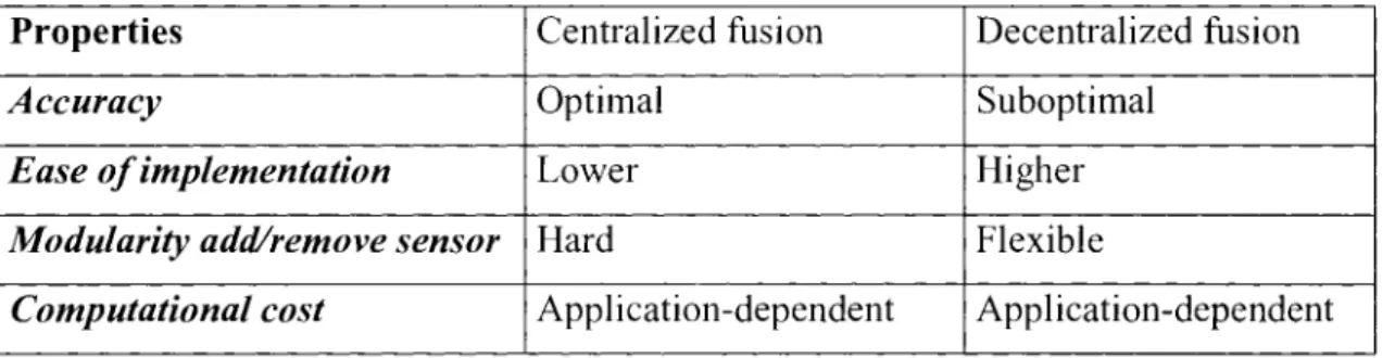
The following Table 4.1 shows the performance comparing between both fusion architectures [Francois Meers, 2003].

Table 4.1 Performances Comparison between Centralized and Decentralized Fusion Properties

Accuracy

Ease of implementation Modularity add/remove sensor

Computational cost Centralized fusion Optimal Lower Hard Application-dependent Decentralized fusion Suboptimal Higher Flexible Application-dependent

4.2 State Space Model

State space model is essentially a notational convenience for dynamic estimation and control problems, developed to make tractable what would otherwise be a notationally-intractable analysis. Begin with considering a dynamic process described by an n-th order difference equation (similarly a differential equation) of the form [Greg Welch et coll., 2001]

yk+\ =ao.kyk+- + a„-i,kyk-n+i+lik>k^() ( 4 2 1 ) where {a,. } is a zero-mean white random noise process with autocorrelation

E(uk^i) = Ru=QkSk, ( 4 2 2 )

and initial values {y {), y _\,..., y_„ + ] } are zero-mean random variables with a known

n x n covariance matrix

P^Eiy^y^l l,me{0,n-l} (4.2.3)

Also assume that

E(uk,yk) = 0 for-n + \<!<0 andk>0

which ensures that

E{uk,yk)=0 k>l>0 (4.2.5)

In other words, the noise is statistically independent from the process to be estimated. Under some other basic conditions, this difference equation can be re-written as a linear system:

xk+\ -yk yk-\ yk-n + 2 1 0 . . . 0 0 0 1 . . . 0 0 0 0 . . . 1 0

I" y

+

V

which leads to the state-space model

* A + I = Axk + Guk (4.2.7)

(4.2.8) yk =Htxk

where uk = [l 0... o].

Equation (4.2.7) represents the way a new state xk+l is modeled as a linear

combination of both the previous state xk and some process noise uk . Equation (4.2.8)

describes the way the process measurements or observations yk are derived from the

internal state xk. These two equations are often referred to respectively as the process

model and the measurement model, and they serve as the basis for virtually all state space

linear estimation methods, such as the Kalman filter described below.

4.3 Kalman Filter

Kalman filtering has been used extensively in autonomous or assisted navigation data processing for several decades. It is a set of mathematical equations that provides an efficient computational means to estimate the state of a process, in a way that minimizes the mean square error. This filter is very powerful in several aspects: it supports estimations of past, present, and even future states, and it can do so even when the precise nature of the modeled system is unknown.

As one of the most popular data fusion methods, the recursive implementation of Kalman filter is well suited to the fusion of data from different sources at different times in a statistically optimal manner. Many other filter designs can be shown to be equivalent to the Kalman filter, given several constraints. The recursive sequence involves prediction and update steps. The prediction step used a dynamics model that describes the relationship between variables over time. A statistical model of this dynamic process is

also necessary. A prediction is usually done to estimate the variables at the time of each measurement, as well as in between measurements when an estimate is required. The measurement update combines the historical data passed through the dynamics model with the new information in an optimal fashion.

The Kalman filter addresses the general problem of trying to estimate the state

x e dl" of a discrete-time controlled process that is governed by the linear stochastic

difference equation (with no loss of generality we will consider that the system has no external input) [Greg Welch et coll., 2001]

**+i =<Pkxk+™k (4-3.1)

with a measurement z e SI'" that is

Zu=Hkxk+vk (4.3.2)

The random variables wk and vk represent the generating process and measurement

noise, respectively. They are assumed to be independent, white, and with normal probability distributions

p(w)~N(0,Q) (4.3.3) p{y) ~ N(0, R) (4.3.4)

Supplied with initial conditions P0 andx0 , the prediction equations can be given by

* *+I = A * A (4-3-5)

P^=A-PJl+Qk (43.6)

and the update equations by

Kk=PkHl(HkP-H[+RkY (4.3.7)

*k =x~k+K(zk-Hkx-) (4.3.8)

Pk=(l-KkHk)Pk (4.3.9)

where

x is the vector of estimated states P is the covariance of estimated states Q is the dynamics noise matrix

z is the vector of observations

H is the measurement matrix

^ is the state transition matrix

Graphically, the operations of the Kalman filter can be outlined as in Figure 4.3 [Mathieu St-Pierreet coll., 2004].

Although an error state Kalman filter is desirable in some applications, a state space model will be preferred here as it most clearly illustrates the operation of the filter. Rigorous development of a Kalman filter requires a great deal of work in understanding the physics and electronics involved in each sensor to understand what the error sources will be. A comprehensive model of all of the necessary variables to match as closely as possible the real world phenomenon is needed. Given the specifications of the project, a sensitivity analysis would then be done to decide which variables may be ignored or lumped together. This often involves Monte Carlo simulations with several likely candidate filters and repeated tuning of the statistics. The filter must be able to operate with the allowed throughput and processing restrictions. Finally, blunder detection, adaptive filter gains, and practical limits to covariance must be set to achieve optimum performance.

4.4 Linearized Kalman Filter (LKF)

As described in the previous section, the Kalman filter deals with the general problem governed by a linear stochastic difference equation. But what happens if the process to be estimated and/or the measurement relationship to the process are nonlinear?

Actually, some of the most successful applications of Kalman filtering have been in situations with nonlinear dynamics and/or nonlinear measurement relationships. There are two basic ways of linearizing the problem. One is to linearize about some nominal trajectory in state space that does not depend on the measurement data. The resulting filter is usually referred to as simply a linearized Kalman filter. The other method is to linearize about a trajectory that is continually updated with the state estimates resulting from the measurements. When this is done, the filter is called an extended Kalman filter, which will be presented in next section.

Supposing the process to be estimated and the associated measurement relationship are given by [Robert Grover Brown et coll., 1997]

x = f(x,t)+w(t) (4.4.1) z = h(x,t)+v(t) (4.4.2)

where / a n d h are known, both or either nonlinear functions, and w and v are white-noise processes with zero crosscorrelation as before.

As shown in Figure 4.4 [Robert Grover Brown et coll., 1997], assume that the actual trajectory can be determined by the nominal or reference trajectory and the difference, then leads to

A c t u a l Trajectory x (t)

Ax

. ' Nominal Trajectory x* (t)

(Actual) - (Nominal) = Ax (t)

x(t) = x*(t) + Ax

equations (4.4.1) and (4.4.2) then become

x* + Ax = f[x* + Ax, t)+ w(t) z - h(x* + Ax,t)+v(t)

the first order Taylor series expansion gives

df

It is customary to choose the nominal trajectory x* (t) to satisfy the deterministic differential equation

x=f(x\t) (4.4.9)

Substituting (4.4.9) into (4.4.6) and (4.4.7) then leads to the linearized model [Robert Grover Brown et coll., 1997]

Ax

dx • Ax + w{t) (linearized dynamics) (4.4.10)

[z-h(x*,t)] =

dx Ax + v\t) (linearized measurement equation) (4.4.11)

In discrete case, the linearized model can be presented as [Saurabh Godha, 2004]

A**+. * & A * * + w * (4-4.12)

(4.4.13)

4.5 Extended Kalman Filter (EKF)

The extended Kalman filter is similar to a linearized Kalman filter except that the linearization takes place about the filter estimated trajectory, shown in Figure 4.5 [Robert Grover Brown et coll., 1997], rather than a precomputed nominal trajectory. That is, the partial derivatives of equation (4.4.8) are evaluated along a trajectory that has been updated with the filter estimates; these, in turn, depend on the measurements, so the filter gain sequence will depend on the sample measurement sequence realized on a particular run of the experiment. Thus, the gain sequence is not predetermined by the process model assumptions as in the usual Kalman filter.

Estimated Trajectory ^*

'/

/ /

/ S Actual Trajectory

Figure 4.5 Nominal and Actual Trajectories for an Extended Kalman Filter

Suppose to consider a problem with the following process model and measurement model [Robert Grover Brown et coll., 1997]:

xk+\ =fk{xk)+wk (4-5-0

zk=hk(xk)+vk (4.5.2)

where/and h are nonlinear.

Then the predict state and measurement

x~M=fk{xk) (4-5.3)

h=h{x~k) (4-5.4)

0(x,k):

H(x,k)-.

d/Uk)

dx

dh(x,k)

dx

Note that the approximation o f / is done at previous epoch estimate x — xk_{; while the

approximation of h is done at corresponding predicted position x = xk .

The equations for the EKF:

xk+i ~ x*+i + A- (xk ~ xk ) + wk (4-5.7)

zk*zk+Hk(xk-xk)+vk (4-5.8)

Ultimately, the operation of the EKF can be pictured in Figure 4.6.

Time Update ("Predict") (1) Project the state ahead

X _k+\

Afe)

(2) Project the error covariance ahead

Initial estimates for

X, a n d / / .

(1) Compute the Kalman Gain

K

=P

7Hl(H

P

-Hl+R

y

xk =xk+Kk(zk~^)

(3) Update the error covariance

P

=(l~K

H

)P

-Figure 4.6 A Complete Picture of the Operation of EKF

Actually, both the regular linearized Kalman filter and extended Kalman filter have been used in a variety of applications, although each has its advantages and disadvantages. But as to the nonlinear Kalman filter, both of their advantage is that they can directly estimate the vehicle dynamics (which are non-linear in most cases). Both the vehicle states and the sensor measurement equations can have nonlinear terms. This results in better estimation

accuracy, over a wider range of operating conditions. The main disadvantage of the nonlinear Kalman filter is that the algorithms are more complex than the linear implementation, therefore requiring more computational resources.

Chapter 5

SENSOR FAULTY MODELS

So far, although the precision and reliability of the sensors are improved significantly with the development of the technology, various sensor faults do exist. In this chapter, different faulty scenarios of sensors are discussed and implemented.

5.1 G P S Faulty Model

A low-cost GPS receiver can output the vehicle position and driving speed. The measurement will be corrupted by time-correlated noise and the GPS signal is susceptible to jamming. However, the position and velocity measurements do not drift over long periods of time.

A GPS faulty model can be based on four parts: hardware malfunction, signal loss, environmental interference and typical error budget.

5.1.1 Typical Error Budget

The main error sources in GPS are listed in Table 5.1 [Jon Kronander, 2004]. These errors can be divided into two categories [Jay Farrell et coll., 1999]: common and non common. Common errors are approximately the same for receivers operating within a limited geographic region. Non common errors are unique to each receiver and depend on the receiver type and multipath mitigation technique being used (if any). The point of this classification is that DGPS can effectively remove the common errors. A further description of each error source follows.

Table 5.1 GPS Error Sources and their Approximate Deviation [Jon Kronander, 2004] Source Standard deviation (m)

Common

Ionosphere 7.0 Clock and ephemeris 3.6

Troposphere 0.7 Non common

Receiver noise 0.1-0.7 Multipath 0.1-5.0