Modeling and imaging of attenuation in biological media.

HAL Id: tel-00674109

https://tel.archives-ouvertes.fr/tel-00674109

HAL is a multi-disciplinary open access archive for the deposit and dissemination of sci-entific research documents, whether they are pub-lished or not. The documents may come from teaching and research institutions in France or abroad, or from public or private research centers.

L’archive ouverte pluridisciplinaire HAL, est destinée au dépôt et à la diffusion de documents scientifiques de niveau recherche, publiés ou non, émanant des établissements d’enseignement et de recherche français ou étrangers, des laboratoires publics ou privés.

Abdul Wahab

To cite this version:

Abdul Wahab. Modeling and imaging of attenuation in biological media.. Analysis of PDEs [math.AP]. Ecole Polytechnique X, 2011. English. �tel-00674109�

Doctor of École Polytechnique

in

Applied Mathematics

by

A

W

M

I

A

B

M

prepared at

Centre de Mathémathiques Appliquées, École Polytechnique, France,

under the supervision of

PROF. HABIB AMMARI,

defended publicly on Friday, November 25, 2011 in front of the jury composed of :

President Eric BONNETIER University Joseph Fourier, Grenoble. Advisor Habib AMMARI École Normale Supérieure, Paris. Reviewers Maïtine BERGOUNIOUX University of Orléans.

Otmar SCHERZER University of Vienna.

Examiners Elie BRETIN INSA of Lyon.

Biological Media∗

©ABDULWAHAB

Centre de Mathématiques Appliquées, École Polytechnique, 91128 Palaiseau, France.

wahab@cmap.polytechnique.fr

——————-∗_{This thesis is financially supported by Higher Education Commission of Pakistan under the}

To My Parents

To

Millions saw the apple fall, but Newton asked why

Bernard Baruch

"The course of world appears somewhat different, if vision is accompanied by an

eager glance. If you do not possess an eager glance, your being is a source of shame

on heart and sight."

----Finally the time for a last and a personal word! While I was working on the thesis, I often dreamt of this moment when the manuscript would be written, the final stress would be gone and I would look back at this period of my life with pleasure, nostalgia and gratitude. Finally, the moment has come and I can see many wonderful people, from inside and outside the work-sphere, I met during these years, contributing to this thesis in assorted ways. They made this adventure possible and even enjoyable. It is indeed a pleasure to convey my gratitude to them all in my humble acknowledgement.

The journey started on November 13, 2006, with an e-mail reply: “ ... ... ... Many thanks for your interest. I would be

happy to have you in Paris ... ... ... ", from Habib Ammari to my request for a PhD studentship and it wasn’t long after that, that I was actually in Paris. After toiling through two years of course work in MS, I was finally able to start an internship and subsequently a PhD with Habib Ammari. From the day he wrote a recommendation letter for me till this moment, Habib has always been there to provide me unflinching encour-agement, support and guidance in different ways. I am profoundly impressed by his understanding of mathematics and his technical thoroughness. His truly scientist intuition has made him as a constant oasis of ideas and passion in sci-ence, which exceptionally inspired and enriched my growth as a student. He proved to be an excellent example of a brilliant mathematician, a successful pro-fessor, a thoughtful friend and a generous man, all in one. I am indebted to him more than he knows and I am always looking forward to learning more from him.

I am very grateful to Maïtine Bergounioux, Eric Bonnetier, Elie Bretin, Jos-selin Garnier and Otmar Scherzer, who, besides their busy schedule, accepted to

be members of my oral defense committee. I am particularly thankful to Maïtine Bergounioux and Otmar Scherzer for their valuable and devoted time to review this thesis.

It’s a pleasure to pay a tribute to all my collaborators, Elie Bretin, Josselin Garnier, Lili Gaudarrama-Bustos and Vincent Jugnon. I would like to offer a special thank you to Elie for his friendship, contagious enthusiasm and ener-getic support. Our long discussions were very fruitful for shaping up my ideas and research. Moreover, a large part of my thesis and the fancy numerical illus-trations contained in this dissertation would not have been there without him. I am proud of the fact that I had several opportunities to work with these brilliant scientists.

I keep a good memory of the lunch and coffee breaks at CMAP. The dis-cussions and exchanges there added a lot to my knowledge of French culture and traditions and also helped me improve my French linguistic skills. Surely, CMAP would be a very different place without my fellow PhD students. I would like to express my gratitude to my officemates Jean-Baptiste Bellet, Yosra Boukari, Meisam Sharify and Denis Villemonais and also to Harsha Hutridurga-Ramaiah and Zixian Jiang for being very nice, friendly and supportive. They made my time spent at CMAP very interesting and memorable.

This thesis was financially supported by Higher Education Commission of Pakistan through a doctoral fellowship under the scheme -N& BS France- for which I am grateful to all the tax-payers of Pakistan. The facilities and grants provided by CMAP, École Polytechnique, especially the travel grants for the workshop -Doctorial- at Fréjus, France (2010) and conference -RAMMMA- at La-hore University of Management Sciences, Pakistan (2011), are highly acknowl-edged. The staff at CMAP deserves massive thanks for their help with the ad-ministrative and bureaucratic matters during my stay. I would especially like to mention Nasséra Naar at CMAP for her indispensable help. I truly admire the assistant director Alexandra Belus and the former director Michel Rosso of the doctoral school, for all their help during my PhD.

The warm support of all my friends in Paris enabled me to complete this thesis and have a wonderful time along the way. I enjoyed the hospitality of Mubeen, Qasim Malik, Fazli, Anzar, Qamar, Qasim Raza, Adeel Ahmad and Iftikhar Ahmad at numerous occasions. Sohail and Khashif Muhammad deserve my special mention for their helping hands to arrange a wonderful reception at my PhD defense. Playing Badminton and Cricket with Adnan, Amir, Ata, Farasat, Jam Rafique, Kashif Zahoor, Khurum, Mehmood and Yousuf, was fun. Finally, the discussions about research with Ayaz, Ibrar and Saad were quite inspiring. I must say I was lucky enough to have the company of these caring friends along the way. I thank you everybody.

Liaqat, Umar and later on Nida Babar have shared so many special moments with me, contributing to a common story whose colorful pages now lead me towards a new chapter. Thank you all for the priceless memories. I am especially grateful to Azba, Nida and Babar for their hospitality and the great time we spent together.

Words fail me to express my gratitude and appreciation to my family for their unconditional support, love and prayers. I am forever grateful to my par-ents for their dedication and conscientious efforts in educating me. I am thank-ful to my siblings, brother and sisters in law for being supportive and caring. I cannot pen down this acknowledgement note without according my deep love and affection to my lovely nieces, Nihal, Mahnoor, Arfa, Zainab, Ezzah and my nephew Abdullah.

At last, someone special deserves my thanks for making the ending more colorful, charming and exciting.

Abdul Wahab, Palaiseau.

ACKNOWLEDGEMENT I

CONTENTS V

LIST OFFIGURES IX

GENERALINTRODUCTION 1

I Imaging in Attenuating Acoustic Media 9

1 PHOTO-ACOUSTICIMAGING INATTENUATINGMEDIA 11

1.1 Introduction . . . 11

1.2 Photo-acoustic imaging in free space . . . 12

1.2.1 Mathematical formulation . . . 12

1.2.2 Limited-view data . . . 14

1.2.3 Compensation of the effect of acoustic attenuation . . . 16

1.2.4 Relationship betweenpandpa . . . 18

1.2.5 A singular value decomposition approach . . . 19

1.2.6 Asymptotics ofL . . . 20

1.2.6.1 Thermo-viscous case:κ(ω) ' ω/c0+ i aω2/2. . . 20

1.2.6.2 General case: κ(ω) = ω/c0+ i a|ω|ζ . . . 24

1.2.7 Iterative shrinkage-thresholding algorithm with correction 25 1.3 Photo-acoustic imaging with imposed boundary conditions . . . . 25

1.3.1 Mathematical formulation . . . 26

1.3.2 Inversion algorithms . . . 27

1.3.3 Compensation of the effect of acoustic attenuation . . . 30

1.3.4 Case of a spherical wave as a probe function . . . 30

1.3.5 Case of a plane wave as a probe function . . . 31

1.4 Conclusion . . . 34

Appendices . . . 34

1.A Stationary phase theorem and proofs . . . 34

1.A.1 Stationary phase theorem . . . 34

1.A.2 Proof of approximation (1.8) . . . 35

1.A.3 Proof of approximation (1.29) . . . 36

2 TIME REVERSALALGORITHMS FOR ATTENUATING ACOUSTIC MEDIA 39 2.1 Introduction . . . 39

2.2 Time reversal in homogeneous media without attenuation . . . 40

2.2.1 Ideal time reversal imaging technique . . . 41

2.2.2 Modified time-reversal imaging technique . . . 41

2.3 Time reversal algorithm for an attenuating acoustic medium . . . 43

2.3.1 Analysis of regularized time reversal functional . . . 45

2.4 Reconstruction alternative for higher order attenuation correction 48 2.5 Numerical illustrations . . . 48

2.5.1 Description of the algorithm . . . 48

2.5.2 Experiments . . . 49

2.6 Discussion and conclusion . . . 50

3 NOISESOURCELOCALIZATION INATTENUATINGMEDIA 55 3.1 Introduction . . . 55

3.2 Media without attenuation . . . 56

3.3 Source localization . . . 58

3.3.1 Two- and three-dimensional homogeneous media . . . 59

3.3.2 Back-propagation in a two-dimensional medium . . . 62

3.3.3 Numerical simulations . . . 63

3.4 Localization of sources in an attenuating medium . . . 66

3.4.1 Helmholtz-Kirchhoff identity . . . 68

3.4.2 Three-dimensional homogeneous medium . . . 69

3.4.3 Back-propagation in a two-dimensional medium . . . 70

3.4.4 Back-propagation of pre-processed data . . . 72

3.4.5 Numerical experiments . . . 73

3.5 Localization of correlated sources . . . 74

3.5.1 Spatially correlated sources . . . 74

3.5.2 Extended distributions of locally correlated sources . . . . 75

3.5.3 A collection of correlated point sources . . . 76

3.5.4 Numerical experiments for correlated source localization . 77 3.6 Conclusion . . . 78

II Imaging in Viscoelastic Media 81

4 IMAGING INISOTROPICVISCOELASTICMEDIA 83

4.1 Introduction . . . 83

4.2 General viscoelastic wave equation . . . 84

4.3 Green function . . . 86

4.3.1 Solution of (4.4) with a concentrated force. . . 87

4.3.2 Viscoelastic Green function . . . 90

4.4 Ideal Green function retrieval and imaging procedure . . . 91

4.4.1 Asymptotics of attenuation operator for Voigt model . . . . 92

4.4.2 Imaging procedure . . . 95

4.5 Numerical illustrations . . . 96

4.5.1 Profile of the Green function . . . 96

4.5.2 Approximation of attenuation operatorL . . . 98

4.6 Conclusion . . . 99

Appendices . . . 99

4.A Stationary phase method . . . 99

5 TIMEREVERSALALGORITHMS FORVISCOELASTICMEDIA 103 5.1 Introduction . . . 103

5.2 Time reversal in homogeneous elastic media without viscosity . . 104

5.2.1 Time-reversal imaging analysis . . . 105

5.2.1.1 Integral formulation . . . 105

5.2.1.2 Helmholtz-Kirchhoff identity . . . 107

5.2.1.3 Approximation of the co-normal derivative . . . . 110

5.2.1.4 Analysis of the imaging functionalIe . . . 112

5.2.2 Numerical simulations . . . 114

5.2.2.1 Description of the algorithm . . . 114

5.2.2.2 Experiments . . . 115

5.3 Time-reversal algorithm for a viscoelastic medium . . . 116

5.3.1 Green tensor in viscoelastic media . . . 121

5.3.2 Attenuation operator and its asymptotics . . . 122

5.3.3 Helmholtz-Kirchhoff identity in viscoelastic media . . . 123

5.3.4 Analysis of the regularized time-reversal algorithm . . . 125

5.3.5 Numerical simulations . . . 127

5.3.5.1 Description of the algorithm . . . 128

5.3.5.2 Experiments . . . 128

6 SOMEANISOTROPICVISCOELASTICGREENFUNCTIONS 133 6.1 Introduction . . . 133

6.2 Mathematical context and chapter outlines . . . 135

6.2.2 Spectral decomposition using Christoffel tensors . . . 136

6.2.3 Chapter outline . . . 137

6.3 Some simple anisotropic viscoelastic media . . . 138

6.3.1 Medium I . . . 138

6.3.2 Medium II . . . 139

6.3.3 Medium III . . . 140

6.3.4 Properties of the media and main assumptions . . . 140

6.3.4.1 Properties . . . 140

6.3.4.2 Assumptions . . . 141

6.4 Resolution of the model wave problem . . . 141

6.5 Resolution of the model potential problem . . . 143

6.5.1 The potential problem . . . 143

6.5.2 Derivatives of the potential field . . . 145

6.6 Elastodynamic Green function . . . 146

6.6.1 Medium I . . . 146

6.6.2 Medium II . . . 147

6.6.3 Medium III . . . 149

6.6.4 Isotropic medium . . . 151

Appendices . . . 152

6.A Decomposition of the Green function . . . 152

6.B Derivative of potential: case I . . . 153

6.C Derivative of potential: case II . . . 154

CONCLUSION AND PERSPECTIVES 155

BIBLIOGRAPHY 159

0.1 Image reconstruction using elastic time reversal algorithm . . . 2

0.2 Image reconstruction using acoustic time reversal algorithm . . . 2

0.3 Reconstruction of acoustic sources using Radon transform . . . 3

1.1 Numerical inversion using (1.3) . . . 14

1.2 Numerical inversion with truncated (1.3) . . . 15

1.3 Iterative shrinkage-thresholding solution and error analysis . . . 16

1.4 Limited angle tests with Beck and Teboulle IST algorithm . . . 17

1.5 Numerical inversion of attenuated wave equation . . . 19

1.6 Compensation of acoustic attenuation with SVD regularization . . . . 21

1.7 Compensation of acoustic attenuation with formula (1.10) . . . 23

1.8 Iterative shrinkage-thresholding algorithm withη = 0.001&a = 0.0025 26 1.9 Reconstruction with homogeneous Dirichlet boundary conditions . . 28

1.10 Numerical inversion with Dirichlet boundary conditions . . . 29

1.11 Attenuation compensation using (1.29) with Dirichlet conditions . . . 33

2.1 Comparison betweenI1andI2without attenuation . . . 50

2.2 Reconstruction usingI2from attenuated dataga . . . 50

2.3 Reconstruction usingI2,a,ρfrom attenuated dataga . . . 51

2.4 Cut-off frequency for different values of attenuation coefficients . . . 52

2.5 Reconstruction by preprocessing data with the filterL−1 a,k . . . 53

2.6 Reconstruction of the attenuation coefficient . . . 54

3.1 Point source reconstruction in ideal media . . . 66

3.2 Estimations of the power spectral density with and without averaging 67 3.3 Localization of point sources in attenuating medium . . . 73

3.4 Localization of correlated point sources . . . 79

3.5 Localization of correlated extended sources . . . 79

4.1 Plot of A =³p1 2r, 1 p 2r, 0 ´ and planeP =©x ∈ R3_{, x} 3=r₂ª . . . 96 4.2 Temporal response of elastic Green function . . . 97 4.3 2D spatial response of the elastic Green function . . . 98 4.4 Comparison betweenu1,νs(x, t )andL u1,i d eal observed atx = A . . . . 100

4.5 Approximation of operatorL: Error plot in logarithmic scale . . . 101 5.1 Comparison betweenI andIewith Lamé constants(λ,µ) = (1,1). . . . 117

5.2 Comparison betweenI andIewith Lamé coefficients(λ,µ) = (10,1). . 118

5.3 Less localized source reconstruction usingI andIewith(λ,µ) = (1,1) 119

5.4 IeandIea,ρwith(λ,µ) = (1,1), ³ν2_s c2s ,ν 2 p c2p ´ = (2 × 104, 2 × 104),ρ = 15,20,25. 129 5.5 IeandIea,ρwith(λ,µ) = (1,1), ³ν2_s c2s ,ν 2 p c2p ´ = (5 × 105, 5 × 105),ρ = 15,20,25. 130 5.6 IeandIea,ρwith(λ,µ) = (1,1),(ηλ,ηµ) = (5 × 105, 5 × 105),ρ = 25,30,35. . 131

M

The rise of mathematical imaging over the past few decades is an extraordinary story of accomplishments [114]. Imaging modalities are revolutionized with technological advances and the use of computer-based mathematical methods [7, 59, 115, 116, 149]. Mature techniques are markedly improved and several new techniques have emerged, empowering practitioners with profound un-derstanding [7, 8, 9].

The quest for new and improved imaging techniques still continues in or-der to overcome the intrinsic deficiencies of the existing techniques [36, 66, 71, 113, 126, 139]. The issues envisaged by researchers are mainly related to image quality, data acquisition time, sensitivity, portability and feature detection abil-ities of the imaging techniques. Cost and safety are also among major concerns [8, 9, 93, 114, 120].

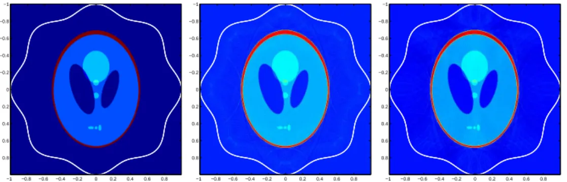
An interesting problem in imaging is to model and compensate for the ef-fects of wave attenuation on image quality. Most imaging techniques either em-phasize a non-attenuating medium or do not adequately incorporate underly-ing phenomenon in reconstruction algorithms. As a consequence, one retrieves erroneous or less accurate wave synthetics which produce serious blurring in reconstructed images (see, for example, Figures 0.1, 0.2 and 0.3 ) and result in loss of important information [86, 109, 132, 134].

The envisaged problem is indeed challenging and has received consider-ably less attention because of its inherent mathematical difficulty. In fact, only recently, some efforts have been made to establish realistic models for wave propagation in attenuating media and a handful of imaging algorithms are pro-posed which compensate for attenuation effects. (See for instance, survey arti-cles [82, 133]. See also [41, 86, 104, 132, 134] and references therein). This

stantiates a real need to investigate attenuation effect on image quality and to propose its remedies for image reconstruction.

This thesis is devoted to study attenuation and to develop stable and robust algorithms for reconstructing acoustic and elastic sources in attenuating media. The source localization problems have been of significant interest in recent years and find numerous applications in different fields, particularly in biomedical imaging [11, 19, 67, 79, 106, 117, 122, 130]. Our main motivation is the recent advances on hybrid ensemble methods making use of elastic and acoustic prop-erties of soft tissues [11, 19, 20, 71, 113]. We also address the problem of locating ambient noise sources in attenuating media [29, 67, 68, 69, 112].

−1 −0.8 −0.6 −0.4 −0.2 0 0.2 0.4 0.6 0.8 −1 −0.8 −0.6 −0.4 −0.2 0 0.2 0.4 0.6 0.8 −1 −0.8 −0.6 −0.4 −0.2 0 0.2 0.4 0.6 0.8 −1 −0.8 −0.6 −0.4 −0.2 0 0.2 0.4 0.6 0.8 −1 −0.8 −0.6 −0.4 −0.2 0 0.2 0.4 0.6 0.8 −1 −0.8 −0.6 −0.4 −0.2 0 0.2 0.4 0.6 0.8 −1 −0.8 −0.6 −0.4 −0.2 0 0.2 0.4 0.6 0.8 −1 −0.8 −0.6 −0.4 −0.2 0 0.2 0.4 0.6 0.8 −1 −0.8 −0.6 −0.4 −0.2 0 0.2 0.4 0.6 0.8 −1 −0.8 −0.6 −0.4 −0.2 0 0.2 0.4 0.6 0.8 −1 −0.8 −0.6 −0.4 −0.2 0 0.2 0.4 0.6 0.8 −1 −0.8 −0.6 −0.4 −0.2 0 0.2 0.4 0.6 0.8

FIGURE0.1. Image reconstruction using elastic time reversal algorithm: First row: Pressure

Component; Second Row: Shear Component. Left to right: initial sources, reconstruction in a loss-less medium, reconstruction in an attenuating medium.

−1 −0.8 −0.6 −0.4 −0.2 0 0.2 0.4 0.6 0.8 −1 −0.8 −0.6 −0.4 −0.2 0 0.2 0.4 0.6 0.8 −1 −0.8 −0.6 −0.4 −0.2 0 0.2 0.4 0.6 0.8 −1 −0.8 −0.6 −0.4 −0.2 0 0.2 0.4 0.6 0.8 −1 −0.8 −0.6 −0.4 −0.2 0 0.2 0.4 0.6 0.8 −1 −0.8 −0.6 −0.4 −0.2 0 0.2 0.4 0.6 0.8 0 0.1 0.2 0.3 0.4 0.5 0.6 0.7 0.8 0.9 1

FIGURE0.2. Image reconstruction using acoustic time reversal algorithm: Left to right: initial

50 100 150 200 250 50 100 150 200 250 50 100 150 200 250 50 100 150 200 250 50 100 150 200 250 50 100 150 200 250

FIGURE0.3. Reconstruction of acoustic sources using Radon transform: Left to right: initial

source; reconstruction in a loss-less medium; reconstruction in an attenuating medium.

M

In this section, we briefly introduce the set of problems under consideration in mathematical context and summarize important results of the thesis.

STATEMENT OF THE PROBLEMS STUDIED

Letpbe the solution of the wave equation

     1 c2 ∂2_p ∂t2(x, t ) − ∆p(x, t) = 0, (x, t ) ∈ R d × R+, p(x, 0) = p0(x) and ∂p ∂t(x, 0) = 0, (1)

where c is the phase velocity and the support, supp©p0(x)ª, of p0(x)is strictly contained in a bounded domainΩ ⊂ Rdwithd = 2,3. Then, the problem(Pi d eal), defined as (Pi d eal) ¯ ¯ ¯ ¯ ¯

reconstructp0(x)given the measurements

n

g (y, t ) := p(y, t), ∀(y, t ) ∈ ∂Ω × (0, T )oforT sufficiently large,

is tractable. Indeed,(Pi d eal)can be related to the spherical Radon transform

R £f ¤(y,r ) =

ˆ Sd −1

rd −1f (y + r ξ)dσ(ξ) (2)

where dσ is the standard surface measure on the unit sphere Sd −1 in Rd_{. A} large class of retro-projection inversion formulae exists for R. Several other techniques such as time reversal, spectral decomposition and optimal control can also be applied [37, 60, 61, 73, 74, 85, 99].

A major drawback of problem(Pi d eal) is that it does not take into account the inevitable frequency dependent wave attenuation severely affecting high frequency components in measured data. This proves to be an impediment to imaging sharp edges and small structures, which correspond to the short wave-lengths and therefore to the high frequencies, thereby introducing blur in images and causing loss of information.

In order to account for wave attenuation, we consider the problem (Pat t) defined as (Pat t) ¯ ¯ ¯ ¯ ¯

reconstructp0(x)given the measurements

n

ga(y, t ) := pa(y, t ), ∀(y, t ) ∈ ∂Ω × (0, T )

o

forT sufficiently large,

wherepa is the solution of the attenuated wave equation:

1 c2 ∂2_p a ∂t2 (x, t ) − ∆pa(x, t ) − La£pa¤ (x, t) = 0, (x, t) ∈ R d × R+ (3) with loss operatorLa. In contrast with (Pi d eal), the problem(Pat t)is more in-volved and intricate. Indeed, it is quite troublesome to adopt ideal reconstruc-tion algorithms to solve(Pat t) because attenuation induces instability. On the other hand, some of the algorithms even fail as their underlying assumptions are no more valid. For example, the ideal time reversal technique does not work be-cause attenuation breaks down the time reversibility of waves. A further prob-lematic situation is when we have to impose boundary condition onpa or have access to only partial boundary dataga.

The viscoelastic counterpart of(Pat t), that is,

(Pve) ¯ ¯ ¯ ¯ ¯

reconstructu0(x)given the measurements

n

ga(y, t ) := ua(y, t ), ∀(y, t ) ∈ ∂Ω × (0, T )

o

forT sufficiently large,

is even more challenging and hard-won whereusatisfies viscoelastic wave equa-tion: µ ρ∂2 ∂t2− Lλ,µ− ∂ ∂tLηλ,ηµ ¶ ua(x, t ) =∂δ0 (t ) ∂t u0(x), (x, t ) ∈ R d × R+, (4) with Lamé parameters(λ,µ), viscoelastic moduli(η_λ,η_µ)and

La,bv = (a + b)∇(∇ · v) − b∆v.

The additional difficulty in(Pve)stems from the fact that the measured data is a combination of both shear and pressure waves having different phase velocities and polarization directions.

In this thesis, we aim to present stable and robust algorithms in order to solve(Pat t),(Pve)and the allied problems. We also address their applications to biomedical imaging and ambient noise imaging.

SUMMARY OF THE MAIN RESULTS

First of all, we consider Radon transform based algorithms to solve(Pat t). For simplicity, we letpasatisfy thermo-viscous wave equation:

1 c2 ∂2_p a ∂t2 (x, t ) − ∆pa(x, t ) − a ∂ ∂t ¡ ∆pa¢ (x, t) = 0, (x, t) ∈ Rd× R+ (5)

where a represents attenuation coefficient. Whena is constant, we relate non-attenuated waveptopa via an attenuation operatorL as

pa= L£p¤, where L £φ¤(x,t) =p1 2π ˆ R ˆ R+ 1 p 1 + i aωφ(x,s)exp ½ _iωs p 1 + i aω ¾ exp©iωtªdsdω. (6)

The attenuation correction can be achieved by inverting L. However, L is ill-conditioned. Therefore, by using stationary phase theorem, we present an asymptotic development ofL with respect to a small attenuation coefficienta

of the form L £φ¤ =Xk j =0 ajLk £ φ¤ + o(ak_).

This permits us to find an approximate inverseL−1

k of the attenuation operator and therefore the ideal Radon transform of the initial conditions. Subsequently we findp0(x)using retro-projection inverse Radon transform formulae [60, 61]. We compare our results with a singular value decomposition approach for ap-proximatingL−1_{, as taken in [86, 95]. Our results appear to be more stable and} accurate. The partial boundary data problems are treated with TV-Tikhonov reg-ularization techniques [72]. We study three different iterative algorithms and present special preconditioning weights in order to increase convergence speed. Finally, in the case of imposed boundary conditions, we use a duality approach originally proposed in [11], whereas stationary phase theorem is used to rectify attenuation artifacts. We also explain the case of power-law attenuation correc-tion [82, 127].

Motivated by their simplicity and robustness, we then study the time rever-sal techniques to solve (Pat t) and (Pve) [46, 62]. As the attenuating waves are not time invariant, we test the idea of using adjoint attenuated waves for time reversal, as suggested by [41, 134]. For (Pat t), we justify mathematically us-ing attenuation operatorL previously defined, that this technique provides an approximation ofp0correct up to first order of attenuation, but it is not quite sta-ble. As an alternative we propose a preprocessing technique consisting of two steps: use asymptotically obtained filterL_k−1to pre-process measured data and afterward an ideal time reversal algorithm. We establish that the new technique is more stable and is accurate up to orderk.

The elastic time reversal is studied for both elastic and viscoelastic media. In elastic media, the boundary data

©g(y, t) := u(y, t), (y, t) ∈ Rd

× (0, T )ª

is a combination of the pressure and the shear waves propagating with different phase velocities and polarization directions. Consequently, we observe addi-tional artefacts when we time reverse the displacement field. Therefore, we first

address these artefacts by proposing an original technique based on a weighted Helmholtz decomposition. Then, we solve (Pve) using a regularized version of adjoint viscoelastic wave together with modified time reversal functional. We prove that our results are of order(ν2s/cs2+ν2p/cp2), where(νs,νp)are the shear and bulk viscosities and(cs, cp)are the shear and pressure wave speeds respectively. As an application of the inverse source problems, we aim to locate noise sources from boundary measurements over an interval of time. More precisely, we consider the following problem:

(Pnoi se) ¯ ¯ ¯ ¯ ¯

reconstruct spatial supportK (x)of noise sourcen(x, t )given

n

g (y, t ) := p(y, t), ∀(y, t ) ∈ ∂Ω × (0, T )

o

forT sufficiently large,

wherepis the solution of the wave equation (1) ( respectively (3) for attenuating media) with sourcen(x, t )being a stationary Gaussian process with mean zero and covariance function

〈n(t , x)n(s, y)〉 = F (t − s)K (x)δ(x − y).

HereFis the time covariance of the noise signals and〈·〉stands for the statistical average. By using statistical cross correlation of the noise signals, we propose efficient weighted functionals to solve (Pnoi se), with and without attenuation. In attenuating media, we use a regularized version of the back-propagator to locate sources. We also discuss the impact of spatial correlation between the noise sources and derive functionals capable of first locating such sources and then estimating their correlation matrix.

In another study, we adopt the ideal anomaly detection algorithms to the case of a quasi-incompressible viscoelastic medium. For doing so, we first derive a closed form expression of the viscoelastic Green function in a homogeneous isotropic medium. We show that when the compressional modulusλ → ∞the ideal elastic Green function, Gi d eal, can be approximated from the viscoelastic Green function, Gat t, by solving an ordinary differential equation. This result is also based on the asymptotic development of an attenuation operator using stationary phase theorem.

Finally, we provide some anisotropic viscoelastic Green functions with an aim to enhance our results to the case of anisotropic media. We follow an ap-proach proposed by Burridge et al. [42]. We write Green function in terms of three functions, φi, satisfying the scalar wave equation in attenuating media. The problem of finding the Green function is then related to resolve the wave equations in order to findφi’s and three subsequent potential equations of the form

∆Eψi= φi,

where∆E is the Laplacian in ellipsoidal coordinates. The potential equation is finally solved using an argument of potential theory in ellipsoidal coordinates [50, 80].

T

The thesis consists of six chapters, essentially divided into two parts.

PART I deals with imaging techniques in acoustic media and their applica-tions to biomedical imaging and noise source imaging. It consists of CHAPTERS

1, 2 and 3.

CHAPTER 1 is devoted to the reconstruction algorithms based on Radon

transform and their applications to Photoacoustic imaging in attenuating media. We detail results related to attenuation correction, imposed boundary conditions and partial data problems.

CHAPTER2 presents time reversal methods to find acoustic sources. We

re-call time reversal techniques for ideal acoustic media and analyze the technique based on an adjoint attenuated wave. Finally, we provide an algorithm based on pre-processing of the measured data.

CHAPTER 3 deals with the problems of locating ambient noise sources in

acoustic media. We present algorithms to locate point as well as extended sources in both attenuating and non-attenuating media. The case of spatially correlated sources is also discussed.

PART IIdeals with imaging in elastic media and consists of CHAPTERS 4, 5

and 6.

CHAPTER4 addresses the imaging problems in isotropic viscoelastic media

in a quasi-incompressible regime. We first present an expression for viscoelastic Green function and then provide a stable technique for attenuation correction.

CHAPTER5 aims to present and justify the time reversal techniques for

vis-coelastic media. We discuss a modified time reversal functional in a purely elas-tic regime to tackle imaging artefacts. Then, we extend this technique to vis-coelastic media.

CHAPTER6 deals with visco-elastic anisotropy in order to extend results

pre-sented in Chapter 4 and 5.

Finally, we sum up the thesis in CONCLUSION AND PERSPECTIVES, where

we also discuss some open questions related to the subject matter.

All the chapters of the thesis are self-contained and can be read indepen-dently. Thesis mainly contains the results presented in [14, 15, 16, 17, 39, 40].

Part I

Imaging in Attenuating Acoustic

Media

C

H

A

P

T

1

P

-

I

A

M

1.1

I

In photo-acoustic imaging, optical energy absorption causes thermo-elastic ex-pansion of the tissue, which leads to the propagation of a pressure wave. This signal is measured by transducers distributed on the boundary of the object, which in turn is used for imaging optical properties of the object. The major contribution of photo-acoustic imaging is to provide images of optical contrasts (based on the optical absorption) with the resolution of ultrasound [145].

If the medium is acoustically homogeneous and has the same acoustic prop-erties as the free space, then the boundary of the object plays no role and the optical properties of the medium can be extracted from measurements of the pressure wave by inverting a spherical Radon transform [73, 74, 84].

If a boundary condition has to be imposed on the pressure field, then an ex-plicit inversion formula no longer exists. However, using a quite simple duality approach, one can still reconstruct the optical absorption coefficient. In fact, in the recent works [11, 12], Ammari et al. investigated quantitative photoacoustic imaging in the case of a bounded medium with imposed boundary conditions. In a further study [10], they proposed a geometric-control approach to deal with the case of limited view measurements. In both cases, they focused on a situa-tion with small optical absorbers in a non-absorbing background and proposed adapted algorithms to locate the absorbers and estimate their absorbed energy.

A second challenging problem in photo-acoustic imaging is to take into ac-count the issue of modeling the acoustic attenuation and its compensation. This subject is addressed in [41, 81, 83, 86, 92, 104, 124, 132].

In this chapter, we propose a new approach to image extended optical sources from photo-acoustic data and to correct the effect of acoustic attenuation. By testing our measurements against an appropriate family of functions, we show that we can access the Radon transform of the initial condition, and thus recover quantitatively any initial condition for the photoacoustic problem. We also show

how to compensate the effect of acoustic attenuation on image quality by using the stationary phase theorem. We use a frequency power-law model for the at-tenuation losses.

The chapter is organized as follows. In Section 1.2 we consider the photo-acoustic imaging problem in free space. We first propose three algorithms to re-cover the absorbing energy density from limited-view and compare their speeds of convergence. We then present two approaches to correct the effect of acoustic attenuation. We use a power-law model for the attenuation. We test the singular value decomposition approach proposed in [86] and provide a new technique based on the stationary phase theorem. Section 1.3 is devoted to correct the ef-fect of imposed boundary conditions. By testing our measurements against an appropriate family of functions, we show how to obtain the Radon transform of the initial condition in the acoustic wave equation, and thus recover quantita-tively the absorbing energy density. We also show how to compensate for the effect of acoustic attenuation on image quality by once again using the station-ary phase theorem. The chapter ends with a discussion.

1.2

P

-

In this section, we first formulate the imaging problem in free space and present a simulation for the reconstruction of the absorbing energy density using the spherical Radon transform. Then, we provide a total variation regularization to find a satisfactory solution of the imaging problem with limited-view data. Finally, we present two deconvolution strategies to compensate for the effect of acoustic attenuation and compare their performance. The first strategy is based on a singular value decomposition while the second one uses the station-ary phase theorem.

1.2.1 MATHEMATICAL FORMULATION

We consider the wave equation inRd,

1 c₀2 ∂2_p ∂t2(x, t ) − ∆p(x, t) = 0 in R d × (0, T ), with p(x, 0) = p0 and ∂p ∂t(x, 0) = 0.

Herec0is the phase velocity in a non-attenuating medium.

Assume that the support ofp0, the absorbing energy density, is contained in a bounded setΩ ofRd. Our objective in this part is to reconstruct p0 from the measurements

n

where∂Ωdenotes the boundary ofΩ.

The problem of reconstructingp0 is related to the inversion of the spherical Radon transform given by

RΩ£ f ¤(y,r ) = ˆ

S

r f (y + r ξ)dσ(ξ), (y, r ) ∈ ∂Ω × R+,

where S denotes the unit sphere. It is known that in dimension2, Kirchhoff’s formula implies that [61]

         p(y, t ) = 1 2π ∂ ∂t ˆ t 0 RΩ£p0¤ (y,c0r ) p t2_{− r}2 d r, RΩ£p0¤ (y,r ) = 4r ˆ r 0 p(y, t /c0) p r2_{− t}2 d t .

Let the operatorW be defined by

W £g¤(y,r ) = 4r ˆ r 0 g (y, t /c0) p r2_{− t}2 d t for allg :∂Ω × R + → R. (1.1)

Then, it follows that

RΩ£p0¤ (y,r ) = W £p¤(y,r ). (1.2) In recent works, a large class of inversion retro-projection formulae for the spherical Radon transform have been obtained in even and odd dimensions when Ω is a ball; see for instance [60, 61, 85, 99]. In dimension2, when Ω is the unit ball, it turns out that

p0(x) = 1 (4π2₎ ˆ ∂Ω ˆ 2 0 · _d2 d r2RΩ£p0¤ (y,r ) ¸ ln¯¯r2− (y − x)2 ¯ ¯d r dσ(y). (1.3)

This formula can be rewritten as follows:

p0(x) = 1 4π2R ∗ ΩBRΩ£p0¤ (x), whereR∗ Ωis the adjoint ofRΩ, R∗ Ω£g ¤(x) = ˆ ∂Ωg (y, |y − x|)dσ(y), andBis defined by B £g¤(x,t) = ˆ 2 0 d2g d r2(y, r ) ln ¯ ¯r2− t2 ¯ ¯d r forg :Ω × R+→ R.

In Figure 1.1, we give a numerical illustration for the reconstruction of p0 using the spherical Radon transform. We adopt the same approach as in [60] for the discretization of formulae (1.1) and (1.3).

50 100 150 200 250 50 100 150 200 250 20 40 60 80 100 120 140 160 180 200 20 40 60 80 100 120 140 160 180 200 20 40 60 80 100 120 140 160 180 200 20 40 60 80 100 120 140 160 180 200 50 100 150 200 250 50 100 150 200 250

FIGURE1.1. Numerical inversion using(1.3) withN = 256,NR= 200andNθ= 200. Top left:

p0; Top right:p(y, t )with(y, t ) ∈ ∂Ω × (0,2); Bottom left:RΩ£p0¤ (y, t)with(y, t ) ∈ ∂Ω × (0,2);

Bottom right: 1

4π2R∗_ΩBRΩ£p0

¤

.

1.2.2 LIMITED-VIEW DATA

In many situations, we have only at our disposal data onΓ×(0,T ), whereΓ ⊂ ∂Ω. As illustrated in Figure 1.2, restricting the integration in formula (1.3) to Γ as follows: p0(x) ' 1 (4π2₎ ˆ Γ ˆ 2 0 ·_d2 d r2RΩ£p0¤ (y,r ) ¸ ln¯¯r2− (y − x)2 ¯ ¯d r dσ(y), (1.4)

is not stable enough to give a correct reconstruction ofp0.

The inverse problem becomes severely ill-posed and needs to be regularized; see for instance [72, 146]. We apply here a Tikhonov regularization with a total variation term, which is well adapted to the reconstruction of smooth solutions with front discontinuities. We then introduce the functionp0,ηas the minimizer of J [ f ] =°° °Q £ RΩ£ f ¤ − g ¤ ° ° °_L2_{(∂Ω×(0,2))}+ η ° °∇ f ° °_L1_(Ω),

whereQ is a positive weight operator.

Direct computation ofp0,ηcan be complicated as the TV term is not smooth (not of class C1). Here, we obtain an approximation of p0,η via an iterative

−1 −0.8 −0.6 −0.4 −0.2 0 0.2 0.4 0.6 0.8 1 −1 −0.8 −0.6 −0.4 −0.2 0 0.2 0.4 0.6 0.8 1 0 0.1 0.2 0.3 0.4 0.5 0.6 0.7 0.8 0.9 1 −1 −0.8 −0.6 −0.4 −0.2 0 0.2 0.4 0.6 0.8 1 −1 −0.8 −0.6 −0.4 −0.2 0 0.2 0.4 0.6 0.8 1 −0.2 0 0.2 0.4 0.6 0.8 1

FIGURE 1.2. Numerical inversion with truncated(1.3) formula. N = 128, NR= 128, and

N_{θ= 30}. Left:p0; Right: ₄1_π2R∗_ΩBRΩ£p0¤.

shrinkage-thresholding algorithm [52, 55]. This algorithm can be seen as a split, gradient-descent, iterative scheme:

• Datag, initial solution f0= 0;

• (1) Data link step: f_k+1/2= fk− γR∗_ΩQ∗Q

£

RΩ£ fk¤ − g ¤; • (2) Regularization step: fk= Tγη£ fk+1/2

¤

,

whereγis a virtual descent time step and the operatorTηis defined by

T_η[y] = ar g min x n_° °y − x ° °_L2+ η k∇xkL1 o .

One advantage of the algorithm is to minimize implicitly the TV term using the duality algorithm of Chambolle [49]. This algorithm converges [52, 55] under the assumption γ°°R∗

ΩQ∗QRΩ

°

°≤ 1, but its rate of convergence is known to be

slow. Thus, in order to accelerate the convergence rate, we will also consider a variant algorithm of Beck and Teboulle [34] defined as

• Datag, initial set: f0= x0= 0,t1= 1; • (1)xk= Tγη ³ fk− γR_Ω∗Q∗Q £ RΩ£ fk¤ − g ¤ ´ ; • (2) f_k+1= xk+ tk− 1 t_k+1 (xk− xk−1) with tk+1= 1 +q1 + 4t_k2 2 .

The standard choice ofQ is the identity, Id, and then it is easy to see that

° °RΩR∗_Ω

°

°' 2π. It will be also interesting to useQ =₂1_πB1/2, which is well defined

sinceBis symmetric and positive. In this case,R∗

ΩQ∗Q ' R−1Ω and we can hope

−1 −0.8 −0.6 −0.4 −0.2 0 0.2 0.4 0.6 0.8 1 −1 −0.8 −0.6 −0.4 −0.2 0 0.2 0.4 0.6 0.8 1 −0.1 0 0.1 0.2 0.3 0.4 0.5 0.6 0.7 0.8 −1 −0.8 −0.6 −0.4 −0.2 0 0.2 0.4 0.6 0.8 1 −1 −0.8 −0.6 −0.4 −0.2 0 0.2 0.4 0.6 0.8 1 −0.2 0 0.2 0.4 0.6 0.8 1 −1 −0.8 −0.6 −0.4 −0.2 0 0.2 0.4 0.6 0.8 1 −1 −0.8 −0.6 −0.4 −0.2 0 0.2 0.4 0.6 0.8 1 0 0.1 0.2 0.3 0.4 0.5 0.6 0.7 0.8 0.9 1 0 5 10 15 20 25 30 35 40 45 50 0.05 0.1 0.15 0.2 0.25 0.3 0.35 0.4 0.45 0.5 0.55 methode 1 methode 2 methode3

FIGURE1.3. Iterative shrinkage-thresholding solution after30iterations withη = 0.01,N =

128,NR= 128, andN_θ= 30. Top left: simplest algorithm withQ = Id andµ = 1/(2π); Top right:

simplest algorithm withQ =21πB1/2andµ = 0.5; Bottom left: Beck and Teboulle variant with

Q =₂1_πB1/2andµ = 0.5; Bottom right: errork → kfk− p0k∞for each of the previous situations.

We compare three algorithms of this kind in Figure 1.3. The first and the second one correspond to the simplest algorithm with Q = Id andQ = 21πB1/2 respectively. The last method uses the variant of Beck and Teboulle with Q =

1 2πB

1/2_{.The speed of convergence for each one of these algorithms is presented} in Figure 1.3. Clearly, the third method is the best and after30iterations, a very good approximation ofp0is reconstructed.

Two limited-angle experiments are presented in Figure 1.4 using the third algorithm.

1.2.3 COMPENSATION OF THE EFFECT OF ACOUSTIC ATTENUATION

Our aim in this section is to compensate for the effect of acoustic attenuation. The pressuresp(x, t )andpa(x, t )are respectively solutions of the following wave equations: 1 c2₀ ∂2_p ∂t2(x, t ) − ∆p(x, t) = 1 c₀2 ∂ ∂tδt =0p0(x),

−1 −0.8 −0.6 −0.4 −0.2 0 0.2 0.4 0.6 0.8 1 −1 −0.8 −0.6 −0.4 −0.2 0 0.2 0.4 0.6 0.8 1 0 0.1 0.2 0.3 0.4 0.5 0.6 0.7 0.8 0.9 1 −1 −0.8 −0.6 −0.4 −0.2 0 0.2 0.4 0.6 0.8 1 −1 −0.8 −0.6 −0.4 −0.2 0 0.2 0.4 0.6 0.8 1 0 0.1 0.2 0.3 0.4 0.5 0.6 0.7 0.8 0.9 1 −1 −0.8 −0.6 −0.4 −0.2 0 0.2 0.4 0.6 0.8 1 −1 −0.8 −0.6 −0.4 −0.2 0 0.2 0.4 0.6 0.8 1 −0.2 0 0.2 0.4 0.6 0.8 1 1.2 −1 −0.8 −0.6 −0.4 −0.2 0 0.2 0.4 0.6 0.8 1 −1 −0.8 −0.6 −0.4 −0.2 0 0.2 0.4 0.6 0.8 1 −0.4 −0.2 0 0.2 0.4 0.6 0.8 1 1.2 −1 −0.8 −0.6 −0.4 −0.2 0 0.2 0.4 0.6 0.8 1 −1 −0.8 −0.6 −0.4 −0.2 0 0.2 0.4 0.6 0.8 1 0 0.1 0.2 0.3 0.4 0.5 0.6 0.7 0.8 0.9 1 −1 −0.8 −0.6 −0.4 −0.2 0 0.2 0.4 0.6 0.8 1 −1 −0.8 −0.6 −0.4 −0.2 0 0.2 0.4 0.6 0.8 1 0 0.2 0.4 0.6 0.8 1 1.2

FIGURE1.4. Limited angle case with Beck and Teboulle iterative shrinkage-thresholding after

50iterations, with parameters:η = 0.01,N = 128,NR= 128,N_θ= 64andQ =

1 2πB 1/2_{. Top to} Bottom:p0; 1 4π2R∗ΩBRΩ£p0 ¤

and 1 c₀2 ∂2_p a ∂t2 (x, t ) − ∆pa(x, t ) − L(t) ∗ pa(x, t ) = 1 c2₀ ∂ ∂tδt =0p0(x), whereLis defined by L(t ) =p1 2π ˆ R Ã κ2 (ω) −ω 2 c₀2 ! eiωtdω. (1.5)

Many models exist forκ(ω)[82]. Here we use the power-law model. Thenκ(ω) is the complex wave number, defined by

κ(ω) = ω

c(ω)+ i a|ω|

ζ_{, (1.6)}

where ω is the frequency, c(ω) is the frequency dependent phase velocity and

1 ≤ ζ ≤ 2 is the power-law exponent; see [83, 125]. A common model, known as the thermo-viscous model, is given byκ(ω) = ω

c0p1 − i aωc0

and corresponds approximately toζ = 2withc(ω) = c0.

Our strategy is now to:

• Estimatep(y, t )frompa(y, t )for all(y, t ) ∈ ∂Ω × R+.

• Apply the inverse formula for the spherical Radon transform to recon-structp0from the non-attenuated data.

A natural definition of an attenuated spherical Radon transformRΩ,ais

RΩ,a£p0¤ = W £pa¤ .

1.2.4 RELATIONSHIP BETWEENp ANDpa

Recall that the Fourier transforms ofp andpa satisfy

µ ∆ + µω c0 ¶2¶ b p(x,ω) =piω 2πc2₀p0(x) and ¡ ∆ + κ(ω)2¢ b pa(x,ω) = iω p 2πc2₀p0(x),

which implies that

b

p¡x,c0κ(ω)¢ =

c0κ(ω)

ω pba(x,ω).

The issue is to estimatepfrompa using the relationshippa= L£p¤, whereL is defined by L £φ¤(s) = 1 2π ˆ R ω c0κ(ω) e−i ωs ˆ _∞ 0 φ(t)exp©ic 0κ(ω)tªdt dω.

50 100 150 200 250 50 100 150 200 250 20 40 60 80 100 120 140 160 180 200 20 40 60 80 100 120 140 160 180 200 20 40 60 80 100 120 140 160 180 200 20 40 60 80 100 120 140 160 180 200 50 100 150 200 250 50 100 150 200 250

FIGURE1.5. Numerical inversion of attenuated wave equation withκ(ω) =ω

c0+i a

ω2

2 anda =

0.001. HereN = 256,NR= 200andNθ= 200. Top left:p0; Top right:pa(y, t )with(y, t ) ∈ ∂Ω ×

(0, 2); Bottom left:W £pa¤ (y, t)with(y, t ) ∈ ∂Ω × (0,2); Bottom right:

1

4π2R∗ΩB¡W £pa¤ (y, t)¢.

The main difficulty is that L is not well conditioned. We will compare two approaches. The first one uses a regularized inverse of L via a singular value decomposition (SVD), which has been recently introduced in [86]. The second one is based on the asymptotic behavior of L as the attenuation coefficient a

tends to zero.

Figure 1.5 gives some numerical illustrations of the inversion of the atten-uated spherical Radon transform without a correction of the attenuation effect, where a thermo-viscous attenuation model is used withc0= 1.

1.2.5 ASINGULAR VALUE DECOMPOSITION APPROACH

La Rivière, Zhang and Anastasio have recently proposed in [86] to use a regu-larized inverse of the operatorL obtained by a standard SVD approach:

L £φ¤ = X

l

where (ψel) and(ψl) are two orthonormal bases ofL

2_{(0, T )andσ}

l are positives eigenvalues such that

             L∗£ φ¤ =P lσl〈φ, ψl〉ψel, L∗_{L £φ¤ = P} lσ2_l〈φ,ψel〉ψel, L L∗£ φ¤ = Plσ2_l〈φ, ψl〉ψl.

An²-approximation inverse ofL is then given by

L−1 1,² £ φ¤ = X l σl σ2 l + ²2 〈φ, ψl〉ψel, where² > 0.

In Figure 1.6 we present some numerical inversions of the thermo-viscous wave equation with a = 0.0005 anda = 0.0025. We first obtain the ideal mea-surements from the attenuated ones and then apply the inverse formula for the spherical Radon transform to reconstruct p0from the ideal data. We take ² re-spectively equal to0.01,0.001and0.0001. As expected, this algorithm corrects a part of the attenuation effect but is unstable when²tends to zero.

1.2.6 ASYMPTOTICS OFL

In physical situations, the coefficient of attenuationais very small. We will take this phenomenon into account and introduce an approximation of L andL−1 asagoes to zero: Lk£φ¤ = L £φ¤ + o ³ ak+1´ and L−1 2,k £ φ¤ = L−1£ φ¤ + o³ak+1´,

wherek represents an order of approximation.

1.2.6.1 THERMO-VISCOUS CASE:κ(ω) ' ω

c0+ i a

ω2

2

Let us consider in this section the attenuation model κ(ω) ' ω

c0+ i a ω2 2 at low frequenciesω ¿ 1 a, such that 1 1 + i ac0ω/2' 1 − i ac0 2 ω.

The operatorL is approximated as follows

L £φ¤(s) ' 1 2π ˆ _∞ 0 φ(t) ˆ R ³ 1 − iac0 2 ω ´ exp ½ −1 2c0aω 2_t¾_{exp©iω(t − s)ªdωdt.}

50 100 150 200 250 50 100 150 200 250 0 0.1 0.2 0.3 0.4 0.5 0.6 0.7 0.8 0.9 1 50 100 150 200 250 50 100 150 200 250 0 0.1 0.2 0.3 0.4 0.5 0.6 0.7 50 100 150 200 250 50 100 150 200 250 0 0.1 0.2 0.3 0.4 0.5 0.6 0.7 0.8 0.9 1 50 100 150 200 250 50 100 150 200 250 0 0.1 0.2 0.3 0.4 0.5 0.6 0.7 0.8 50 100 150 200 250 50 100 150 200 250 0 0.1 0.2 0.3 0.4 0.5 0.6 0.7 0.8 0.9 1 50 100 150 200 250 50 100 150 200 250 0 0.1 0.2 0.3 0.4 0.5 0.6 0.7 0.8 0.9 1

FIGURE1.6. Compensation of acoustic attenuation with SVD regularization: N = 256,NR=

200and N_{θ= 200}. Left: a = 0.0005; Right: a = 0.0025. Top to bottom: L−1

1,² with² = 0.01,

Since 1 p 2π ˆ Rexp ½ −1 2c0aω 2_t¾_{exp©iω(t − s)ªdω =} 1 p c0at exp ½ −1 2 (s − t)2 c0at ¾ , and 1 p 2π ˆ R −i ac0ω 2 exp ½ −1 2c0aω 2_t¾_{exp©iω(t−s)ªdω =}ac0 2 ∂ ∂s µ ₁ p c0at exp ½ −1 2 (s − t)2 c0at ¾¶ , it follows that L £φ¤ ' µ 1 +ac0 2 ∂ ∂s ¶ µ ₁ p 2π ˆ _+∞ 0 φ(t)p1 c0at exp ½ −1 2 (s − t)2 c0at ¾ d t ¶ .

We then investigate the asymptotic behavior ofLfdefined by f L £φ¤ =p1 2π ˆ _+∞ 0 φ(t) 1 p c0at exp ½ −1 2 (s − t)2 c0at ¾ d t . (1.7)

Since the phase in (1.7) is quadratic anda is small, by the stationary phase theo-rem we can prove that

f L £φ¤(s) =Xk i =0 (c0a)i 2i_{i !} Di £ φ¤(s) + o³ak´, (1.8)

where the differential operatorsDisatisfyDi£φ¤(s) = (tiφ(t))(2i )(s); see Appendix 1.A.2. We can also deduce the following approximation of orderkofLf−1

f L−1 k £ ψ¤ =Xk j =0 ajψk, j, (1.9)

whereψk, j are defined recursively by

ψk,0= ψ and ψk, j= − j X i =1 c₀i 2i_{i !}Di £

ψk, j −i¤ , for allj ≤ k. Finally, we define Lk= µ 1 +ac0 2 ∂ ∂s ¶ f Lk and L2,k−1= fLk−1 µ 1 +ac0 2 ∂ ∂t ¶−1 . (1.10)

We present in Figure 1.7 some numerical reconstructions ofp0using a thermo-viscous wave equation with a = 0.0005 and a = 0.0025. We take respectively:

k = 0, k = 1 andk = 8. These reconstructions seem to be as good as those

ob-tained by the SVD regularization approach. Moreover, this new algorithm has better stability properties.

50 100 150 200 250 50 100 150 200 250 0 0.1 0.2 0.3 0.4 0.5 0.6 50 100 150 200 250 50 100 150 200 250 0 0.05 0.1 0.15 0.2 0.25 0.3 0.35 0.4 50 100 150 200 250 50 100 150 200 250 0 0.1 0.2 0.3 0.4 0.5 0.6 0.7 0.8 50 100 150 200 250 50 100 150 200 250 0 0.05 0.1 0.15 0.2 0.25 0.3 0.35 0.4 0.45 0.5 50 100 150 200 250 50 100 150 200 250 0 0.1 0.2 0.3 0.4 0.5 0.6 0.7 0.8 0.9 1 50 100 150 200 250 50 100 150 200 250 0 0.1 0.2 0.3 0.4 0.5 0.6 0.7 0.8

FIGURE1.7. Compensation of acoustic attenuation with formula(1.10): N = 256,NR= 200

andN_{θ= 200}. Left:a = 0.0005; Right: a = 0.0025. Top to Bottom: Lf−1

k withk = 0;k = 1and

1.2.6.2 GENERAL CASE:κ(ω) = ω

c0+ i a|ω|

ζ_{WITH1 ≤ ζ < 2}

We now consider the attenuation model κ(ω) = ω

c0+ i a|ω|

ζ _{with 1 ≤ ζ < 2. As} before, this problem can be reduced to the approximation of the operator Lf

defined by f L £φ¤(s) = ˆ _∞ 0 φ(t) ˆ Rexp©iω(t − s)ªexp© − |ω| ζ_c 0atª dωdt. It is also interesting to see that its adjointLf∗satisfies

f L∗£ φ¤(s) = ˆ _∞ 0 φ(t) ˆ Rexp©iω(s − t)ªexp© − |ω| ζ_c 0asª dωdt.

Suppose for the moment thatζ = 1, and working with the adjoint operatorL∗_, we see that f L∗£ φ¤(s) = 1 π ˆ _∞ 0 c0as (c0as)2+ (s − t )2φ(t)dt. Invoking the dominated convergence theorem, we have

lim a→0Lf ∗£ φ¤(s) = lim a→0 1 π ˆ _∞ −_ac01 1 1 + y2φ(s + c0a y s)d y = 1 π ˆ _∞ −∞ 1 1 + y2φ(s)d y = φ(s).

More precisely, introducing the fractional Laplacien∆1/2as follows

∆1/2_{φ(s) =} 1 πp.v. ˆ _+∞ −∞ φ(t) − φ(s) (t − s)2 d t , where p.v. stands for the Cauchy principal value, we get

1 a ¡ f L∗£ φ¤(s) − φ(s)¢ = 1 a ˆ _∞ −∞ 1 πc0as 1 1 +³_cs−t_0as´2 ¡ φ(t) − φ(s)¢dt = ˆ _∞ −∞ 1 π c0s (c0as)2+ (s − t )2 ¡ φ(t) − φ(s)¢dt = lim ²→0 ˆ R\[s−²,s+²] 1 π c0s (c0as)2+ (s − t )2 ¡ φ(t) − φ(s)¢dt → lim ²→0 ˆ R\[s−²,s+²] 1 π c0s (s − t)2 ¡ φ(t) − φ(s)¢dt = c0s∆1/2φ(s),

asatends to zero. We therefore deduce that f L∗£ φ¤(s) = φ(s) + c0as∆1/2φ(s) + o(a) and f L £φ¤(s) = φ(s) + c0a∆1/2¡sφ(s)¢ + o(a). Applying exactly the same argument for1 < ζ < 2, we obtain that

f

L £φ¤(s) = φ(s) +Cc0a∆ζ/2¡sφ(s)¢ + o(a), whereC is a constant, depending only onζand∆ζ/2is defined by

∆ζ/2φ(s) = 1 πp.v. ˆ _+∞ −∞ φ(t) − φ(s) (t − s)1+ζ d t .

1.2.7 AN ITERATIVE SHRINKAGE-THRESHOLDING ALGORITHM WITH

CORRECTION OF ATTENUATION

The previous correction of attenuation is not so efficient for a large attenuation coefficient a. In this case, to further enhance the resolution of the reconstruc-tion, we may use again a Tikhonov regularization. LetR−1

Ω,a,kbe an approximate inverse of the attenuated spherical Radon transformRΩ,a:

R−1

Ω,a,k= RΩ−1W L_2,k−1W−1.

Although its convergence is not clear, we will now consider the following itera-tive shrinkage-thresholding algorithm:

• Datag, initial set: f0= x0= 0,t1= 1; • (1)xj= Tγη ³ fj− γR−1_Ω,a,k ¡ RΩ,afj− g ¢´ ; • (2) f_{j +1}= xj+ tj− 1 t_{j +1} ¡xj− xj −1 ¢ with t_{j +1}= 1 +q1 + 4t2_j 2 .

Figure 1.8 shows the efficiency of this algorithm.

1.3

P

-

-ARY CONDITIONS

In this section, we consider the case where a boundary condition has to be im-posed on the pressure field. We first formulate the photo-acoustic imaging prob-lem in a bounded domain before reviewing the reconstruction procedures. We refer the reader to [140] where the half-space problem has been considered. We then introduce a new algorithm which reduces the reconstruction problem to the

50 100 150 200 250 50 100 150 200 250 0 0.1 0.2 0.3 0.4 0.5 0.6 0.7 0.8 0.9 1 50 100 150 200 250 50 100 150 200 250 0 0.1 0.2 0.3 0.4 0.5 0.6 0.7 0.8 0.9 1 50 100 150 200 250 50 100 150 200 250 0 0.1 0.2 0.3 0.4 0.5 0.6 0.7 0.8 0.9 1 0 10 20 30 40 50 60 0.35 0.4 0.45 0.5 0.55 0.6 0.65 0.7 k = 0 k = 1 k = 4 k = 6

FIGURE1.8. Numerical results for iterative shrinkage-thresholding algorithm withη = 0.001

anda = 0.0025. Left up: f50withk = 0; Top right: f50withk = 1; Bottom left: f50withk = 6;

Bottom right: errorj → kfj− p0kfor different values ofk.

inversion of a Radon transform. This procedure is particularly well-suited for extended absorbers. Finally, we discuss the issue of correcting the attenuation effect and propose an algorithm analogous to the one described in the previous section.

1.3.1 MATHEMATICAL FORMULATION

LetΩbe a bounded domain. We consider the wave equation in the domainΩ:

                 1 c2₀ ∂2_p ∂t2(x, t ) − ∆p(x, t) = 0 in Ω × (0,T ), p(x, 0) = p0(x) inΩ, ∂p ∂t(x, 0) = 0 inΩ, (1.11)

with the Dirichlet (resp. the Neumann) imposed boundary conditions:

p(x, t ) = 0 µ resp. ∂p ∂ν(x, t ) = 0 ¶ on∂Ω × (0,T ). (1.12)

Our objective in the next subsection is to reconstructp0(x)from the measure-ments of ∂p

∂ν(x, t )(resp.p(x, t )) on the boundary∂Ω × (0,T ).

1.3.2 INVERSION ALGORITHMS

Consider probe functions satisfying

                 1 c₀2 ∂2_v ∂t2(x, t ) − ∆v(x, t) = 0 in Ω × (0,T ), v(x, T ) = 0 inΩ, ∂v ∂t(x, T ) = 0 inΩ. (1.13)

Multiplying (1.11) byvand integrating by parts yields (in the case of Dirich-let boundary conditions):

ˆ T 0 ˆ ∂Ω ∂p ∂ν(x, t )v(x, t )dσ(x)dt = ˆ Ωp0(x) ∂v ∂t(x, 0)d x. (1.14)

Choosing a probe functionvwith proper initial time derivative allows us to infer information onp0(right-hand side in (1.14)) from our boundary measure-ments (left-hand side in (1.14)).

In [11], considering a full view setting, Ammari et al. used a 2-parameter travelling plane wave given by

v(1)_τ,θ(x, t ) = δ

µ_{x · θ}

c0 + t − τ

¶

, (1.15)

and determined the inclusion’s characteristic functions by varying (θ,τ). They also used in three dimensions the spherical waves given by

w_τ,y(x, t ) =δ ³

t + τ −|x−y|c0

´

4π|x − y| , (1.16)

fory ∈ R3\Ω, to probe the medium.

In [10], Ammari et al. assumed that the measurements are only made on a part of the boundaryΓ ⊂ ∂Ω. Using geometric control, one could choose the form of ∂v

∂t(x, 0)and design a probe functionvsatisfying (1.13) together with

v(x, t ) = 0 on∂Ω\Γ, so that _ˆ T 0 ˆ Γ ∂p ∂ν(x, t )v(x, t )dσ(x)dt = ˆ Ωp0(x) ∂v ∂t(x, 0)d x. (1.17)

FIGURE1.9. Reconstruction in the case of homogeneous Dirichlet boundary conditions. Left:

initial conditionp0; Center: reconstruction using spherical Radon transform; Right:

reconstruc-tion using probe funcreconstruc-tions algorithm.

Varying the choice of ∂v

∂t(x, 0), one could adapt classical imaging algorithms

(MUSIC, back-propagation, Kirchhoff migration, arrival-time) to the case of lim-ited view data.

Now simply consider the 2-parameter family of probe functions:

v(2)_τ,θ(x, t ) = 1 − H µ x · θ c0 + t − τ ¶ , (1.18)

whereH is the Heaviside function. The probe functionv_τ,θ(2)(x, t )is an incoming plane wavefront. Its equivalent, still denoted byv(2)_τ,θ, in the limited-view setting satisfies the initial conditions

v_τ,θ(2)(x, 0) = 0 and ∂v (2) τ,θ ∂t (x, 0) = δ µ x · θ c0 − τ ¶ , (1.19)

together with the boundary conditionv_τ,θ(2)= 0on∂Ω \ Γ × (0,T ). In both the full-and the limited-view cases, we get

ˆ T 0 ˆ ∂Ω or Γ ∂p ∂ν(x, t )v (2) τ,θ(x, t )dσ(x)dt = R£p0¤ (θ,τ), (1.20) whereR£ f ¤is the (line) Radon transform of f. Applying a classical filtered back-projection algorithm to the data (1.20), one can reconstructp0(x).

To illustrate the need of this approach, we present in Figure 1.9 the recon-structions from data with homogeneous Dirichlet boundary conditions. We compare the reconstruction using the inverse spherical Radon transform with the duality approach presented above. It appears that if we do not take bound-ary conditions into account, it leads to huge errors in the reconstruction.

We then tested this approach on the Shepp-Logan phantom, using the fam-ily of probe functionsv_τ,θ(2). The reconstructions are given in Figure 1.10. We no-tice numerical noise due to the use of discontinuous (Heaviside) test functions against discrete measurements.

FIGURE1.10. Numerical inversion in the case of homogeneous Dirichlet boundary conditions.

Here,N = 256,NR= 200andNθ= 200. Top left: p0; Top right: p(y, t )with(y, t ) ∈ ∂Ω × (0,3);

Bottom left:R[p0]; Bottom right: reconstruction using probe functions algorithm.

The numerical tests were conducted using MATLAB. Three different for-ward solvers have been used for the wave equation:

• a FDTD solver, with Newmark scheme for time differentiation;

• a space-Fourier solver, with Crank-Nicholson finite difference scheme in time;

• a space-(P1) FEM-time finite difference solver.

Measurements were supposed to be obtained on equi-distributed captors on a circle or a square. The use of integral transforms (line or spherical Radon trans-form) avoids inverse crime since such transforms are computed on a different class of parameters (center and radius for spherical Radon transform, direction and shift for line Radon transform). Indeed, their numerical inversion (achieved using formula (1.3) or the iradon function of MATLAB) are not computed on the same grid as the one for the forward solvers.

1.3.3 COMPENSATION OF THE EFFECT OF ACOUSTIC ATTENUATION

Our aim in this section is to compensate for the effect of acoustic attenuation. Letpa(x, t )be the solution of the wave equation in an attenuating medium:

1 c₀2 ∂2_p a ∂t2 (x, t ) − ∆pa(x, t ) − L(t) ∗ pa(x, t ) = 1 c2₀ ∂ ∂tδt =0p0(x) inΩ × R, (1.21)

with the Dirichlet (resp. the Neumann) imposed boundary conditions:

pa(x, t ) = 0 µ resp. ∂pa ∂ν (x, t ) = 0 ¶ on∂Ω × R, (1.22) whereLis defined by (1.5).

We want to recover p0(x) from boundary measurements of ∂p

a

∂ν (x, t ) (resp. pa(x, t )). Again, we assume thata is small.

Taking the Fourier transform of (1.21), we obtain

         (∆ + κ2(ω))pba(x,ω) = iω p 2πc2₀p0(x) x ∈ Ω, b pa(x,ω) = 0 µ resp.∂pba ∂ν (x,ω) = 0 ¶ x ∈ ∂Ω, (1.23)

wherepba denotes the Fourier transform ofpa.

1.3.4 CASE OF A SPHERICAL WAVE AS A PROBE FUNCTION

By multiplying (1.23) by the Fourier transform, wb0,y(x,ω), of wτ=0,y given by

(1.16), we arrive at, for anyτ,

i p 2π ˆ Ωp0(x) µˆ Rωe iωτ b w0,y¡x,κ(ω)¢dω ¶ d x = ˆ Re iωτˆ ∂Ω ∂pba ∂ν (x,ω)wb0,y¡x,κ(ω)¢dω, (1.24) for the Dirichlet problem and

i p 2π ˆ Ωp0(x) µˆ Rωe iωτ b w0,y¡x,κ(ω)¢dω ¶ d x = − ˆ Re iωτˆ ∂Ωpba(x,ω) ∂wb0,y ∂ν ¡x,κ(ω)¢dω, (1.25) for the Neumann problem.

Next, we compute´_Rωeiωτwb0,y¡x,κ(ω)¢dωfor the thermo-viscous model.

Re-call that in this case,

κ(ω) 'ω c0+ i aω2 2 . We have ˆ Rωe iωτ b w0,y¡x,κ(ω)¢dω ' 1 4π|x − y| ˆ Rωexp ½ iω µ τ −|x − y| c0 ¶¾ exp ½ −aω2|x − y| c0 ¾ dω, (1.26)