Modern Statistical And Mathematical Methods in Reliability pdf - Web Education

Modern 5tatistical and

Series Editors: M. Xie (National University of Singapore) T. Bendell (Nottingham Polytechnic) A. P. Basu (University of Missouri)

Published Vol. 1 : Vol. 2:

Vol. 3:

Vol. 4: Frontiers in Reliability Vol. 5:

Vol. 6: Multi-State System Reliability Software Reliability Modelling

M. Xie

Recent Advances in Reliability and Quality Engineering H. Pham

Contributions to Hardware and Software Reliability P. K. Kapur, R. B. Garg & S. Kumar

A. P. Basu, S. K. Basu & S. Mukhopadhyay System and Bayesian Reliability

Y. Hayakawa, T. Irony& M. Xie

Assessment, Optimization and Applications A. Lisnianski & G. Levitin

Mathematical and Statistical Methods in Reliability B. H. Lindqvist & K, A. Doksum

Response Modeling Methodology: Empirical Modeling for Engineering and Science

H. Shore

Reliability Modeling, Analysis and Optimization Hoang Pham

Vol. 7:

Vol. 8 :

Series on Quality, Reliability and Engineering Statistics

vo

1.

1

0

Modern

Statistical

and

Mathematical Methods in Reliabilitu

editors

Alyson Wilson,

Sallie

Keller-McNulty

Yvonne Armijo

Nikolaos Limnios

Los Alamos National Laboratory, USA

Universit6 de Technologie de CompiBgne, France

K

s

World Scientific

World Scientific Publishing Co. Pte. Ltd. 5 Toh Tuck Link, Singapore 596224

USA ofice: 27 Warren Street, Suite 401-402, Hackensack, NJ 07601 U K oflce: 57 Shelton Street, Covent Garden, London WC2H 9HE

British Library Cataloguing-in-Publication Data

A catalogue record for this book is available from the British Library.

MODERN STATISTICAL AND MATHEMATICAL METHODS IN RELIABILITY Copyright 0 2005 by World Scientific Publishing Co. Pte. Ltd.

All rights reserved. This book, orparts thereoJ may not be reproduced in any form or by any means, electronic or mechanical, including photocopying, recording or any information storage and retrieval system now known or to be invented, without written permission from the Publisher.

For photocopying of material in this volume, please pay a copying fee through the Copyright Clearance Center, Inc., 222 Rosewood Drive, Danvers, MA 01923, USA. In this case permission to photocopy is not required from the Publisher.

ISBN 981-256-356-3

This volume is published on the occasion of the fourth International Confer- ence on Mathematical Methods in Reliability (MMR 2004). This bi-annual conference was hosted by Los Alamos National Laboratory (LANL) and the National Institute of Statistical Sciences (NISS), June 21-25, 2004, in Santa Fe, New Mexico. The MMR conferences serve as a forum for dis- cussing fundamental issues on mathematical methods in reliability theory and its applications. They are a forum that bring together mathematicians, probabilists, statisticians, and computer scientists from within a central fo- cus on reliability. This volume contains a careful selection of papers, that have been peer-reviewed, from MMR 2004.

A broad overview of current research activities in reliability theory and its applications is provided with coverage on reliability modeling, network and system reliability, Bayesian methods, survival analysis, degradation and maintenance modeling, and software reliability. The contributors are all leading experts in the field and include the plenary session speakers, Tim Bedford, Thierry Duchesne, Henry Wynn, Vicki Bier, Edsel Peiia, Michael Hamada, and Todd Graves.

This volume follows Statistical and Probabilistic Models in Reliabil- ity: Proceedings of the International Conference on Mathematical Methods in Reliability, Bucharest, Romania

(D. C.

Ionescu and N. Limnios, eds.), Birkhauser, Series on Quality, Reliability and Engineering Statistics (1999); Recent Advances in Reliability Theory, Methodology, Practice, and Infer- ence, Proceedings of the Second International Conference on Mathemati- cal Methods in Reliability, Bordeaux, France (N. Limnios and M. Nikulin. eds.), Birkhauser, Series on Quality, Reliability and Engineering Statistics (2000); Mathematical and Statistical Methods in Reliability, Proceedings of the Third International Conference on Mathematical Methods in Relia- bility, Trondheim, Norway (B. Lindqvist and K. A. Doksum, eds.), World

Scientific Publishing, Series on Quality, Reliability and Engineering Statis- tics 7 (2003).

The editors extend their thanks to Hazel Kutac for the formatting and editing of this volume.

A. Wilson

Los Alamos National Laboratory Los Alamos, N M , USA

N. Limnios

Universite' de Technologie de Compiggne Compi&gne, France

S. Keller-McNulty

Los Alamos National Laboratory Los Alamos, N M , USA

Y. Armijo

Los Alamos National Laboratory Los Alamos, N M , U S A

Preface

1 Competing Risk Modeling in Reliability

Tim Bedford 1.1 1.2 1.3 1.4 1.5 1.6 1.7 1.8 1.9 Introduction

. . .

Independent and Dependent Competing Risks . . .

Characterization of Possible Marginals

. . .

Kolmogorov-Smirnov Test

. . .

The Bias of Independence

. . .

Maintenance as a Censoring Mechanism . . .

1.7.2 Random clipping

. . .

1.7.3 Random signs

. . .

1.7.4 LBL model

. . .

1.7.5 Mixed exponential model

. . .

1.7.6 Delay time model

. . .

Loosening the Renewal Assumption . . .

Conclusion

. . .

Conservatism of Independence . . .

1.7.1 Dependent copula model

. . .

References . . .

2 Game-Theoretic and Reliability Methods in Counter-Terrorism and Security

Vicki Bier

2.1 Introduction

. . .

2.2 Applications of Reliability Analysis to Security

. . .

2.3 Applications of Game Theory to Security

. . .

V 1 1 3 5 7 8 9 10 11 11 12 12 13 13 13 15 15 17 17 18 19 vii

2.3.1 Security as a game between defenders . . . 2.4 Combining Reliability Analysis and Game Theory

. . .

2.5 Directions for F’uture Work

. . .

2.6 Conclusion

. . .

Acknowledgments . . . References

. . .

3 Regression Models for Reliability Given the Usage

Accumulation History

Thierry Duchesne

3.1 Introduction

. . .

3.1.1 Definitions and notation

. . .

3.1.2 Common lifetime regression models

. . .

Other Approaches to Regression Model Building

. . .

3.2.1 Models based on transfer functionals . . . 3.2.2 Models based on internal wear

. . .

3.3 Collapsible Models

. . .

3.3.1 Two-dimensional prediction problems . . .

3.4 Discussion

. . .

Acknowledgments

. . .

References

. . .

3.2

4 Bayesian Methods for Assessing System Reliability: Models and Computation

Todd Graves and Michael Hamada 4.1

4.2 Three Important Examples

. . .

4.2.1 Example 1: Reliability of a component based on

biased sampling . . .

4.2.2 Example 2: System reliability based on partially informative tests

. . .

4.2.3 Example 3: Integrated system reliability based on

diverse data

. . .

YADAS: a Statistical Modeling Environment . . . 4.3.1 Expressing arbitrary models

. . .

4.3.2 Special algorithms

. . .

4.3.3 Interfaces, present and future

. . .

Challenges in Modern Reliability Analyses . . .

4.3 4.4 Examples Revisited

. . .

21 23 24 25 25 26 29 29 30 31 32 33 34 36 36 38 38 38 41 42 42 43 44 45 46 46 48 48 49

4.4.1 Example 1

. . .

4.4.2 Example 2

. . .

. . .

4.4.3 Example 3 4.5 Discussion

. . .

References

. . .

5 Dynamic Modeling in Reliability and Survival Analysis

Edsel A

.

Pe6a and Elizabeth H

.

Slate

5.1 Introduction

. . .

5.2 Dynamic Models

. . .

5.2.1

A

dynamic reliability model

. . .

A dynamic recurrent event model

. . .

5.3 Some Probabilistic Properties . . .

5.4 Inference Methods

. . .

5.4.1 Dynamic load-sharing model

. . .

5.4.2 Dynamic recurrent event model

. . .

5.5 An Application

. . .

5.2.2

References

. . .

6 End of Life Analysis

H

.

Wynn. T

.

Figarella. A

.

Di Bucchianico. M

.

Jansen. W

.

Bergsma

6.1 The Urgency of WEEE

. . .

6.1.1 The effect on reliability

. . .

6.1.2 The implications for design

. . .

6.2 Signature Analysis and Hierarchical Modeling

. . .

6.2.1 The importance of function . . .

6.2.2 Wavelets and feature extraction . . .

6.3.1 Function: preliminary FMEA and life tests . . . 6.3.2 Stapler motor: time domain

. . .

6.3.3 Lifting motor: frequency domain . . .

6.4 The Development of Protocols and Inversion . . .

References

. . .

6.3 A Case Study . . . Acknowledgments . . . 49 49 50 51 54 55 55 59 60 61 63 64 64 65 68 70 73 74 74 75 75 76 76 76 77 77 78 79 86 86

7 Reliability Analysis of a Dynamic Phased Mission System: Comparison of Two Approaches

Man: Bouissou. Yves Dutuit. Sidoine Maillard 7.1 Introduction

. . .

7.2 Test Case Definition

. . .

7.3 Test Case Resolution

. . .

7.3.1 Resolution with a Petri net

. . .

7.3.2 Resolution with a BDMP

. . .

7.4 Conclusions

. . .

References

. . .

7.3.3 Compared results

. . .

8 Sensitivity Analysis of Accelerated Life Tests with Competing Failure Modes

Cornel Bunea and Thomas A

.

Mazzuchi

8.1 Introduction

. . .

8.2 ALT and Competing Risks

. . .

8.2.1 ALT and independent competing risks

. . .

8.2.2 ALT and dependent competing risks

. . .

8.3 Graphical Analysis of Motorettes Data

. . .

8.4 A Copula Dependent ALT - Competing Risk Model

. . . .

8.4.2 Measures of association

. . .

8.4.4

8.4.1 Competing risks and copula . . .

8.4.3 Archimedean copula

. . .

Application on motor insulation data . . .

8.5 Conclusions

. . .

References . . .

9 Estimating Mean Cumulative Functions From Truncated Automotive Warranty Data

S

.

Chukova and J

.

Robinson

9.1 Introduction

. . .

9.2 The Hu and Lawless Model

. . .

9.3 Extensions of the Model

. . .

9.3.1 “Time” is age case . . .

9.3.2 “Time” is miles case

. . .

9.4 Example

. . .

9.4.1 The “P-claims” dataset

. . .

87 87 91 93 93 96 97 100 103 105 106 107 107 109 110 112 112 113 114 114 116 117 121 121 123 124 124 127 130 130

9.4.2 Examples for the “time” is age case

. . .

131

9.4.3 Examples for the “time” is miles case

. . .

133

9.5 Discussion

. . .

133

References

. . .

134

10 Tests for Some Statistical Hypotheses for Dependent Isha Dewan and

J

.

V

.

Deshpande 10.1 Introduction

. . .

137

10.2 Locally Most Powerful Rank Tests

. . .

139

10.4 Censored Data

. . .

144

10.5 Simulation Results

. . .

145

10.6 Test for Independence of T and b

. . .

147

10.6.1 Testing HO against H i

. . .

148

10.6.2 Testing HO against

H i

. . .

149

10.6.3 Testing HO against HA . . . 150

References

. . .

151

Competing Risks-A Review 137 10.3 Tests for Bivariate Symmetry

. . .

140

Acknowledgments . . . 151

11 Repair Efficiency Estimation i n the A R I l Imperfect Repair Model 153 Lavrent Doyen 11.1 Introduction

. . .

153

11.2 Arithmetic Reduction of Intensity Model with Memory 1 154 11.2.1 Counting process theory

. . . 154

11.2.2 Imperfect repair models

. . . 155

11.3 Failure Process Behavior

. . .

156

11.3.1 Minimal and maximal wear intensities

. . . 156

11.3.2 Asymptotic intensity

. . . 157

11.3.3 Second order term of the asymptotic expanding . 159 11.4 Repair Efficiency Estimation

. . . 160

11.4.1 Maximum likelihood estimators

. . . 161

11.4.2 Explicit estimators

. . . 163

11.5 Empirical Results

. . .

164

11.5.1 Finite number of observed failures . . . 164

11.5.2 Application to real maintenance data set and perspective

. . .

165

11.6 Classical Convergence Theorems

. . .

166

References

. . .

167

12 On Repairable Components with Continuous Output 169 M

.

5'. Finkelstein 12.1 Introduction

. . .

169

12.2 Asymptotic Performance of Repairable Components

. . .

171

12.3 Simple Systems . . . 173

12.4 Imperfect Repair

. . .

174

12.5 Concluding Remarks . . . 175

References

. . .

176

13 Effects of Uncertainties in Components on the Survival of Complex Systems with Given Dependencies 177 Axel Gandy 13.1 Introduction . . . 177

13.3 Bounds on the Margins . . . 181

13.3.1 Uniform metric . . . 182 13.3.2 Quantiles

. . .

183 13.3.3 Expectation . . . 184 13.4 Bayesian Approach . . . 186 13.5 Comparisons

. . .

188 References . . . 188

13.2 System Reliability with Dependent Components

. . .

179

14 Dynamic Management of Systems Undergoing Donald Gaver. Patricia Jacobs. Ernest Seglie

Evolutionary Acquisition 191

14.1 Setting

. . .

14.1.1 Preamble: broad issues . . . 14.1.2 Testing

. . .

Modeling an Evolutionary Step

. . .

14.2.1 Model for development of Block b

+

1 . . . 14.2.2 Introduction of design defects during development

and testing . . . 14.2.3 Examples of mission success probabilities with

random K O . . . 14.2.4 Acquisition of Block b + 1 . . . 14.2 192 192 194 195 195 196 197 198

14.2.5 Obsolescence of Block b and Block b

+

1

. . .

199

14.3 The Decision Problem

. . .

199

14.4 Examples

. . .

200

14.5 Conclusion and Future Program

. . .

203

References

. . .

204

1 5 Reliability Analysis of Renewable Redundant Systems with Unreliable Monitoring and Switching Yakov Genis and Igor Ushakov 15.1 Introduction

. . .

205

15.2 Problem Statement . . . 206

15.3 Asymptotic Approach . General System Model

. . .

207

15.4 Refined System Model and the FS Criterion . . . 207

15.5 Estimates of Reliability and Maintainability Indexes

. . .

209

15.6 Examples

. . .

210

15.7 Heuristic Approach

.

Approximate Method of Analysis of Renewal Duplicate System . . . 214

References . . . 218

205 16 Planning Models for Component-Based Software Mary Helander and Bonnie Ray 16.1 Introduction

. . .

221

16.2 Mathematical Formulation as an Optimal Planning Problem . . . 223

16.3 Stochastic Optimal Reliability Allocation . . . 224

16.3.1 Derivation of the distribution for Go

. . . 226

16.3.2 Solution implementation

. . .

228

16.4 Examples . . . 228

16.5 Summary and Discussion

. . .

230

Acknowledgments

. . .

232

References . . . 233

Offerings Under Uncertain Operational Profiles 221 17 Destructive Stockpile Reliability Assessments: A Semiparametric Estimation of Errors in Variables with Validation Sample Approach 235 Nicolas Hengartner 17.1 Introduction

. . .

235

17.2 Preliminaries

. . .

237 17.3 Estimation

. . .

238 17.4 Proofs

. . .

240 17.4.1 Regularity conditions

. . .

240 17.4.2 Proof of Theorem 17.2

. . .

241 Acknowledgments . . . 244 References

. . .

244

18 Flowgraph Models for Complex Multistate System Reliability 247 Aparna Huzurbazar and Brian Williams 18.1 Introduction

. . .

247

18.2 Background on Flowgraph Models

. . .

250

18.3 Flowgraph Data Analysis

. . .

255

18.4 Numerical Example

. . .

257

18.5 Conclusion

. . .

260

References

. . .

261

19 Interpretation of Condition Monitoring Data 263 Andrew Jardine and Dmgan Banjevic 19.1 Introduction

. . .

263

19.2 The Proportional Hazards Model

. . . 265

19.3 Managing Risk: A CBM Optimization Tool

. . .

270

19.4 Case Study Papers

. . .

272

19.4.1 Food processing: use of vibration monitoring

. . .

272

19.4.2 Coal mining: use of oil analysis

. . .

273

19.4.3 Nuclear generating station

. . .

274

19.4.4 Gearbox subject to tooth failure

. . .

276

19.5 Future Research Plans . . . 277

References

. . .

277

20 Nonproportional Semiparametric Regression Models for Censored Data 279 Zhezhen Jin 20.1 Introduction

. . .

279

20.2 Models and Estimation

. . .

280

20.2.1 Accelerated failure time model . . . 280

20.2.1.2 Least-squares approach

. . .

284

20.2.2 Linear transformation models

. . .

286

20.3 Remark

. . .

289

Acknowledgments

. . .

290

References

. . .

290

21 Binary Representations of Multi-State Systems 293 Edward Korczak 21.1 Introduction

. . .

293

21.2 Basic Definitions

. . .

294

21.3 Binary Representation of an MSS and Its Properties

. . . 296

21.4 Examples of Application

. . .

301

21.5 Conclusions

. . .

305

Acknowledgments

. . .

306

References

. . .

306

22 Distribution-Free Continuous Bayesian Belief Nets 309 D

.

Kurowicka and R

.

Cooke 22.1 Introduction

. . .

309

22.2 Vines and Copulae

. . .

311

22.3 Continuous bbns

. . .

315

22.4 Example: Flight Crew Alertness Model

. . . 318

22.5 Conclusions

. . .

321

References

. . .

321

23 Statistical Modeling and Inference for Component Failure Times Under Preventive Maintenance and Independent Censoring 323 Bo Henry Lindqvist and Helge Langseth 23.1 Introduction

. . .

323

23.2 Notation. Definitions. and Basic Facts

. . . 325

23.3 The Repair Alert Model

. . . 326

23.4 Statistical Inference in the Repair Alert Model

. . .

328

23.4.1 Independent censoring

. . .

328

23.4.2 Datasets and preliminary graphical model checking

. . .

329

23.4.3 Nonparametric estimation

. . . 331

23.5 Concluding Remarks

. . .

335

References

. . .

337

24 Importance Sampling for Dynamic Systems Anna Ivanova Olsen and Arvid Naess 339 24.1 Introduction

. . .

340

24.2 Problem Formulation

.

Reliability and Failure Probability 341 24.3 Numerical Examples

. . .

343

24.3.1 Linear oscillator excited by white noise

. . .

343

24.3.2 Linear oscillator excited by colored noise

. . .

348

24.4 Conclusions

. . .

350

Acknowledgments . . . 351

References

. . .

351

25 Leveraging Remote Diagnostics Data for Predictive Maintenance 353 Brock Osborn 25.1 Introduction . . . 353

25.2 Accounting for the Accumulation of Wear

. . .

354

25.3 Application to Inventory Management of Turbine Blades 356 25.4 Developing an Optimal Solution

. . . 357

25.5 Application

. . .

360

25.7 Concluding Remarks

. . .

362

Acknowledgments . . . 362

References

. . .

362

25.6 Formulating a Generalized Life Regression Model . . . . 361

26 From Artificial Intelligence to Dependability: Modeling and Analysis with Bayesian Networks Luigi Portinale. Andrea Bobbio. Stefania Montani 26.1 Introduction

. . .

366

26.2 Bayesian Networks

. . .

366

26.3 Mapping Fault Trees to Bayesian Networks

. . .

367

26.4 Case Studies: The Digicon Gas Turbine Controller . . . . 368

26.5 Modeling Issues

. . .

371

26.5.1 Probabilistic gates: common cause failures

. . . . 372

26.5.2 Probabilistic gates: coverage

. . .

372

26.5.3 Multi-state variables

. . .

373

26.5.4 Sequentially dependent failures

. . .

374

26.6 Analysis Issues

. . .

375

26.6.1 Analysis example

. . .

376

26.6.2 Modeling parameter uncertainty in BN model

. .

378

26.7 Conclusions and Current Research

. . .

380

References

. . .

380

27 Reliability C o m p u t a t i o n for Usage-Based Testing 383 S

.

J

.

Prowell and J

.

H

.

Poore 27.1 Motivation

. . .

383

27.2 Characterizing Use

. . .

384

27.3 Computing Reliability

. . .

387

27.3.1 Models

. . .

387

27.3.2 Arc reliabilities

. . .

388

27.3.3 Trajectory failure rate

. . .

389

27.4 Similarity to Expected Use

. . .

390

27.5 Conclusion

. . .

392

References

. . .

392

28 K-Mart Stochastic Modeling Using Iterated Total T i m e on Test Transforms 395 h n c i s c o Vera and James Lynch 28.1 Introduction

. . .

395

28.2 Generalized Convexity, Iterated TTT. K-Mart

. . .

397

28.3 Mixture Models

. . .

400

28.4

A

Binomial Example . . . 403

28.5 Construction of “Most Identical” Distribution

. . .

407

COMPETING RISK MODELING IN RELIABILITY

TIM BEDFORD

Department of Management Science Strathclyde University

Glasgow, UK

E-mail: tim. bedford@strath. ac.uk

This paper gives a review of some work in the area of competing risk

applied to reliability problems, focusing particularly on that of the au-

thor and co-workers. The results discussed cover a range of topics, start-

ing with the identifiability problem, bounds and a characterization of

marginal distributions with given competing risk information. We dis-

cuss the way in which the assumption of independence usually gives an

optimistic view of failure behavior, possible models for maintenance, and

generalizations of the competing risk problem to nonrenewal systems.

1 .l. Introduction

The competing risk problem arises quite naturally in the reliability con-

text. Maintenance logs often track the history of events occurring at a

particular socket. The events can be failure mode specific, incipient fail- ures, maintenance actions, etc. Where the cost of critical failure is large,

the maintenance policy will ensure that the whole system is as good as

new. Hence we can regard the data as arising from a renewal process in

which we only see the “first” possible event occurring after renewal and we know what that event is. The different events can be regarded as com- peting risks. The “competing risk problem” is that we cannot identify the marginal distributions of the time t o each event without making untestable distributional assumptions. Competing risk information is, at least implic- itly, used in reliability databases such as the Center for Chemical Process Safety (CPSS) and European Industry Reliability Data (EIREDA) generic

databases amongst several others. These databases give data-failure rates or on-demand failure probabilities as appropriatefor each failure mode of the component. In order to derive this information it is necessary to have

used a competing risk statistical model to interpret the underlying failure

data. A discussion of the way in which such databases are built up and

the role that the competing risk problem arises there is given in Cooke and Bedford.

The paper gives an overview of competing risk work, specifically in the

reliability context, with which I and co-workers have been associated. It

does not attempt to give a general overview of competing risk. For a more general view we refer the reader to Crowder’s recent book’ and Deshpande’s overview paper.3 The issues we cover are:

0 Independent and dependent competing risks

0 Characterization of possible marginals

0 Kolmogorov Smirnov Test

0 The bias of independence

a Maintenance as a censoring mechanism

0 Loosening the renewal assumption

In considering these issues we shall largely take a probabilistic modeling

viewpoint, although one could equally well take a more statistical view or

an operations research view.

The competing risk problem is a part of the more general issue of model identifiability. We build models in order to gain an understanding of system behavior. In general terms, the more tightly we specify the model class, the more likely we are to be able to identify the specific model within the class. If we define the model class too tightly though, the model class may not capture all the features contained in the data. However, our intuition about defining model classes more tightly does not always correspond to

the functional constraints that imply identifiability or lack thereof. We shall

give an example of this in Sec. 1.8.

In competing risk applications to reliability the model-identifiability is-

sue means that we do need to specify “tight” families of models to apply

in specific application situations. To do this we need a better understand-

ing of the engineering context, particularly for applications to maintenance censoring.

1.2. Independent and Dependent Competing Risks

In general there may be several different processes going on that could

remove a component from service. Hence the time to next removal,

Y ,

is the minimum of a number of different potential event times Y =

min(X1

,

.

. .

,

Xn). For simplicity assume that the different events cannot

occur together and, furthermore, just consider a single nonfailure event,

for example unscheduled preventive maintenance. Hence there is a fail-

ure time XI, which is the time (since the previous service removal) that

the equipment would fail, and a single

PM

time X2, which is the time at

which the equipment would be preventively maintained. We only observe

the smallest of the two variables but also observe which one it is, that is,

we know whether we have observed a failure or a

PM.

Hence the observ-

able data is of the form

Y

= (min(X1, X2), l,yt<,yz). It would clearly be

interesting to know about the distribution of XI, that is, the behavior of

the system with the maintenance effect removed. However, we cannot ob-

serve X1 directly. The observations we have allow us only to estimate the

subdistribution function Gl(t) = P(X1 I t , X1

<

X2). The subdistribution

function converges to the value P(X1

<

X2) as t + 00. We often talk about

the subsurvivor function S r ( t ) = P(X1

>

t , X1

<

X2), which is equal to

P(X1

<

X,) - Gl(t). The normalized subsurvivor function is the quantity

S%l(t)/S%l(0) normalized to be equal to 1 at t = 0. The final important quantity that can be estimated directly from observable data is the prob- ability of a censor after time t , @ ( t ) = P(X2

<

XllY

>

t ) . The shapes of these functions can play a role in model selection.

The classical competing risks problem is to identify the marginal dis- tributions of the competing risk variables from the competing risk data.

It is well known4 that the marginal and joint distributions of (XI, X2)

are in general “nonidentifiable,” that is, there are many different joint dis- tributions which share the same subdistribution functions. Is it also well

k n o ~ n ~ ? ~ ’ ’ that if X1 and X2 are independent, nonatomic and share es-

sential suprema, their marginal distributions are identifiable. Given a pair of subsurvivor functions we can assume an underlying independent model, but may have to accept that one of the random variables has a degenerate

distribution, that is, an atom at infinity.8 In any case, if we are prepared

to assume independence then-subject to some technical conditions-we can identify marginals. For the moment we shall concentrate on general bounds

that make as few assumptions as possible, and explain the source of non-

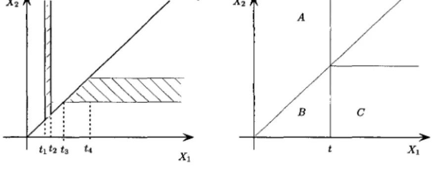
Figure 1.1 shows the (X1,X2) plane and the events whose probabilities

can be estimated from observable data. For example, given times tl

<

t2

we can estimate the probability of the event tl

<

XI 5 t2, XI

<

X2 which

corresponds to the vertical hatched region on the figure, while given times t3

<

t4 we can estimate the probability of the event t3

<

X2

I

t4, XZ

<

XI, which corresponds to the horizontal hatched region on the figure.

Fig. 1.1.

(R)Geometry of events determining the upper and lower bounds.

(L) Events whose probabilities can be estimated by competing risk data;

We are able to estimate the probability of any such region, but we cannot

estimate how the probability is distributed along such a region. Now we can

see why the distribution of X1 is not identifiable; varying the mass within

the horizontal region changes the distribution of XI without changing the distribution of the observable quantities. Considering the “extreme” ways in which that probability mass could be distributed leads to upper and lower bounds on the marginal distribution function of XI. The Peterson boundsg are pointwise upper and lower bounds on the value of the marginal distribu-

tion function. They say that for any t 2 0 we have Gl(t) 5 Fl(t) 5 F y ( t ) .

A functional bound was found by Crowder’O who showed that the dis-

tance between the distribution function F1 and the Peterson lower bound,

F1 ( t ) - GI ( t ) is nondecreasing.

A simple proof of these bounds is possible through considering the ge-

ometry of the events in the (XI, Xz)-plane. Figure l.l(R) shows, for a given

t, three events marked A , B and C. The probability of event A is the lower

bound probability in the Peterson bound, Gl(t). This is clearly less than or equal to the probability of event A U B , which is just Fl

( t ) .

This in turn

is less than or equal to the probability of event A

u

B

u

C, which is just

This shows that the lower and upper Peterson bounds hold. To get the functional lower bound of Crowder just note that the difference Fl(t)-Gl(t)

is the probability of the event {XI

5

t,X2

<

XI}, that is, the region

marked B on the figure. Clearly as t increases, we get an increasing se-

quence of events whose probabilities must therefore also be nondecreas- ing. This demonstrates the functional bound. Both Peterson and Crowder make constructions to show when there is a joint distribution satisfying the

bounds. A result in Bedford and Meilijsonll however improved these results

slightly while giving a very simple geometric construction, which we now

consider.

1.3. Characterization of Possible Marginals

The characterization tells us exactly which marginal distributions are pos- sible for given subdistribution functions. To simplify things in this pre- sentation we assume that we are only going to deal with continuous (sub)distributions and the reader is referred to Bedford and Meilijsonll for the details of the general case of more than 2 variables, which may have atoms and could have ties.

The key idea here is that of a co-monotone representation. We have already seen that the Crowder functional bound writes the distribution

function as a sum of two monotone functions: the subdistribution function

and the nondecreasing “gap.” More generally we define a co-monotone rep-

resentation of a continuous real-valued function f as a pair of monotone

nondecreasing continuous functions f1 and f 2 such that f = f1

+

f2.

The characterization result will show when we can find a pair of ran-

dom variables compatible with the observable subdistribution functions. It

is therefore necessary to define abstractly what a pair of subdistribution

functions is without reference to a pair of random variables. We define a

pair of functions GI, G2 to be a lifetime subdistribution pair if

(1) Gi : [0, m) -+

IR,

i = 1 , 2 .

(2) They are nondecreasing continuous real-valued functions with Gl(0) =

(3) limt-.+oo Gl(t) = pl and limt+oo G2(t) = p2 with pl

+

p2 = 1.

Gz(0) = 0.

Suppose we are given such a pair of functions. (As stated above, the sub-

distribution functions can be estimated from competing risk data.) Consider

the unit strip [0, co) x [0,1] and subdivide it into two strips of heights pl and

the functions G l ( t ) and Gz(t), respectively. In the same strips we choose, arbitrarily, two nondecreasing right continuous functions whose graphs in- crease from the bottom to the top of the strip, while lying under the graphs of the functions we have already drawn. For reasons that will become clear

we call these new functions F2 - G2 and Fl

-

GI, respectively. See Fig. 1.3.

The notion of “lying under” will be made clear in the statement of the

theorem below.

Fig. 1.2. Co-monotone construction - 1

Theorem 1.1: l 1 (i) Let X1 and X2 be lifetime random variables. Then,

using the notation established above,

(1) Fi = Gi

+

(Fi - G , ) is a nonnegative co-monotone representation of a

(2) Fi(t)

5

G l ( t )

+

G z ( t ) for all t , and the Lebesgue measure of the range

(3)(a) Fi(0) = 0 and

Fi(cm)

= 1, for i = 1 , 2 .

nondecreasing continuous function, for i = 1 , 2 .

set

{(Fi

- G i ) ( t ) l F i ( t ) = G l ( t )

+

G 2 ( t ) } is zero, for i = 1 , 2 .

(b) G i ( w )

+

G2(00) = 1 .

(ii) If nondecreasing right continuous functions F1, Fp, GI, and G2 satisfy

the conditions (1)-(3) of (i) then there is a pair of random variables ( X I , Xp)

for which Fi and Gi are the distribution and subdistribution functions

respectively (i = 1,2).

The construction of the random variables ( X I

,

X2) can be done quite simply

and is shown in Fig. 1.3. Draw a uniform random variable U . If it is in the

lower strip (that is, U

<

p1) then we can invert U through the functions

drawn in the lower strip. Define X I = G , ’ ( U ) and Xp = (F2 - G 2 ) - l ( V ) .

The ordering of these two functions implies that X1

5

Xp, and furthermore

that X1 = X2 with probability 0. If U is in the upper strip then a similar

construction applies with the roles of X1 and X , reversed. See Fig. 1.3. This geometrical construction shows that the conditions of the theorem are sufficient for the existence of competing risk variables. Condition 1 is necessary as it is Crowders functional bound. Condition 3 is an obvious

necessary condition. The first part of Condition 2 is the Peterson upper

bound, while the second part is a rather subtle “light t o u c h condition whose proof is fairly technical and for which we refer the reader to Bedford and Meilijson.

1.4. Kolmogorov-Smirnov Test

The complete characterization described above was used to produce a sta- tistical test based on the Kolmogorov-Smirnov statistic in which a hypoth- esized marginal distribution can be tested against available data. The func- tional bound tells us that, given a dataset, the difference between the em- pirical subdistribution and the unobserved empirical marginal distribution

function should be nondecreasing. A little thought shows that the distances

can be computed at the “jumps” of these functions, which of course occur at the times recorded in the dataset. Recall that the Kolmogorov-Smirnov test takes a hypothesized distribution and uses the asymptotic relation that the

functional difference between true population distribution and empirical distribution converges, when suitably normalized, to a Brownian bridge.

Extremes of the Brownian bridge can then be used to establish classical

confidence intervals. Although in our competing risk situation we cannot estimate the maximal difference between empirical distribution function

and hypothesized distribution function (as we are not able to observe the

empirical distribution function), the functional bound can be used to give

lower bound estimates on that maximal difference, thus enabling a conser-

vative Kolmogorov-Smirnov test to be developed.

A

dynamic programming

algorithm can be used to determine the maximum difference. Theoretical details of the test are in Bedford and Meilijson" with more implementation details about the dynamic programming and application examples given in Bedford and Meilijson.12

1.5. Conservatism of Independence

As we noted at the beginning, commercial reliability databases make use of competing risk models in interpreting and presenting data. Common as-

sumptions are that underlying times to failure from different failure modes

are exponential and that the censoring is independent. Clearly, assumptions need to be made, but one can ask whether or not these assumptions are going to bias the numerical results in any consistent way. It turns out that the functional bounds can be used to show that the assumption of inde-

pendence tends to give an optimistic assessment of the marginal of XI. It

was shown in Bedford and Meilijson13 that any other dependence structure would have given a higher estimate of the failure rate; the "independent" failure rate is the lower endpoint of the interval of constant failure rates compatible with the competing risk data. This result, which is generalized to a wider class of parametric families (those ordered by monotone likeli- hood ratio), is essentially based on a constraint implied by differentiating the functional bound at the origin. Consider the following simple example from Bedford and Mei1ij~on.l~

Suppose that the lifetime Y of a machine is exponentially distributed,

there are two failure modes with failure times Xi, X2, and its cause of

failure I = 1 , 2 is independent of Y . Suppose also that the failure rate of

Y is 0 and let P ( I = 1) = pl. The unique independent model (X1,Xz)

for this observed data joint distribution makes Xi and X2 exponentially

distributed with respective failure rates plB and (1 - pl)0.

distribution, but we are not sure about possible dependence. What is

then the range of possible values of its failure rate A? Since the sub-

distribution function of X1 is G l ( t ) = (1

-

e - e t ) p l and X must satisfy F { ( t ) = (1

-

edXt)’ 2 G i ( t ) for all t

>

0, we have that p l 8

5

X

5

8.

The upper Peterson bound tells us that A

5

8. However, the “light touch”

condition discussed above shows that equality is not possible thus giving a

range of feasible X values as

5 x

e

. (1)

This shows that the lowest, most optimistic, failure rate compatible with the general competing risk bounds is that obtained from the independence assumption.

1.6. The Bias of Independence

As a further illustration of the potential bias created by assumption of

independence when it is not clearly appropriate we consider an example

from reliability prediction discussed in Bedford and C00ke.l~ This gives the

theoretical background to work carried out for a European Space Agency

project. Four satellites were due to be launched to carry out a scientific

project, which required the functioning of all satellites throughout the mis-

sion period of 2 years post launch. A preliminary assessment of the satellite

system reliability using a standard model (independent exponentially dis-

tributed lifetimes of subsystems) indicated a rather low probability of mis-

sion success. The study included discussions with mission engineers about the mechanisms of possible mission failure which suggested that, in contrast to the assumptions made in the standard reliability modeling, mission risk was highly associated to events such as vibration damage during launch and satellite rocket firing, and to thermal shocks caused by moving in and

out of eclipses. A new model was built in which the total individual satellite

failure probability over the mission profile was kept at that predicted in the original reliability model. Now, however, a mission phasedependent fail- ure rate was used to capture the engineering judgement associating higher

failure rates to the abovementioned mission phases, and a minimally infor-

mative copula was used to couple failure rates to take account of residual couplings not captured by the main effects.

The effect of positive correlation between satellite lifetimes is to improve system lifetime. This may seem counter intuitiveespecially to those with an engineering risk background used to thinking of common cause effects as being a “bad thing.” However, it is intuitively easy to understand. For

if we sample 4 positively correlated lifetime variables all with marginal

distribution F then the realizations will tend to be more tightly bunched

as compared t o the 4 independent realizations from the same marginal

distribution F . Hence the series system lifetime, which is the minimum of

the satellite lifetimes, will tend to be larger when the lifetimes are more

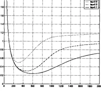
highly correlated. This is illustrated in Fig. 1.4, taken from Bedford and

Cooke,14 which is based on simulation results.

---

Fig. 1.4. Cluster system survival probability depending on correlation.

1.7. Maintenance as a Censoring Mechanism

One very interesting and practical area of application of competing risk ideas is in understanding the impact of maintenance on failure data. There is a lot of anecdotal evidence to suggest that there can be major differences in performance between different plant (for example nuclear plant) that are

not caused by differences in design or different usage patterns, and that

are therefore likely to be related to different maintenance practices and/or policies.

Theoretical models for maintenance optimization require us to know the

lifetime distribution of the components in question. Therefore it is major

our knowledge of that distribution due t o current maintenance (or other) practices that censor the lifetime variable of interest.

1.7.1. Dependent copula model

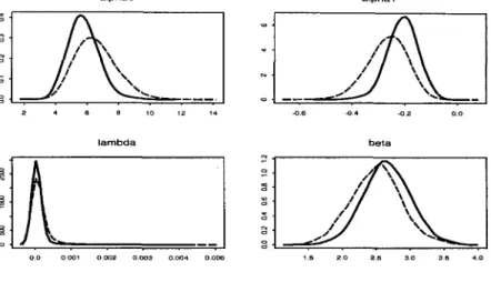
The sensitivity of predicted lifetime t o the assumptions made about de-

pendency between P M and failure time was investigated in Bunea and

Bedford15 using a family of dependent copulae. This is based on the results in Zheng and Klein" where a generalization of the Kaplan-Meier estimator is defined that gives a consistent estimator based on an assumption about the underlying copula of ( X I , X z ) .

To illustrate this in an optimization context, the interpretation given was that of choosing an age-replacement maintenance policy. Existing data,

corresponding t o failure and/or unscheduled P M events, is taken as input.

In order to apply the age replacement maintenance model we need the lifetime distribution of the equipment. Hence it is necessary t o "remove"

the effect of the unscheduled P M from the lifetime data.

The objective was t o show what the costs of assuming the wrong model would be, if one was trying to optimize an age replacement policy. The conclusion of this paper is that the costs of applying the wrong model can indeed be very substantial. The costs arise because the age replacement in- terval is incorrectly set for the actual lifetime distribution when the lifetime distribution has been incorrectly estimated using false assumptions about

the form of censoring. See Fig. 1.5, taken from Bunea and Bedford.15

1.7.2. R a n d o m clipping

This is not really a competing risk model, but is sufficiently close t o be included here. The idea, due t o Cooke, is that the component life time is exponential, and that the equipment emits a warning at some time be- fore the end of life. That warning period is independent of the lifetime of the equipment, although we only see those warnings that occur while the equipment is in use. The observable data here is the time at which the warn- ing occurs. An application of the memoryless property of the exponential distribution shows that the observable data (the warning times) has the

same distribution as the underlying failure time. Hence we can estimate

the MTBF just by the mean of the the warning times data. This model, and the following one, is discussed further in Bedford and C00ke.l~

Fig. 1.5. Optimizing to the wrong model: effect of assuming different correlations.

1.7.3. Random signs

This model" uses the idea that the time at which P M might occur is related

t o the time of failure. The PM (censoring time) X2 is equal t o the failure

time X1 plus an a random quantity

[, X2

= X I -

6.

Now, while [ might not

be statistically independent of X I , its sign is. In other words PM is trying to

be effective and t o occur round about the time of the failure, but might miss the failure and occur too late. The chance of failure or P M is independent of

the time a t which the failure would occur. This is quite a plausible model,

but is not always compatible with the data. Indeed, Cooke has shown that the model is consistent with the distribution of observable data if and only

if the normalized subsurvivor functions are ordered. In other words, this

model can be applied if and only if the normalized subsurvivor function for X I always lies above that for X2.

1.7.4. LBL model

This model, proposed in Langseth and L i n d q ~ i s t , ' ~ develops a variant of the random signs model in which the likelihood of an early (that is, before failure) intervention by the maintainer is proportional t o the unconditional

failure intensity for the component. Maintenance is possibly imperfect in this model. The model is identifiable.

1.7.5. M i z e d exponential model

A new model capturing a class of competing risk data not previously COV-

ered by the above was presented in Bunea et a1.” The underlying model is

that X I is drawn from a mixture of two exponential distributions, while X 2

is also exponential and independent of X I . This is therefore a special case

of the independent competing risks model, but in a very specific paramet- ric setting. Important features of this model that differ from the previous models are: (1) The normalized subdistribution functions are mixtures of

exponential distribution functions, (2) The function @ ( t ) increases contin-

uously as a function o f t . This model was developed for an application to OREDA data in which these phenomena were observed.

1.7.6. D e l a y time model

The Delay time modelz1 is well known within the maintenance community.

Here the two times X1 and X2 are expressed in terms of a warning variable

and supplementary times, X1 = W + X 1 ’ , X z = W + X z ’ , where W, Xl’,XZ’

are mutually independent life variables. As above we observe the minimum

of X 1 and X2.

In the case that these variables are all exponential it can be shown (see Hokstadt and Jensen”) that (a) The normalized subdistribution functions

are equal and are exponential distribution functions, (b) The function @ ( t )

is constant as a function o f t .

1.8. Loosening the Renewal Assumption

The main focus of the paper is on competing risks, and this implies that when we consider a reliability setting we are assuming that the data can be interpreted as though generated by a renewal process. In practice this is not always a good assumption. In general, the higher the risk is that is potentially caused by failure of the equipment and the lower the cost of repair, the more likely it is that maintenance crew will try to get the system back to a “good as new state.”

As discussed in the introduction, the competing risk identifiability ques-

tion is part of the general issue of model identifiability. It is natural there-

system it is quite natural to think about three types of maintenance pro-

grams. The first is “good as new,” that is, when one component fails, all

components are restored to as good as new, thus enabling us to make an

assumption of a renewal process. The second is partial renewal: only the component that fails is restored to as good as new. The fact that the other component(s) are not new may lead t o extra stress being placed on all com-

ponents. The third possibility is “as bad as where a minimal repair is

applied to the failed component that restores it to the functioning state but

leaves the failure intensity for the whole system in the same state as just

before the failure. This situation is discussed by Bedford and L i n d q v i ~ where it is assumed that each component has a failure intensity depending on the components own lifetime plus another term that depends on the age

of each component.

In this context, identifiability means that we can estimate the failure intensities of the components using data from a single socket. This means that we start off with a single unit and replace the components according to the maintenance policy that was determined, recording failure times as we go.

As stated above, the “good as new” policy essentially means that we

are in the classical competing risk situation. Our model class is sufficiently general that it is not identifiable. The least “intensive” maintenance pol- icy, the “bad as old” policy is also not identifiable (indeed, from a single socket data we never revisit any times, so cannot possibly make estimates of failure probabilities). The partial repair policy, however, is rather differ- ent. Here, at least under some quite reasonable technical conditions, we are able to identify the model. The reason for this is enlightening. We can con- sider the vector valued stochastic process, which tells us the current ages of the components at each time point. This process has no renewal properties whatsoever in the minimal repair case. In the full and partial repair cases however it can be considered as a continuous time continuous state Markov process. However, in the full repair case there is no mixing, whereas the partial repair case (under suitable technical, but weak, conditions) the pro- cess is ergodic. This ergodicity implies that a single sample path will (with

probability 1) visit the whole sample space, thus enabling us to estimate

the complete intensity functions.

1.9. Conclusion

(Dependent) competing risk models are increasingly being developed to s u p port the analysis of reliability data. Because of the competing risk problem we cannot identify the joint distribution or marginal distributions without making nontestable assumptions. The validation of such models on a sta- tistical basis is therefore impossible, and validation must therefore be of a “softer” nature, relying on assessment of the engineering and organizational

context. This is particularly so in the area of maintenance policy. Clearly,

there is a whole area of modeling that can be developed.

Acknowledgments

I would like to thank my various collaborators over the last few years in-

cluding Isaco Meilijson (Tel Aviv University)

,

Bo Lindqvist (NTNU Trond-

heim), Cornel Bunea (George Washington University), Hans van der Weide (TU Delft), Helge Langseth (NTNU Trondheim), Sangita Karia Kulathinal

(National Public Health Institute, Helsinki), Isha Dewan (IS1 New Delhi),

Jayant Deshpande (Pune University)

, Catalina Mesina

(Free University,

Amsterdam) and especially Roger Cooke (TU Delft) who introduced me to the area.

References

1. R. Cooke and T. Bedford, Reliability Databases in Perspective, IEEE Trans- actions on Reliability 51, 294-310 (2002).

2. M. Crowder, Classical competing risks, Chapman and Hall/CRC (2001).

3. J. V. Deshpande, Some recent advances in the theory of competing risks, Presidential Address, Section of Statistics, Indian Science Congress 84th Ses- sion (1997).

4. A. Tsiatis, A nonidentifiablility aspect in the problem of competing risks, Proceedings of National Academy of Science, USA 72, 20-22 (1975). 5. E. L. Kaplan and P. Meier, On the identifiability crisis in competing risks

analysis, Journal of American Statistical Association 53, 457-481 (1958). 6. A. NBdas, On estimating the distribution of a random vector when only the

smallest coordinate is observable, Technometrics 12, 923-924 (1970). 7. D. R. Miller, A note on independence of multivariate lifetimes in competing

risk models, A n n . Statist. 5, 576-579 (1976).

8. J. A. M. Van der Weide and T. Bedford, Competing risks and eternal life,

Safety and Reliability (Proceedings of ESREL’98), S. Lydersen, G.K. Hansen,

H.A. Sandtorv (eds), Vol. 2, 1359-1364, Balkema, Rotterdam (1998).

9. A. Peterson, Bounds for a joint distribution function with fixed subdistribu- tion functions: Application to competing risks, Proc. Nat. Acad. Sci. USA 73,

10. M. Crowder, On the identifiability crisis in competing risks analysis, Scand. J . Statist. 18, 223-233 (1991).

11. T. Bedford and I. Meilijson, A characterization of marginal distributions of (possibly dependent) lifetime variables which right censor each other, Annals of Statistics 25, 1622-1645 (1997).

12. T. Bedford and I. Meilijson, A new approach to censored lifetime variables, Reliability Engineering and System Safety 51, 181-187 (1996).

13. T. Bedford and I. Meilijson, The marginal distributions of lifetime variables which right censor each other, in H. Koul and J. Deshpande (Eds.), I M S

Lecture Notes Monograph Series 27 (1995).

14. T. Bedford and R. M. Cooke, Reliability Methods as management tools: dependence modelling and partial mission success, Reliability Engineering and System Safety 58, 173-180 (1997).

15. C. Bunea and T. Bedford, The effect of model uncertainty on maintenance optimization, I E E E Transactions in Reliability 51, 486-493 (2002).

16. M. Zheng and J. P. Klein, Estimates of marginal survival for dependent competing risks based on an assumed copula, Biometrika 82, 127-138 (1995). 17. T. Bedford and R. Cooke, Probabilistic Risk Analysis: Foundations and

Methods, Cambridge University Press (2001).

18. R. Cooke, The total time on test statistic and age-dependent censoring, Stat. and Prob. Let. 18 (1993).

19. H. Langseth and B. Lindqvist, A maintenance model for components exposed to several failure mechanisms and imperfect repair, in B. L. K. Doksum (Ed.),

Mathematical and Statistical Methods in Reliability, pp. 415-430. World Sci- entific Publishing (2003).

20. C. Bunea, R. Cooke, and B. Lindqvist, Competing risk perspective over re- liability databases, in H. Langseth and B. Lindqvist (Eds.), Proceedings of Mathematical Methods in Reliability, NTNU Press (2002).

21. A. Christer, Stochastic Models in Reliability and Maintenance, Chapter A re-

view of delay time analysis for modelling plant maintenance, Springer (2002). 22. P. Hokstadt and U. Jensen, “Predicting the failure rate for components that

go through a degradation state,” Safety and Reliability, Lydersen, Hansen and Sandtorv(eds) Balkema, Rotterdam, pp. 389-396, (1998).

23. T. Bedford and B. H. Lindqvist, The Identifiability Problem for Repairable Systems Subject to Competing Risks, Advances in Applied Probability 36,

GAME-THEORETIC AND RELIABILITY METHODS IN

COUNTER-TERRORISM AND SECURITY

VICKI BIER

Center f o r Human Performance and Risk Analysis University of Wisconsin-Madison

Madison, Wisconsin, USA E-mail: bier@engr.wisc.edu

The routine application of reliability and risk analysis by itself is not adequate in the security domain. Protecting against intentional attacks is fundamentally different from protecting against accidents or acts of nature. In particular, an intelligent and adaptable adversary may adopt

a different offensive strategy to circumvent or disable protective secu- rity measures. Game theory provides a way of taking this into account. Thus, security and counter-terrorism can benefit from a combination of reliability analysis and game theory. This paper discusses the use of risk and reliability analysis and game theory for defending complex systems against attacks by knowledgeable and adaptable adversaries. The results of such work yield insights into the nature of optimal defensive invest- ments in networked systems to obtain the best tradeoff between the cost of the investments and the security of the resulting systems.

2.1. Introduction

After t h e September 11, 2001, terrorist attacks on the World Trade Cen- ter and the Pentagon, and the subsequent anthrax attacks in t h e United States, there has been an increased interest in methods for use in security

and counter-terrorism. However, the development of such methods poses two challenges t o the application of conventional statistical methods-the relative scarcity of empirical data on severe terrorist attacks and t h e inten- tional nature of such attacks.

In dealing with extreme events, for which empirical data is likely t o

be sparse, classical statistical methods have been of relatively little use.'

17

Instead, methods such as reliability analysis are used to break complex sys-

tems down into their individual components (such as pumps and valves)

for which larger amounts of empirical failure-rate data may be available. Risk analysis2i3 builds on the techniques of reliability analysis, adding consequence-analysis models to allow for estimation of health and safety impacts. Quantification of risk-analysis models generally relies on some combination of expert judgment4 and Bayesian statistics to estimate the pa-

rameters of interest in the face of sparse data.5 Zimmerman and Bier‘ argue

that “Risk assessment in its current form (as a systems-oriented method that is flexible enough to handle a variety of alternative conditions) is a vital tool for dealing with extreme events.”

However, the routine application of reliability and risk analysis by itself is not adequate in the security domain. Protecting against intentional at-

tacks is fundamentally different from protecting against accidents or acts of

nature (which have been the more usual focus of engineering risk analysis). In particular, an intelligent and adaptable adversary may adopt a differ-

ent offensive strategy to circumvent or disable protective security measures.

Game theory7 provides a way of taking this into account analytically. Thus,

security analysis can benefit from a combination of techniques that have not usually been used in tandem. This paper discusses approaches for us- ing risk and reliability analysis and game theory to defend complex systems against intentional attacks.

2.2. Applications of Reliability Analysis to Security

Early applications of engineering risk analysis to counter-terrorism and se-

curity include Martz and Johnson’ and

COX.^

More recently (following

September ll), numerous risk analysts have proposed its use for home- land security.10-13 Because security threats can span such a wide range, the emphasis has been mainly on risk-based decision making (i.e., using

the results of risk analyses to target security investments at the most likely

and most severe threats). Much of this work has been directed specifically

towards threats against critical infrastructure14- l9 Levitin and colleagues

have by now amassed a large body of work applying reliability analysis to security problems.20-22

Risk and reliability analysis have a great deal to contribute to ensuring the security of complex engineered systems. However, unlike in applications of risk analysis to problems such as the risk of nuclear power accidents, the relationship of recommended risk-reduction actions to the dominant risks