Construction and characterization of a universally tunable modulator

Construction and Characterization of a

Universally Tunable Modulator

by

Sarah Ackley

Submitted to the Department of Physics

in partial fulfillment of the requirements for the degree of

Bachelor of Science in Physics

at the

MASSACHUSETTS INSTITUTE OF TECHNOLOGY

May 2008

©

Massachusetts Institute of Technology 2008. All rights reserved.

'---,

Author ...

Department of Physi

May 9, 2008

Certified by ...

Nergis Mavalvala

Associate Professor

Thesis Supervisor

Accepted by

MASSACHUSETTS INST[TUTE OF TECHNOLOGY

JUN

13

2008

LIBRARIES

David Pritchard

Chairman, Professor

Construction and Characterization of a Universally Tunable

Modulator

by

Sarah Ackley

Submitted to the Department of Physics on May 9, 2008, in partial fulfillment of the

requirements for the degree of Bachelor of Science in Physics

Abstract

Arbitrary admixtures of amplitude and phase modulated light can be used to gener-ate linear, null-crossing error signals for locking Fabry-Perot cavities that are detuned from resonance by arbitrary amounts. Unfortunately, no commercially available de-vice is capable of producing the desired arbitrary combinations of amplitude and phase modulation. This work pertains to construction and characterization of a Uni-versally Tunable Modulator (UTM), capable of producing just such combinations. The UTM was prototyped by modifying a New Focus 4104 amplitude modulator. With the application of feedback control of fabry-perot cavities in mind, the UTM was characterized using a test cavity to measure error signals. The resulting error signals were then fit to the calculated error signals to give the fractions of amplitude and phase modulation. It was shown that it is possible to produce nearly pure am-plitude and phase modulation, as well as intermediate modulation states, using the UTM. The resulting error signals also indicate the UTM's suitability for both on- and off-resonance locking of Fabry-Perot cavities.

Thesis Supervisor: Nergis Mavalvala Title: Associate Professor

Acknowledgments

I would like to thank Prof. Mavalvala for the opportunity to work on LIGO, and on this thesis project. Prof. Mavalvala was extremely helpful in answering my questions, assisting me in lab, and editing this thesis. I also appreciate all the advice Prof. Mavalvala has given me outside the context of this experiment.

The graduate students in Prof. Mavalvala's group were also extremely helpful; their assistance was vital to the completion of this project. I am particularly grateful Chris Wipf for his ability to explain science clearly and well and his patience in doing so, as well as his extensive assistance in lab. One night he spent 8 hours nonstop helping me get my experiment working again. Thomas Corbitt's help was invaluable; on numerous occasions he assisted me in lab and answered my questions. He also put substantial effort into helping to plan this experiment. In particular, I should credit him with the alternative UTM characterization method described in this thesis. I would also like to thank Tim Bodiya and Nicolas Smith for both their help and company while working in lab. Tim, in particular, spent several hours straight one night helping me get my experiment working, as well as helping me on numerous other occasions.

I would also like to thank Chris and Tim for cleaning up before floor waxing and Shaunalynn Duffy for proof reading the final version of my thesis.

Contents

1 Introduction 15

1.1 Applications to LIGO . . . . 16

1.2 O verview . . . . 17

2 Fabry-Perot Cavities 19 2.1 The Flat-Mirror Cavity ... 20

2.2 Spherical-Mirror Cavities ... 21

2.3 Mode-Degenerate Interferometer . . . . 22

3 Modulation Using Electrooptic Crystals 23 3.1 Amplitude and Phase Modulation . . . . 23

3.2 The Electrooptic Effect ... 23

3.3 Amplitude and Phase Modulation . . . . 25

3.3.1 Amplitude Modulation with KDP . . . . 27

3.3.2 Phase Modulation with KDP . . . . 27

3.3.3 Amplitude and Phase Modulation with Lithium Niobate . . . 28

4 Pound-Drevor-Hall Locking 29 4.1 A Calculation of an Amplitude-Modulation Error Signal . . . . 30

5 Experimental Design 35 5.1 UTM Design and Construction ... 35

6 Characterization of the New Focus Amplitude Modulator and UTM 41 7 Data Analysis

7.1 Results.... . . .... ... . 45 7.2 Discussion and Conclusions ... ... 50 A UTM Alignment Procedure

List of Figures

2-1 A Fabry-Perot cavity. The curved red lines indicate the shape of a stable cavity mode; that is, a mode which reproduces itself which each reflection . . . 19 2-2 Transmitted intensity, or power, as a function of frequency detuning,

v - vo, for a Fabry-Perot cavity. ... 21

3-1 A modulation signal can be encoded in a carrier using amplitude or

phase modulation. ... 24

3-2 Left: A KDP crystal without an applied voltage. Light enters on the front face and passes through the crystal in the z direction. Right: A KDP crystal with an applied voltage V, showing how the [X, Y, Z] coordinate system transforms into the [Ix, y, z] coordinate system. Ap-plying a voltage allows for modulation . . . . . . 27

4-1 Error signal as a function of detuning from resonance for PDH locking using phase-modulated light (a), amplitude-modulated light (b), and equal amounts of amplitude- and phase-modulated light (c). The cav-ity transmission as a function of frequency is shown in (d). Note that

the error signal is approximately linear near the zero-crossings. . . . 31

4-2 The simplified layout for locking a cavity to a laser with amplitude modulated light. The solid, red lines indicate the optical path, whereas the dashed lines indicate the signal paths . . . . 32

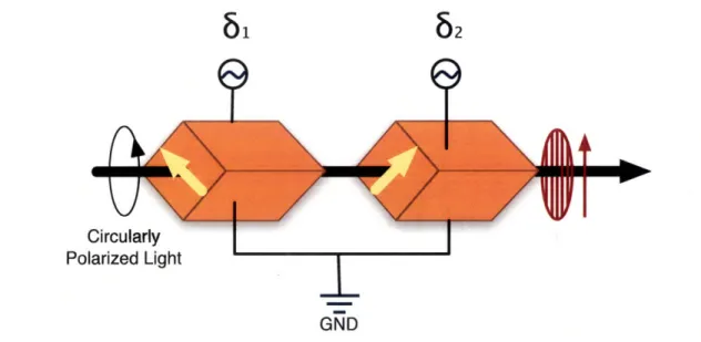
5-1 Schematic of the UTM. The two LN crystals are placed in series, mounted with modulation axes, indicated by yellow arrows, at 900

with respect to one another. The thick black arrow shows the beam path. The input light is circularly polarized and a polarizer is placed at the output of the crystals; this allows for access to all modulation

states by separately varying the voltage inputs, 31 and 62. . . . . . . 36

5-2 Left: New Focus amplitude modulator prior to modification. Right: New Focus amplitude modulator post-modification, or UTM. The op-tical axis is along the length of the two crystals . . . . . 36 5-3 Photograph of the characterization setup. The red arrows indicate the

beam path. . . . 38 5-4 Schematic of the characterization setup. UTM: universally tunable

modulator; PBS: polarizing beam splitter; A/4: quarter waveplate; A/2: half waveplate; PD: photodetector; RF: high frequency output; LO: local oscillator. The red arrows indicate the beam path . . . . . 38

6-1 Setup for characterization of the New Focus amplitude modulator. . 41

6-2 The amount of amplitude modulation is maximized with incident cir-cularly polarized light or with vertically polarized light incident and a DC (direct current) voltage such that the transmission percentage is h alf. . . . 42 6-3 Modulation signal with circularly polarized light (blue) and linearly

vertically polarized light (red). The New Focus amplitude modulator (before modification) was driven with a 25 MHz signal in both cases. The blue curve corresponds to the operating point with half of the input intensity exiting the modulator. The red curve corresponds to a maximum of vertically polarized light out of the modulator. Thus, both the 25 MHz modulation signal and 50 MHz sideband are present. 43

6-4 Plot of AC voltage (peak-to-peak) over DC voltage out of the amplitude modulator (left) and UTM acting as an amplitude modulator (right) versus the input voltage of the modulation signal (25 MHz). Data points with error bars shown in red are fit to a line shown in blue. . 44

7-1 Nearly amplitude modulation error signal (top) with cavity transmis-sion shown (bottom). Measured signals are shown in black and fits in red . . . . 46 7-2 Nearly phase modulation error signal (top) with cavity transmission

shown (bottom). Measured signals are shown in black and fits in red. 47 7-3 Combination amplitude and phase modulation error signal (top) with

cavity transmission shown (bottom). Measured signals are shown in black and fits in red . ... 48

List of Tables

5.1 Inputs into the UTM's two crystals and resulting modulation states. 39 7.1 Fractions of amplitude and phase modulation for nearly amplitude,

nearly phase, and combination amplitude and phase modulation oper-ating points. Averages with standard deviations are shown . . . . . 50 7.2 Amount error signals are shifted below resonance in units of cavity

Chapter 1

Introduction

Amplitude and phase modulators of light are widely used in modern optics. However, there is no single commercial device that allows for controllable amounts of amplitude and phase modulation with complete variability. If variable amounts of amplitude and phase modulation are needed, the only commercially available option is to use a cumbersome optical setup, such as an amplitude modulator and phase modulator in series or two phase modulators in a Mach-Zehnder configuration. Cusack et al. at Australian National University built a prototype of such a device, called a universally tunable modulator or UTM[1]. For my thesis, I constructed and characterized a UTM, following a construction procedure similar to that of Cusack et al, but a different characterization procedure.

The UTM is constructed by modifying a commercially available amplitude modu-lator; the amplitude modulator is rewired such that its two crystals are controlled by separate inputs, rather than just one input. The phrase universally tunable empha-sizes that the modulator is capable of both amplitude modulation, phase modulation, and combinations thereof with complete control over the relative phases between the two types of modulation.

An anticipated use for the UTM is optical feedback control of a Fabry-Perot cavity to maintain the cavity on-resonance or near resonance. With this anticipated use in mind, Cusack et al.'s characterization procedure was modified; instead of directly measuring the relative amounts of amplitude and phase modulation, a test cavity was

used to measure the feedback signal. By fitting the feedback signal, it is also possible to determine the amounts of amplitude and phase modulation. Additionally, the optical feedback application was directly tested to maintain the resonance condition of the cavity.

1.1

Applications to LIGO

Gravitational waves are predicted by Einstein's General Theory of Relativity. Just as accelerated charges produce photons, the carrier of electromagnetic waves, it is predicted that accelerating masses produce gravitational waves. So far, there is only indirect experimental evidence for their existence; scientists have not yet directly measured gravitational waves[2].

LIGO (Laser Interferometer Gravitational Wave Observatory), the National Sci-ence Foundation's largest funded project, as well as its sister projects in Europe and Japan, endeavor to directly measure gravitational waves. LIGO has two observatories, located in Washington and Louisiana, equipped with 4 km-long, vacuum-enclosed, and seismically-isolated cavities. These cavities are locked to a particular operating point; then, the feedback, or error, signal on these cavities is measured. An incom-ing gravitational wave would change the length of the cavity, causincom-ing a feature in the feedback signal; the feedback signal is thus measured to obtain direct evidence and measurements of gravitational waves[2]. Advanced LIGO, the next generation of LIGO scheduled for 2013, involves cavities that will be operated off-resonance. The UTM is a tool which produces clean linear signals for Fabry-Perot cavities with arbi-trary detuning from resonance[3]. While Advanced LIGO could make use of UTMs to work off-resonance, the UTM I built will be used extensively in Professor Mavalvala's group to study some of the implications of working off-resonance, as well as other future applications to LIGO. To name but a few examples from Prof. Mavalvala's lab, studies on radiation pressure dynamics and pondermotive squeezing, as well as the experiments aimed at finding the quantum mechanical behavior of macroscopic objects all require off-resonance locking of Fabry-Perot Cavities[4][5][6].

1.2

Overview

Chapter 2 gives an overview of the physics behind Fabry-Perot cavities with partic-ular attention given to the confocal cavity used in this experiment. Chapter 3 covers how modulation is achieved with electrooptic crystals, specifically the methods be-hind producing amplitude and phase modulation. Chapter 4 discusses how locking is achieved using the Pound-Drevor-Hall technique; this chapter explicitly derives how amplitude modulated light allows for off-resonace locking. Chapter 5 gives a descrip-tion of the experimental design, detailing both the construcdescrip-tion of the UTM and its characterization. Chapters 6 and 7 present the results: the characterization of the amplitude modulator, before and after modification, and the measurement of error signals, respectively.

Chapter

2

Fabry-Perot Cavities

Fabry-Perot cavities, or interferometers, used frequently in optical physics, have a variety of applications, from laser construction to analyzing an optical spectrum to frequency stabilization of a laser. In LIGO, for example, cavities are used to detect tiny length changes as a result of gravitational waves. As shown in figure 2-1, a

Fabry-Perot cavity consists of two mirrors, separated by some distance d. Usually, curved mirrors are used because they are far less sensitive to misalignment; the optical mode confined by two flat mirrors is unstable as it has the tendency to "walk-off' the cavity axis[7].

With such a curved-mirror arrangement, it is possible to distinguish two types of laser modes: longitudinal modes differ only in oscillation frequency, whereas

trans-I

d ' "

Figure 2-1: A Fabry-Perot cavity. The curved red lines indicate the shape of a stable cavity mode; that is, a mode which reproduces itself which each reflection.

verse modes differ not only in oscillation frequency, but also in the spatial distribution

of the field in the plane perpendicular to the direction of propagation[7].

2.1

The Flat-Mirror Cavity

We start with the flat-mirror cavity for simplicity. In order for light to build up in such a cavity, or for resonance to occur, the spacing between the mirrors must be an integer number of half wavelengths of the incoming light. Equivalently written,

nc

Vo = (2.1)

2d

where v0 is the frequency of incoming light, n is an integer, c is the speed of light, and d is the mirror separation. The ratio of the transmitted intensity out of the cavity to the input intensity, for highly reflective mirrors with low losses, is given by

I

=-

1

(2.2)

- 1 _{1 +k} + (( _(1-R)) )2

(V -

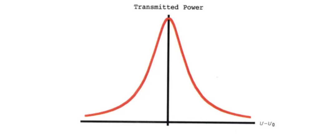
_V 2

where R is the reflectance of each of the mirrors and v the the frequency of the incoming light[7]. Figure 2-2 shows how the transmitted power depends on frequency detuning, v - v0, for a Fabry-Perot cavity.

The electric field coming out of such a cavity can be calculated using what is called a reflection coefficient. The reflected electric field, E,, is given by Einc x F,

where Einc is the field incident on the cavity and F is the reflection coefficient. The reflection coefficient for the confocal cavity used in this experiment near resonance is given by

1 - i(w - wo)/7Y _(2.3)

W) 1 + i(w - wo)/7

where -- = '(1 R, = w/2r = v is the laser frequency, and wo/2-r = vo is the

resonant frequency of the cavity.

We can define two quantities of interest for such cavities: the full-width half maximum (FWHM) and the free-spectral range (FSR). The FWHM is a measure of

Transmitted Power

U-U₀

Figure 2-2: Transmitted intensity, or power, as a function of frequency detuning,

v - vo, for a Fabry-Perot cavity.

the width of the cavity's resonance and is given by

A = c(1 - R) (2.4)

2rd

The FSR is defined as the the frequency difference between two transmission fringes and is given by

c

FSR = -(2.5)

2d

2.2

Spherical-Mirror Cavities

Another problem with flat-mirror Fabry-Perot cavities is that diffraction of the laser beam can lead to significant losses in the outgoing laser power. This can be mitigated to a large extent by the use of spherical mirrors: the diffraction loss of a spherical-mirror interferometer is several orders of magnitude lower than that of a flat spherical-mirror interferometer[7]. The difficulty with these spherical-mirror cavities, however, it that the incoming laser beam must be mode-matched to the cavity; that is, the mode, or wave-front of the beam, must be reproduce itself within the cavity[7].

The modes of such a spherical mirror cavity resonate at the following frequencies:

c

1

₎

Vo =

_2d

-

_I

q+ (1 + m + n)arccos(1 - d/R,) (2.6)

where Rc is the radius of curvature of the mirrors, q is an integer indicating the longitudinal mode number, and m and n denote the transverse mode numbers[7].

2.3

Mode-Degenerate Interferometer

A mode-degenerate interferometer, used in this experiment, is a spherical-mirror in-terferometer whose transverse modes have the same frequency. Such as degeneracy occurs when

arccos(1 - d/R,) = 7r/1 (2.7)

where 1 is an integer. The resonance condition for such a cavity can be rewritten as c

v

= [1q +

_21d

1

+

m

+

n]

(2.8)

Note that increasing m+n by 1 and decreasing q by one, does not change the resonant frequency v0. The confocal interferometer, corresponding to I = 2, is used in this

experiment. For such a cavity, the free-spectral range is given by[7]

c

FSR = - (2.9)

Chapter 3

Modulation Using Electrooptic

Crystals

3.1

Amplitude and Phase Modulation

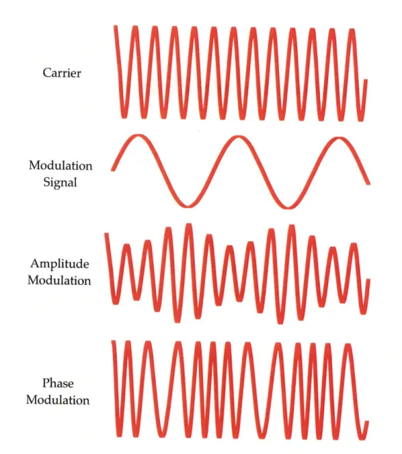
Modulation is the process of encoding information in variations of a waveform's am-plitude or phase. It is possible to modulate both a voltage signal and a light wave; here we are concerned with the latter. Figure 3-1 shows amplitude modulation and phase modulation with a sinusoidal carrier signal, as is used in this experiment. It is the goal of this experiment to create both pure amplitude modulation and phase modulation as shown, as well as combinations of amplitude and phase modulation. The electrooptic effect, described below, is used to achieve the amplitude and phase modulation of light[8].

3.2

The Electrooptic Effect

The electrooptic effect is the change in the refractive index of a material as a result of an applied voltage. For some crystals, such as ADP, KDP, and Lithium Niobate (LN), the refractive index depends linearly on the applied voltage. For other materials, such as liquids and glasses, the dependence of the refractive index on the applied voltage is quadratic. These are known as the linear and quadratic, respectively, electrooptic

Carrier Modulation Signal Amplitude Modulation Phase Modulation

Figure 3-1: A modulation signal can be encoded in a carrier using amplitude or phase modulation.

effects[8]. Here, we only concern ourselves with the linear electrooptic effect, as it is utilized in the construction of modulators.

3.3

Amplitude and Phase Modulation

The first electrooptic light modulator was demonstrated by B. Billings using an ADP crystal. More modern modulators use crystals such as LN, used in this experiment, instead of ADP and KDP, which are sensitive to moisture in the air. Here, however, I will use KDP as an example. Due to the crystal symmetry of KDP, the calculation of the amounts of amplitude and phase modulation are simpler; such a calculation for LN is similar yet slightly more complicated[9]. See appendix B for a calculation involving LN.

An index ellipsoid is an ellipsoid which describes both the orientation of the crys-tal's principle axes as well as the indices of refraction along these axes[9]. For KDP the index ellipsoid in the absence of an electric field is given by

X2 _y2 _ZV

2

+

2

+

2=

1.

(3.1)

where no and ne are the indices of refraction along what are called the ordinary (X and Y) and extraordinary (Z) axes, respectively. For this ellipsoid, the [X, Y, Z] coordinate system is the principle axis coordinate system for the crystal in the absence of an electric field. If a field E = (Es, Ey, E,) is applied, the index ellipsoid becomes

X

2

_y

2

_Z

2

2- + + 2- - + 2r₄1EYZ + 2r41EyXZ + 2r63EzXY = 1 (3.2)

no

no

ne

where r41 and r63 are electrooptic coefficients. Now, suppose that the electric field is applied only along the z-direction. The index ellipsoid becomes

X

2

_y

2

_Z

2

--• - 2 j + 2r 63EzXY = 1. (3.3)

H no ne

coor-dinate system since [X, Y, Z] do not correspond to the principle axes of the ellipsoid. However, this simple substitution reveals the new principle axes:

X =x Y Y = X + Z = z (3.4)

giving the following index ellipsoid

(½+

r

2E

+

-

r

+

63

E

y

2

n

=

1.

(3.5)

n2

no2

n2

This can be rewritten as

x2 y2 2 n + n2 = 1.2 (3.6) where 1 nx ez no - ₂n 3r63Ez (3.7) 1 ny .. no + -n r63Ez (3.8) 2

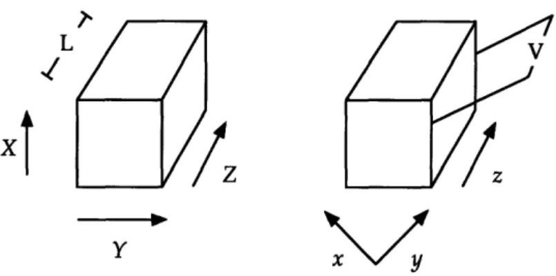
to first order in the applied electric field; such an approximation is valid for the small modulation depths used in this experiemnt. The difference between these two indices of refraction is what allows us to to construct a modulator[8][9]; figure 3-2 shows both the coordinate change with an applied field and how to construct a modulator utilizing the electrooptic effect. Suppose a beam of light, with both x and y polarization components, propagates through the crystal in the z-direction, as shown in figure 3-2. After propagating through the length L of the crystal, the x and y polarization components acquire a phase difference, or retardation, given by

F- (n - nx)wL nr 63EzwL (39)

IF

Y

~

r3Ew

(3.9)

c c

where c is the speed of light. However, Ez = V/L where V is the applied voltage, so

we can rewrite the retardation as[9][8]

nor63wV

IC

d6w V (3.10)

L

X1

Y

Figure 3-2: Left: A KDP crystal without an applied voltage. Light enters on the front face and passes through the crystal in the z direction. Right: A KDP crystal with an applied voltage V, showing how the [X, Y, Z] coordinate system transforms into the [x, y, z] coordinate system. Applying a voltage allows for modulation.

3.3.1

Amplitude Modulation with KDP

To construct an amplitude modulator with a KDP crystal, a vertical (X-direction) po-larizer can be placed before the entrance to the crystal and a horizontal (Y-direction) polarizer can be placed after crystal exit. In this case, the output intensity, Io, takes on the following form

2F

lot = sin2 _{- X Iin (3.11)}

2

where Iin is the input signal. Now, suppose that a sinsusoidal voltage is applied such that the retardation takes the following form

IF = F0 + m coswmt. (3.12)

The transmitted intensity will then be modulated as cos wmt. The maximum mod-ulation will occur when Fo = r/2, which can be achieved either by using a quarter-waveplate[9] or by applying a DC voltage to the crystal.

3.3.2

Phase Modulation with KDP

To construct a phase modulator with a KDP crystal, the incident light is such that it is parallel to either the x- or y-axes, and the polarizers used for amplitude modulation

are removed. Here, the application of a sinusoidal voltage across the crystal simply introduces a sinusoidal phase delay in the phase of the outgoing light[9].

3.3.3

Amplitude and Phase Modulation with Lithium

Nio-bate

Due to their different molecular geometry, modulation with LN is done slightly dif-ferently. The voltage, instead of being applied to the axis parallel to the direction of propagation, is applied to an axis perpendicular to the direction of propagation. In this case then, the applied electric field cannot be written as E = V/L, which means that length fluctuations can affect the depth of amplitude modulation. This is generally solved by using two crystal whose axes are mounted perpendicular to one another such that the length noise induced by one crystal is cancelled out by the length noise in the other.

Chapter 4

Pound-Drevor-Hall Locking

Pound-Drever-Hall (PDH) locking was invented as a technique to stabilize the fre-quency of a laser using a Fabry-Perot cavity[10]. Although PDH locking is primarily used for laser frequency stabilization, it is also used to lock a cavity to a laser-that is, to keep the length of the cavity such that the incident laser frequency will be resonant[10]. PDH locking is used to measure length changes in interferometer cavi-ties, such as those used in the Laser Interferometer Gravitational-wave Observatory

(LIGO) [2].

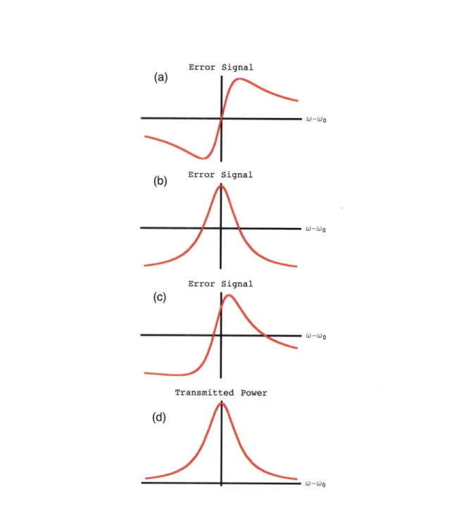
To PDH lock a cavity to a laser, phase-modulated light is incident on a cavity with a partially transmissive input mirror and highly reflective end mirror. The light reflected from the cavity is detected on a fast photodetector and downconverted to DC by mixing with a local oscillator, a modulation signal at the same frequency of the phase-modulation. The resulting signal, or error signal, shown in figure 4-1(a), is

fed back as a force on one of the mirrors to maintain the cavity length corresponding to the laser frequency. Note that for positive and negative deviations in length, the feedback force on the mirror is of opposite signs, thus restoring the cavity to the resonant length[10].

A significant limitation of PDH locking with phase-modulated light is that a lin-ear null-crossing signal is only available at the cavity resonance. Modifying PDH locking by sending in only amplitude-modulated light allows for locking the cavity off-resonance, as shown in figure 4-1(b), but only at one at one of two possible points.

By sending in a mixture of both amplitude and phase-modulated light, it is possible to lock a cavity at any length[1]; figure 4-1(c) shows the feedback signal for equal amounts of amplitude and phase modulation. For other experiments, real-time vari-ability is required, making it necessary to change the amount of amplitude and phase modulation without modifying the optical setup [1].

4.1

A Calculation of an Amplitude-Modulation

Er-ror Signal

Here I derive the error signal for an amplitude-modulated input signal[10], following a procedure similar to that of Black's calculation for phase modulation[10]. A similar calculation can be done for combinations of amplitude and phase modulation.

Figure 4-2 shows the Pound-Drever-Hall setup, using amplitude-modulated light to lock the cavity. The light beam, coming from a laser, is modulated by the amplitude modulator; the source of the modulation signal is also used as the local oscillator for demodulation. In the frequency domain, light that is incident on the cavity is comprised of a carrier that resonates in the cavity and a pair of modulation sidebands that are outside the cavity linewidth.The reflected signal from the cavity, collected on a photodetector, is mixed with the local oscillator signal, resulting in an error signal. The servo controller then amplifies the error signal, which is fed back to the mirror actuator to maintain the cavity at a particular point near resonance as shown in 4-1. We start out with a carrier wave c(t) = Aeiwct. We wish to modulate c(t) with a signal m(t) = sinwmt. We only modulate c(t) by a small percentage which we will denote by 2B/A. We can now write the electric field, Einc, incident on the Fabry-Perot Cavity:

Einc = (A - 2B sin wmt)ei"wct

= Aeiwct

+

iB(ei•wmt - e-iwmt)eiwct

Error Signal Error Signal Error Signal (c) W-WO W WO 60-wO₀ Transmitted Power (d) W-W0

Figure 4-1: Error signal as a function of detuning from resonance for PDH locking using phase-modulated light (a), amplitude-modulated light (b), and equal amounts of amplitude- and phase-modulated light (c). The cavity transmission as a function of frequency is shown in (d). Note that the error signal is approximately linear near the zero-crossings.

Amplitude

\ctuator

- ..- -~ -I

Signal _Transmissive Iarlanuy _Reflectiverigyniy

Photodetector

---

-Local Oscillator Mixer Servo Amp

Figure 4-2: The simplified layout for locking a cavity to a laser with amplitude modulated light. The solid, red lines indicate the optical path, whereas the dashed lines indicate the signal paths.

The reflected field is given by

Erej = AF(wc)ei•Wct _{+BF(wc+Wm)ei[(w}c+_wm)t±/+ 2_{] - BF(w - wm)ei[(w}, -_wm)t+_{7/2] (4.1)}

where F(w) is the reflection coefficient of the cavity. The reflection coefficient for the confocal cavity used in this experiment near resonance is given by

1 - i(w -wo)/Y (4.2)

FkW) = _{r~)=1 + i(w -}± -w~y(4.2)_{0) /7}

where'= cd i = -, and w/27r = v, the laser frequency. The reflected power Pref is therefore given by

Pref = Eref E*~ef

A2

_IF(wc)

1 _{+ B}2_{[ F(w, + Wm)I + IF(w, -W) 2]}

+AB[F(wLc)F*(w, + wm)e-i(wmt+ /2) + F*(we)F(w, + wm)ei(wmt+±/ 2)

-F(wC)F*(w

-

wm)ei(wmt~/2)

-

F*(wc)F(W

-

wm)e-i(wmt-/2)]

-B 2[F(w, + wm)F*(wc - wm)e 2wmt + F*(wC + Wm)F(wc - wm)e-2wmt

A

2

_IF(wc)I

2

₊

_B2[IF(wc

₊

_wm)1

2

_{+ IF(wr}

_{- Wm)1}2]

+iAB[-F(wUc)F*(wU + wm)e -iwmt + F*(wUc)F(wU + wm)eiwmt

+F(wc)F*(wc - wm)eim' t - F*(wc)F(wc - wm)e - iwmt]

-B 2[F(w, + wm)F*(wc - wrm)e2wt + F*(wc + wm)F(wc - Um)e- 2wmt].

To simplify, we can write x, = F(wc)F*(w + wmn) and x2 = F(w)F* (wc - wn). Thus,

the reflected power can be written as:

Pref = constant terms + 2 _{•m terms}

+AB [-ixi(coswmt - isin wmt) + ix*(cos wmt + isinwmt)

+ix2(cos wmt + i sin wmt) - ix* (cos wmt - i sin •mt)]

constant terms + 2wm terms

+2AB[9(xi

- x2)cosWmt- O(x 1 +

x2

)

Sin

•t].I

The mixer picks out terms that oscillate as wmn. The error signal, therefore, is given by either

e= 2ABa(x1 - x2) = 2ABQ[F(wc)F*(wC + wm) - F(wc)F*(wU - wm)] (4.3) or

e = -2ABR(xl + x2) = 2ABR[F(wc)F*(wU + wn) + F(wc)F*(wc - wm], (4.4) depending on whether or not the reflected signal was mixed with cos wmt or sin wmt. The two resulting error signals differ by a constant multiplicative factor. In order to maximize the error signal, a phase shifter is used to ensure that the reflected signal is mixed with the modulation signal with a phase resulting in the greatest signal.

Using a similar procedure, the error signal for arbitrary amounts of and phase-modulation can be calculated. For equal amounts of correlated amplitude-and phase-modulation, the error signal is plotted in figure 4-1c.

Chapter 5

Experimental Design

5.1

UTM Design and Construction

A UTM is constructed by modifying a New Focus amplitude modulator (Model 4104). Amplitude modulators modulate using two LN electroopic crystals driven with the same modulation signal. The amplitude modulator introduces a phase lag between orthogonal polarization components of light entering the modulator, causing vertically polarized light to be amplitude-modulated upon exiting the modulator. To convert an amplitude modulator into a UTM, the crystals are driven with independent signals with the same frequency, but with different amplitudes and phases. The amplitudes of the signals determine the depth of modulation and the relative phase difference determines the amount of amplitude versus phase modulation[1].

The following comparison gives a better intuition for how the UTM works. A Mach-Zehnder interferometer modulates by splitting the laser beam into two parts, modulating the two resulting beams separately, and recombining them. In this way, we can control the overall amplitude and phase of the recombined light, allowing for amplitude and phase modulation. A UTM operates on the same principle; however, instead of splitting the beam, the UTM modulates each of two perpendicular po-larizations of light separately and in succession with its two, separately controlled, electrooptic crystals[1].

b2

%.IILUII

I

Polarized Light

GND

Figure 5-1: Schematic of the UTM. The two LN crystals are placed in series, mounted with modulation axes, indicated by yellow arrows, at 900 with respect to one another. The thick black arrow shows the beam path. The input light is circularly polarized and a polarizer is placed at the output of the crystals; this allows for access to all modulation states by separately varying the voltage inputs, 61 and 62.

Figure 5-2: Left: New Focus amplitude modulator prior to modification. Right: New Focus amplitude modulator post-modification, or UTM. The optical axis is along the length of the two crystals.

of the light, affecting the output amplitude and phase. However, circularly polarized light or vertically polarized light, both used in this experiment, allows for complete access to all polarization states. A vertical polarizer is placed after the exit of the UTM. Figure 5-1 shows a schematic of the UTM.

Figure 5-2 shows the New Focus amplitude modulator prior (left) and post (right) modification. In the left photograph, there is a difficult-to-see wire connecting the two crystals. The circuit board in front of the crystals has only one trace (light green). The diagram on the right shows that the New Focus circuit board with a single trace has been replaced with a custom made circuit board with two traces. The wire connecting the two crystals was disconnected. The crystals are controlled separately, with two separate traces for each of the two inputs.

Cusack et al. have calculated the UTM transfer function[l], or amounts of amplitude-and phase-modulation produced for inputs S, and 62 to the two respective crystals. The transfer function is given by the following

1

P

= -

_{2 2}

cos

(0)

(1 + ý2)

(5.1)

A

= - sin 0 (S1 - S2) (5.2)

2 2

where a is the phase difference between left and right diagonal polarization com-ponents of light exiting the crystal. Ideally, phase difference between left and right diagonal polarization components of light exiting the crystal should be the same as for light entering the crystal. Thus, a for circularly polarized light should be 900.

However, this is not always the case for real devices. Table 5.1 shows the polarization outputs for various inputs 31 and 32[1].

5.2

Characterization Setup

Figure 5-3 shows a photograph of the characterization setup; figure 5-4 shows a schematic. Light from a Nd:YAG (1064 nm) laser is put into either a circular or vertical polarization using a half and quarter waveplate mounted at 90' with respect

Figure 5-3: Photograph of the characterization setup. The red arrows indicate the beam path. Error Signal TV ll "VlaeRm X/2 X/4 X/4

Figure 5-4: Schematic of the characterization setup. UTM: universally tunable mod-ulator; PBS: polarizing beam splitter; A/4: quarter waveplate; A/2: half waveplate; PD: photodetector; RF: high frequency output; LO: local oscillator. The red arrows indicate the beam path.

Electrical Inputs Pure PM Pure AM Correlated PM&AM Anticorrelated PM&AM

P

#o,

A=o0

P=o,

A

o

P= A

P = A exp(iir) S1= 62 S = S2 exp(i-r) 6 cosa =

S2 exp(iir)(1 + sin a)

1 (1 + sin a) = 2 exp(ir) sin a

Table 5.1: Inputs into the UTM's two crystals and resulting modulation states.

to one another. The circularly polarized light then enters the UTM, which is driven by two signals 31 and S2, both at the modulation frequency but with different ampli-tudes and phase-shifted with respect to each other. A function generator produces a 25MHz sinusoid, the local oscillator, which is subsequently split to make &t and

S2. The relative phase and amplitudes of 31 and 62 are controlled by two variable gain amplifiers and a phase shifter. Only the vertical polarization out of the UTM is selected by the polarizing beam splitter-the horizontal polarization is dumped. The vertically polarized light then passes though a quarter waveplate, circularly polarizing it, before entering the 25 cm test cavity (Coherent Spectrum Analyzer). One of the mirrors in the cavity is attached to a piezoelectric transducer (PZT) which moves the mirror with an applied voltage. The cavity is swept through resonance as the PZT is fed a voltage ramp. The transmitted signal is monitored with both a camera and photodetector. The reflected signal travels back through the quarter waveplate, horizontally polarizing it, and is reflected 900 by the polarizing beam splitter onto a photodetector. The high frequency component of the resulting signal is mixed with the local oscillator to produce the feedback, or error, signal. This signal is mea-sured on the oscilloscope and is subsequently fit to determine the relative amounts of amplitude- and phase-modulation. The signal can also be fed back on the cavity to maintain the cavity on resonance or near resonance.

Chapter 6

Characterization of the New Focus

Amplitude Modulator and UTM

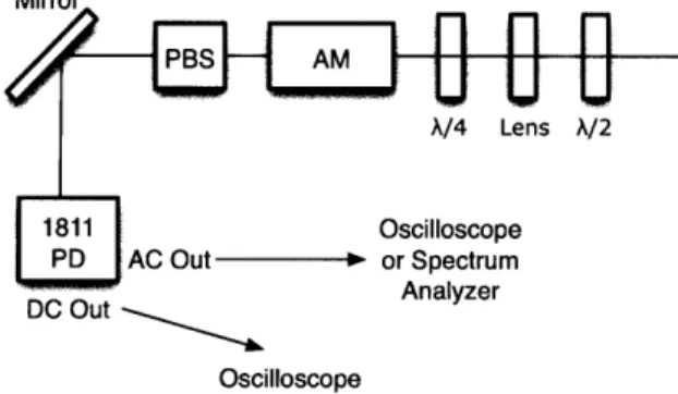
The goal of characterizing the New Focus amplitude modulator before and after modification was to ensure that the modifications required to convert the amplitude modulator to a UTM did not affect its ability to create pure amplitude modulation. Figure 6-1 shows the setup for the characterization of the New Focus 4104 amplitude modulator before and after modification.

To characterize the amplitude modulator before and after modification, the op-erating point where the amount of amplitude modulation was maximized had to be reached. (See appendix A for an alignment procedure.) This point, corresponding to half of the input power exiting the amplitude modulator, can be reached either by

Mirror

DC Out

Oscilloscope

Polarization Circular Vertical Output Intensity Minimum AM

T

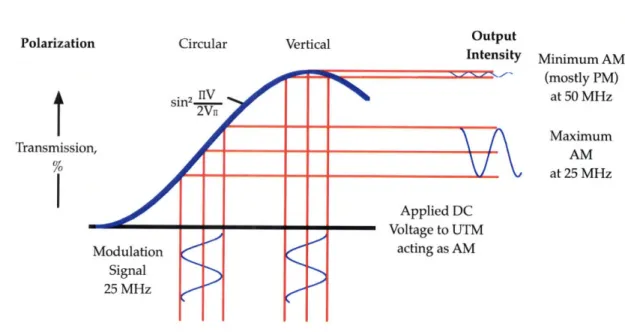
Transmissio: (mostly PM) at 50 MHz Maximum AM at 25 MHz

Figure 6-2: The amount of amplitude modulation is maximized with incident cir-cularly polarized light or with vertically polarized light incident and a DC (direct current) voltage such that the transmission percentage is half.

using a half- and quarter-waveplate in succession or using a half-waveplate and apply-ing a DC (direct current) voltage to the modulator's crystals. As shown in figure 6-2, positive and negative fluctuations in voltage as an applied modulation signal around this point cause decreases and increases, respectively, in the output intensity. This results in intensity, or amplitude modulation, at the modulation frequency. If instead of using circularly polarized light, the incident light is vertically polarized and no DC voltage is applied, the intensity modulation is at a minimum-the amplitude modu-lator is mostly outputting phase-modulation. The minimal intensity modulation will be at twice the modulation frequency because both positive voltage fluctuations cause a decrease in transmitted power. In figure 6-3 it is possible to see a signal at twice the modulation signal of 25 MHz when the incident light is vertically polarized. Figure 6-3 also illustrates that the modulation signal is maximized for circularly polarized light.

At the half power operating point, the modulation voltage to the amplitude ulator or UTM was varied and the resulting AC (alternating current) signal, or mod-ulation signal, was measured. The data and linear fits are shown in figure 6-4. The

E cL. 0 CL 10 15 20 25 30 35 40 45 50 55 60 Frequency [MHz] -20 E -30 -40 -50 0 -60 -70 80 10 15 20 25 30 35 40 45 50 55 60 Frequency [MHz]

Figure 6-3: Modulation signal with circularly polarized light (blue) and linearly verti-cally polarized light (red). The New Focus amplitude modulator (before modification) was driven with a 25 MHz signal in both cases. The blue curve corresponds to the operating point with half of the input intensity exiting the modulator. The red curve corresponds to a maximum of vertically polarized light out of the modulator. Thus, both the 25 MHz modulation signal and 50 MHz sideband are present.

I I I I I I I I

lO is 2o 2s 3o 3s 4o 45 so ss 6o

AM Characterization 1.4 1.4 1.2 1.2 c: c: s, s, >~0.8 >g0.8 U U 0 _e...

--->~0.6 >~0.6 U U <l: <l: 0.4 0.4 0.2 0.2 0 0 0 3 4 0 AC~n(pp) UTM Characterization 3 4 AC~n(pp)

Figure 6-4: Plot of AC voltage (peak-to-peak) over DC voltage out of the amplitude modulator (left) and UTM acting as an amplitude modulator (right) versus the input voltage of the modulation signal (25 MHz). Data points with error bars shown in red are fit to a line shown in blue.

slope of the fit line for the amplitude modulator is 0.195 ± 0.005 [l/V] and the inter-cept is given by -0.017

±

0.013. The slope of the fit line for the UTM is 0.200

±

0.005 [l/V] and the intercept is given by -0.003 ± 0.012. The slopes of these two lines, since they are one standard deviation apart, are consistent with the supposition that the ability of the ew Focus amplitude modulator to produce amplitude modulation was unchanged with the modifications required to convert it to a UTM.

Chapter 7

Data Analysis

7.1

Results

Error signals, as shown in figures 7-1, 7-2, and 7-3, were collected for three modulation states: nearly amplitude modulation, nearly phase modulation, and a combination of amplitude and phase modulation. For each error signal, the corresponding cavity transmission is also shown. While originally measured and fit in units of time, the x-axis units for each of the plots have been converted to units of cavity linewidths, or FWHMs (see equation 2.4), from resonance. The error signals were fit to the calculated error signal for arbitrary amounts of amplitude and phase modulation in order to fit for the fractions of amplitude and phase modulation. The calculated error signal can be derived using a procedure similar to that outlined in section 4.1 and is given by

!,[2A(-iDAM + DpM) X (F(w)F*(w + win) + F(w)F*(w - Wm))] (7.1)

where A is the amplitude of the carrier, DAM is the depth of amplitude modulation, and DpM is the depth of phase modulation. As given by equations 2.3 and 4.2, the reflection coefficient for the confocal cavity used in this experiment near resonance is given by

- om 0.8u 0.6 0. 0.2-a dl Voltage

[V]

. Cavity linewidths -2 - 1 0 1 2 from resonance

Figure 7-1: Nearly amplitude modulation error signal (top) with cavity transmission shown (bottom). Measured signals are shown in black and fits in red.

----

:::-

i..- I I I r I I II·

m ~i

I/

Figure 7-2: Nearly phase modulation error signal (top) with cavity transmission shown (bottom). Measured signals are shown in black and fits in red.

Cavity linewidths from resonance -C -C A-Voltage

[V]

Cavity linewidths 6 8 10 12 from resonance -6 -4 -2 0 2 4 -14-12-10 * 3 1 ~ * I I g I

L.A Now=

i

don&.

a

= -0.4 0.3 0.2 G.1i Volt -8 -6 -4 -2 0 2 4 ige

'I

8 10 12 Cavity linewidths from resonance

Figure 7-3: Combination amplitude and phase modulation error signal (top) with cavity transmission shown (bottom). Measured signals are shown in black and fits in red.

-12 -10

I I . I n *

where c(1-R), i = i-1, w/2r = v is the laser frequency, and wo is the cavity's

resonant frequency. However, we are not varying the frequency of the incoming light, but rather the length of the cavity, which forces the resonant frequency of the cavity to change. This is equivalent to changing the frequency of the incoming light. However, we might rewrite the error signal as a function of time as follows

a[2A(-iDAM + DpM) x (F(t)F*(f(t + win/f)) + F(ft)F*(f(t - win/f)))] (7.3) where f [frequency/time] is the rate at which the resonant frequency of the cavity changes with time. Equation 7.3 is then fit to the data to obtain A, f,DAM, and DpM.

The fractions of amplitude modulation and phase modulation, respectively, are given by

DAM DpM

XAM DAMXPM - DPM (7.4)

DAM + DpM DAM + DpM

For the three operating points-nearly all amplitude modulation, nearly all phase modulation, and a combination of amplitude and phase modulation-the fractions of amplitude and phase modulation were calculated. The results, as shown in table 7.1, verify that the UTM can produce nearly amplitude modulation, nearly phase modulation, and combinations thereof.

The cavity transmission was also fit, as shown in figures 7-1, 7-2, and 7-3. Equation 2.2 gives the cavity transmission as a function of frequency. The same method used above was used to convert equation 2.2 to a function of time. The transmitted intensity as a function of time is therefore given by

Io

I = ( 4-d I2 (7.5)

1 + (c(lR))2 (f(t - wolf))2

where, again, f is the rate at which the resonant frequency of the cavity changes. Equation 7.5 was fit to obtain Io and f.

The error signals are systematically shifted below resonance. This systematic offset is easily visible in figure 7-1; the zero crossings of the amplitude modulation

Operating Point Trial 1 Trial 2 Trial 3 Average Standard Deviation Nearly AM XAM 0.953 0.963 0.971 0.962 0.009 Nearly PM XPM 0.936 0.934 0.909 0.926 0.015 AM/PM Combination XPM 0.627 0.664 0.652 0.648 0.018

Table 7.1: Fractions of amplitude and phase modulation for nearly amplitude, nearly phase, and combination amplitude and phase modulation operating points. Averages with standard deviations are shown.

Operating Point Trial 1 Trial 2 Trial 3 Average Standard Deviation Nearly AM 0.297 0.287 0.318 0.301 0.016 Nearly PM 0.237 0.192 0.231 0.220 0.024 AM/PM Combination 0.285 0.228 0.336 0.283 0.054 Table 7.2: Amount error

linewidths.

signals are shifted below resonance in units of cavity

error signal do not correspond to the same level in transmitted power. An amplitude modulation error signal ought to cross zero at two points equally off-resonance. These offsets, for each of the modulation states, measured in cavity linewidths, are shown in table 7.2. As such an offset would affect the locking point of the cavity, further work should include determining and eliminating the source of such offsets.

7.2

Discussion and Conclusions

These data show that it is possible to produce nearly pure amplitude and phase modulation, as well as combinations thereof. The phase modulation error signal

has a single zero crossing, allowing for on-resonance locking; the amplitude and the combination amplitude and phase modulation error signals have two zero crossings, allowing for off-resonance locking at one of two points. Locking was achieved for each of such errors signals shown in figures 7-1, 7-2, and 7-3.

Additionally, the alternate method of using a test cavity and error signal fits to measure the amounts of amplitude and phase modulation was verified. Cusack et al. directly measured the amounts of amplitude and phase modulation. However, the cavity method allows for the confirmation of suitable error signals for on- and off-resonance locking of Fabry-Perot cavities.

Future work includes implementing the UTM into existing experiments in Prof. Mavalvala's lab. Such work includes optically integrating the UTM into existing setups as well as implementing remote computer control of the relative phases and amplitudes of the UTM's two crystals.

Appendix A

UTM Alignment Procedure

The following procedure is used to align the UTM. Figure 6-1 shows a schematic 1. Without the quarter waveplate, maximize the power coming out the UTM after

the PBS adjusting the rotation of the half waveplate. Measure the power using the power meter.

2. Adjust the screws on the AM mount to maximize the power coming out the the AM before the PBS. Measure the power using the power meter.

3. Place the power meter after the PBS. Maximize the linearly polarized power by adjusting the screws on the AM mount and by moving the knob on the half waveplate. Treat the knob on the half waveplate as a fifth screw.

4. Now apply a 25MHz voltage signal to the UTM. Observe how the AC and DC signals out of the photodetector (an 1811) change as the rotation of the alignment mirror. Maximize the DC power to the 1811. Ideally, there should be no AC signal. If this isn't the case, adjust the rotation of the mirror such that it is. This is the maximum power operating point, which was recorded on the spectrum analyzer as shown in figure 6-3.

5. Now, place the quarter waveplate in the beam path, as shown in figure 6-1. (When rotating the alignment mirror, I would sometimes notice that the AC voltage would increase while the DC voltage decreased. I'm not really

sure how to explain this, although when I replaced the quarter waveplate the effect was lessened.) Rotate the quarter waveplate such that the DC power is halved. As you rotate the quarter waveplate past this point, the power should increase. That is, half the power should be the minimum. Also, power should be halved to maximize the AC signal. If this is not the case, repeat the alignment process. This is the half power operating point (or maximum modulation operating point) and was recorded on the spectrum analyzer as shown in figure 6-3.

Appendix B

UTM Notes

The prototype UTM built by modifying an amplitude modulator. To convert an amplitude modulator to a UTM, the amplitude modulator is modified such that the two perpendicularly aligned LN crystals are driven by two independent signals instead of just one. By varying the phase between the crystals' signals, the relative amounts of AM and PM can be controlled. I wanted to figure out whether it was possible to use only one lithium niobate crystal and, if so, if there were advantages to using two crystals instead of one.

The index ellipsoid for a lithium niobate crystal in an electric field E = (E., Ey, Ez) is

1 = + r13Ez - r22Ey) X2 l+ T'13Ez + r22Ey) Y2 + r33Ez) Z4B.1) +2r42EyXY + 2r42ExYZ + 2r22ExXZ (B.2)

where rij (m/V) is the tensor which describes the linear electrooptic effect for lithium niobate, no,, is the index of refraction along the ordinary axes, and ne is the index of refraction along the extraordinary axis of the crystal. Here, the coordinates X, Y, and Z do not define the principle axes of the crystal in the presence of an electric field. To find the principle axes and the corresponding indices of refraction along

these axes, we begin by writing the index ellipsoid in terms of vectors and matrices: 11

(

+ r1₃Ez - r₂₂Ey r42Ey r22Ex

X

n = X

Y

Z r42EY 1 +ri3Ez

+r

22Ey r42Ex Y r22Ex r42Ex 2 + r3aEz Z (B.3)

The eigenvalues and eigenvectors of the 3 x 3-matrix will give the indices of refraction and the principle axes of the crystal with an electric field present. If we set Ex = 0, the eigenvectors do not depend on the applied electric field. This means that as we vary the electric field, the principle axes of the ellipsoid do not change. (If Ex j 0, the eigenvectors do depend in the electric field. This gives rise to a far more complicated situation.) The new (unnormalized) principle axes in the case of Ex = 0, Ey 5 0

and Ez

$

0 are given by

x= YZ r22+r r ₂ T 2 1

1042

0 (B.4)

y=

(

Y

Z

)(

-r22+ 1 0 (B.5)

r42

z = Z. (B.6)

The corresponding indices of refraction along these axes are given by one over the square root of the eigenvalue. This yields (to first order)

r13Ez-iv2 T 2 Ej

nx = no 213Ez- Ey n3 (B.7)

riE n 2 _ Ey

n

no-

r 2

n3

(B.8)

n = ne - 3zn (B.9)

If we allow the light to propagate in the & direction the phase delay, F, between the

9 and ^ polarizations is given by

r 3aE 1 -22 r4nEY.2

F = (r33n - r13no)Ez - r 2 + r 2nEy. (B.10)

arbitrary amounts of amplitude and phase modulation with a single crystal.

It is now clear that there are a couple of reasons that two crystals are used instead of one. First of all, the geometry of the one-crystal-situation is somewhat tricky. It would be far simpler to only apply an electric field in the Z-direction, since the principle axes would not change. Second, it is possible to show that when amplitude modulating with two lithium niobate crystals, the constant phase shifts due to thermal fluctuations in the length of the crystal are canceled out. When amplitude and phase modulating with the UTM, the two-crystal setup will also prevent problems with the amplitude modulation and a constant phase shift has no measurable effect on phase modulation.

Bibliography

[1] Benedict J Cusack, Benjamin S Sheard, Daniel A Shaddock, Malcolm B Gray, Ping Koy Lam, Stan E Whitcomb. Study of an electro-optic

modu-lator capable of generating simultaneous amplitude and phase modulations.

http://arxiv.org/abs/gr-qc/0306077, 2003.

[2] Saulson, Peter R. Fundamentals of Interferometric Gravitational Wave Detectors. World Scientific Pub Co. Inc., 1994.

[3] LIGO Scientific Collaboration, Ed. P. Fritschel. Advanced LIGO Systems Design. LIGO Technical Note, 2001.

[4] Corbitt, Thomas et al. Squeezed-state source using radiation-pressure-induced

rigidity. Physical Review A, 73, 2006.

[5] Corbitt, Thomas et al. Measurement of radiation-pressure-induced optomechani-cal dynamics in a suspended Fabry-Perot cavity. Physioptomechani-cal Review A, 74, 2006.

[6] Corbitt, Thomas et al. Toward achieving a low energy state of a gram-scale mirror

oscillator. http://arxiv.org/abs/0705.1018v1, 2007.

[7] Sinclair, D.C. Scanning Spherical-Mirror Interferometers for the Analysis of Laser

Mode Structure. Laser Technical Bulletin, Number 6. Spectra-Physics. 1968.

[8] Boyd, Robert W. Nonlinear Optics. Elsevier Science. San Diego, CA. 2003. [9] Yariv, Amnon. Quantum Electronics. John Wiley & Sons, Inc. New York, 1967.

[10] Black, Eric. Notes on the Pound-Drever-Hall Technique. LIGO Technical Note, 1998.