HAL Id: hal-02054190
https://hal.sorbonne-universite.fr/hal-02054190
Submitted on 1 Mar 2019HAL is a multi-disciplinary open access archive for the deposit and dissemination of sci-entific research documents, whether they are pub-lished or not. The documents may come from teaching and research institutions in France or abroad, or from public or private research centers.
L’archive ouverte pluridisciplinaire HAL, est destinée au dépôt et à la diffusion de documents scientifiques de niveau recherche, publiés ou non, émanant des établissements d’enseignement et de recherche français ou étrangers, des laboratoires publics ou privés.
Observations and Modeling
S. Dacie, T. Török, P. Démoulin, M. Linton, C. Downs, L. Van
Driel-Gesztelyi, M. Long, J. Leake
To cite this version:
S. Dacie, T. Török, P. Démoulin, M. Linton, C. Downs, et al.. Sequential Eruptions Triggered by Flux Emergence: Observations and Modeling. The Astrophysical Journal, American Astronomical Society, 2018, 862 (2), pp.117. �10.3847/1538-4357/aacce3�. �hal-02054190�
TEX preprint2 style in AASTeX61
SEQUENTIAL ERUPTIONS TRIGGERED BY FLUX EMERGENCE - OBSERVATIONS AND MODELING
S. DACIE,1 T. T ¨OROK¨ ,2P. D ´EMOULIN,3M. G. LINTON,4 C. DOWNS,2 L.VANDRIEL-GESZTELYI,1, 3, 5
D. M. LONG,1 ANDJ. E. LEAKE6
1Mullard Space Science Laboratory, University College London, Holmbury St. Mary, Surrey, RH5 6NT, UK 2Predictive Science Inc., 9990 Mesa Rim Road, Suite 170, San Diego, CA 92121, USA
3Observatoire de Paris, LESIA, UMR 8109 (CNRS), F-92195 Meudon-Principal Cedex, France 4Naval Research Laboratory, Washington, DC 20375, USA
5Konkoly Observatory of the Hungarian Academy of Sciences, Budapest, Hungary 6NASA Goddard Space Flight Center, 8800 Greenbelt Rd, Greenbelt, MD 22071, USA
ABSTRACT
We describe and analyze observations by the Solar Dynamics Observatory of the emergence of a small, bipolar active region within an area of unipolar magnetic flux that was surrounded by a circular, quiescent filament. Within only eight hours of the start of the emergence, a partial splitting of the filament and two consecutive coronal mass ejections took place. We argue that all three dynamic events occurred as a re-sult of particular magnetic-reconnection episodes between the emerging bipole and the pre-existing coronal magnetic field. In order to substantiate our interpretation, we consider three-dimensional magnetohydrody-namic simulations that model the emergence of magnetic flux in the vicinity of a large-scale coronal flux rope. The simulations qualitatively reproduce most of the reconnection episodes suggested by the obser-vations; as well as the filament-splitting, the first eruption, and the formation of sheared/twisted fields that may have played a role in the second eruption. Our results suggest that the position of emerging flux with respect to the background magnetic configuration is a crucial factor for the resulting evolution, while previ-ous results suggest that parameters such as the orientation or the amount of emerging flux are important as well. This poses a challenge for predicting the onset of eruptions that are triggered by flux emergence, and it calls for a detailed survey of the relevant parameter space by means of numerical simulations.
Keywords:Sun: magnetic fields – Sun: corona – Sun: coronal mass ejections (CMEs)
Corresponding author: Tibor T¨or¨ok [email protected]
1. INTRODUCTION
Coronal mass ejections (CMEs) are eruptions of sheared or twisted magnetic fields from the solar corona. They may contain a filament consisting of dense and cool material initially suspended above the solar surface. Many mechanisms have been proposed to explain how CMEs (and associated flares) are initiated, causing the magnetic struc-ture to rise (see, e.g.,Aulanier 2014). At a critical height, the structure is believed to become torus unstable (Kliem & T¨or¨ok 2006), which causes it to rapidly accelerate upward. At the same time, a current sheet forms between oppositely orientated field lines beneath the unstable structure. Recon-nection within the current sheet leads to flaring (as in the CSHKP model Carmichael 1964; Sturrock 1966; Hirayama 1974; Kopp & Pneuman 1976) and additional acceleration of the ejecta.
One possible mechanism for the initiation of eruptions is flux emergence nearby a preexisting, current-carrying magnetic structure, as described by, e.g., Chen & Shibata (2000). In their simula-tion labeled as case B, bipolar field emerges near to a flux rope that is in stable equilibrium with the am-bient field. The new flux is orientated “favorably” for reconnection, as defined byFeynman & Martin
(1995), meaning that the orientation of the emerg-ing bipole is chosen such that a current layer forms between the flux rope and the bipole. As recon-nection occurs across the current layer, two new sets of field lines are created; a small arcade that connects the emerging flux and the ambient field, and long field lines that arch over the flux rope and connect to the other polarity of the emerging flux (see Figures 5b inChen & Shibata 2000and 3a in
Williams et al. 2005). These latter field lines be-come somewhat longer due to the displacement of one of their foot points, so their downward acting magnetic tension decreases. This ongoing reduc-tion of magnetic tension leads to a continuous slow rise of the flux rope, which finally leads to loss of equilibrium (or torus instability) and the eruption of the rope. The eruption is potentially facilitated
also by an overall expansion of the ambient field due to the changes in the photospheric flux distri-bution (Ding & Hu 2008).
There have been many observational studies of newly emerging flux occurring before CMEs (Feynman & Martin 1995;Wang & Sheeley 1999;
Jing et al. 2004; Xu et al. 2008; Schrijver 2009). These have shown that the most favorable condi-tions for triggering a CME arise when the orien-tation of the emerging flux is opposite to that of the existing field and when the emergence occurs close to the polarity inversion line (PIL; e.g., Xu et al. 2008). However, Louis et al. (2015) associ-ated a flare and CME with flux emergence that was neither of favorable orientation nor located close to the PIL, and other exceptions can be found in the studies mentioned above. Other observations have shown magnetic flux emergence apparently causing a filament to split (Li et al. 2015). These contrasting observations suggest that the set of conditions required for emerging flux to initiate an eruption are not yet fully understood (see alsoLin et al. 2001).
Many modeling studies have been able to pro-duce eruptions by introducing emerging flux into a pre-existing magnetic field configuration; either containing a potential or sheared arcade field ( No-toya et al. 2007;Zuccarello et al. 2008, 2009; Ku-sano et al. 2012; Jacobs & Poedts 2012; Roussev et al. 2012;Kaneko & Yokoyama 2014), or a flux rope (e.g. Chen & Shibata 2000; Lin et al. 2001;
Xu et al. 2005; Shiota et al. 2005; Dubey et al. 2006; Ding & Hu 2008). Whether an eruption is produced depends on various parameters such as the strength of the new magnetic flux and its po-sition and orientation. Changing these parameters can lead to cases where the emerging flux acts to additionally stabilize a flux rope rather than trig-gering its eruption (e.g. the cases shown in Figure 7 ofChen & Shibata 2000).
In this paper, we study the effects of the emer-gence of a small bipole nearby a quiescent circular filament on 18 July 2014. The eastern section of
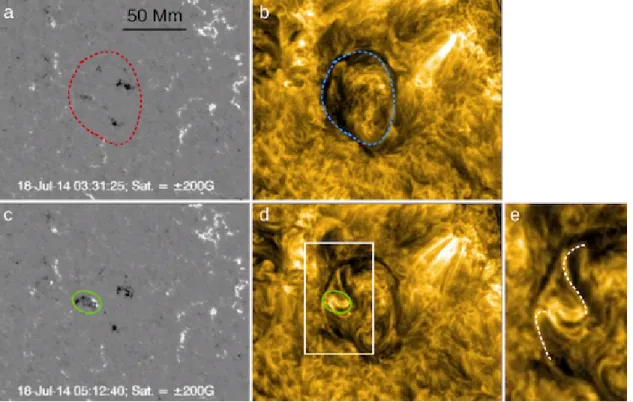
Figure 1. Apparent splitting of the eastern section of the filament. Length scales for panels (a)–(d) are indicated in (a). Shown are HMI magnetograms (left) and AIA 171 ˚A images (right), at 03:30 UT (top) and 05:12 UT (bottom) on 18 July 2014. (a) Magnetogram and (b) quiescent filament around the onset of emergence. Red (blue) dashed lines outline the filament location. (c) Region of flux emergence (green oval), slightly to the west of the eastern filament section. (d) Interaction between emerging flux and pre-existing magnetic field. Bright streaks reach both northward and southward, suggesting new magnetic connectivities. (e) Zoom into the area shown as white rectangle in (d). White dashed lines outline the new connectivities. The AIA images shown here and in Figure4were processed using the Multi-scale Gaussian Normalization Technique ofMorgan & Druckm¨uller(2014). An animation of this figure is available with the online version of this manuscript.
the filament is seen to partially split and to form new connectivities, followed by the eruption of its western section shortly after. A few hours later, a second eruption occurs above the PIL segment that has formed between the emerging flux and the pre-existing field, suggesting the formation of non-potential magnetic fields at this location during the emergence of the bipole. In Section2, we discuss the observations and propose mechanisms to ex-plain these activities. In Section3we present mag-netohydrodynamic (MHD) numerical simulations that qualitatively reproduce the filament splitting and the first eruption, and suggest a possible mech-anism for the formation of a flux rope between the emerging and preexisting flux. Finally, we discuss the results and draw our conclusions in Section4.
2. OBSERVATIONS AND PROPOSED MECHANISMS
2.1. Data
A quiescent circular filament and the newly forming active region NOAA 12119, which emerged within a negative polarity area encircled by the fil-ament, close to its eastern section, were studied for the eight hours following the start of the active region’s emergence at ≈ 03:30 UT on 18 July 2014 at [-376”, -415”] in helioprojective-cartesian coor-dinates. The partial splitting of the filament and the two eruptions occurred during this time period. Data from the Atmospheric Imaging Assembly (AIA;Lemen et al. 2012) on board the Solar Dy-namics Observatory (SDO; Pesnell et al. 2012) were used to identify structures and
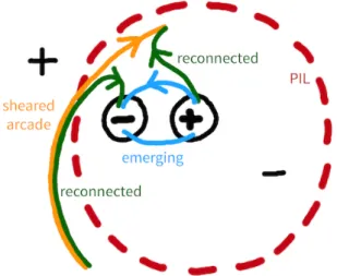
connectivi-Figure 2. Diagram showing the splitting mechanism. The red dashed circle represents the PIL of the pre-emergence magnetic configuration, above which the fil-ament resides (Figure1(b)). The emerging bipole is sketched with + and - signs in black circles, and blue field lines representing its magnetic connectivities. The orange line, which crosses the PIL, represents a highly sheared field line of the eastern filament arcade. It re-connects with the emerging bipole, forming the green field lines.
ties in the corona, and photospheric line-of-sight magnetic field measurements, provided by the He-lioseismic Magnetic Imager (HMI; Schou et al. 2012) were used to calculate the magnetic flux of the emerging bipole. All images shown in Figs.1
and 4 below were rotated to the observer’s view at 05:55 UT on July 18, which is roughly midway between the respective onset times of the partial filament splitting and the first eruption. The center of this field of view is at -23.7◦ longitude (in heli-ographic coordinates). We refrained from rotating all images to the central meridian, to minimize the interpolation of the data.
2.2. Splitting of the Eastern Filament Section The quiescent filament (shown in Figure1(b) at 03:30 UT on 18 July 2014) was almost circular in shape and had formed between an area of dis-persed negative field (inside the dashed line shown in Figure1(a),(b)) and positive field (outside). An emerging bipole, which later becomes active re-gion NOAA 12119, began to emerge just to the
west of the eastern section of the circular filament. The orientation of its magnetic fields is mostly West to East, although the presence of magnetic tongues leads to some deviation of the PIL orien-tation from that direction (Figure1(c)). Following
Poisson et al.(2016), these tongues are interpreted as the contribution of the azimuthal field compo-nent of the emerging flux tube. They indicate a negative magnetic helicity, which is also suggested by the shear of the loops seen in the corona (Figure
1(d)).1
As the new flux started to emerge, it immediately began to interact with the surrounding magnetic field, as is apparent from the formation of bright loops in the AIA 171 ˚A images as early as 05:12 UT. These loops are shown in Figure1(d) and out-lined by dashed white curves in the zoom shown in panel Figure1(e). They are indicative of new magnetic connectivities as a result of reconnection between the magnetic field of the emerging bipole and the magnetic structure supporting the filament, which is likely a highly sheared arcade.
Figure2is a top-down diagram showing the field lines of the sheared arcade before reconnection (or-ange), those of the emerging bipole (blue), and those formed by reconnection (dark green), which are of the same shape as the bright loops outlined in Figure1(e). This reconnection likely causes the sheared arcade (and thus the filament) to split, at least partially, with some of its flux becoming con-nected to the emerging bipole.
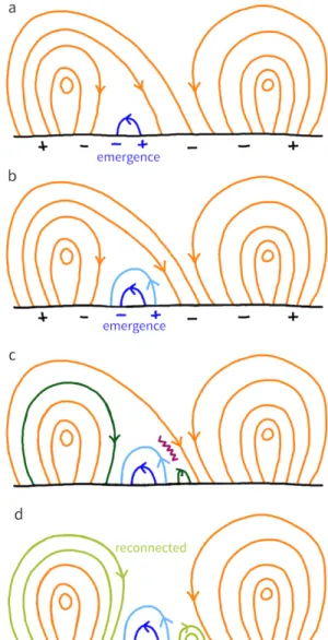
A schematic side-on view of this phase of the evolution is shown in Figure3, emphasizing recon-nection of the emerging bipole with the field sur-rounding the highly sheared filament-arcade core. Here again, the orange field lines depict the fila-ment arcade, blue depict the emerging bipole and green those formed by reconnection. Since the field lines are drawn on a 2D plane, those of the
1Luoni et al.(2011) showed that the helicity sign derived
from a magnetic-tongue pattern agrees with other proxies, such as loop shear.
emerging bipole and those surrounding the core of the eastern filament arcade appear to be oriented parallel to each other, but this is not the case in re-ality.
The dark green field line on the left of Figure3(c) is equivalent to that on the left of Figure 2. This field line has been shortened by the reconnection (see Figure2), which increases its magnetic ten-sion and leads to an additional stabilization of the core field. The small dark green line of Figure3(c) is equivalent to the smaller reconnected line shown in Figure 2. In what follows, we refer to the new magnetic connection associated with the latter line as the “new arcade”. Since the new arcade forms by reconnection between the bipole and the origi-nal filament arcade, it likely contains a significant amount of shear/twist, which may have been re-quired for powering the second eruption described below.
Due to plasma heating caused by reconnection, it is difficult to follow the evolution of the fila-ment material involved in this reconfiguration. It appears that some of it ended up in the new ar-cade, as the observations show the presence of a north-south directed, S-shaped filament section that seems to follow that structure (Figures1(e) and 4), albeit some filament material may have been present at that location prior to the emergence (Figure1(b)).
2.3. First Eruption
The western part of the filament is seen to start rising slowly at ≈ 07:00 UT. Around 07:45 UT, the rise accelerates and the western part of the fila-ment fully lifts off. It erupts strongly non-radially eastward, over the eastern part of the filament, and seems to drag the latter with it. It thus appears that the whole filament erupts (Figure4(e)), except per-haps those sections that were disconnected during the earlier phase of the bipole emergence. The flare loops produced by this eruption can be clearly seen in AIA 171 and 193 ˚A images, as shown in Figure
4(e),(f). The CME associated with this eruption is first seen in data from the Large Angle and
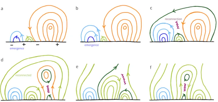
Spec-Figure 3. 2D diagram showing the reconnection de-scribed in Section2.2. The black line indicates the pho-tosphere. Dark (light) blue field lines represent newly emerging flux (emerged in the previous panel). Orange field lines show a cross-section of the pre-existing field configuration; with the eastern (western) filament ar-cade on the left (right). Dark (light) green field lines are formed by reconnection (reconnected in the previ-ous panel). The purple zigzag line represents a current sheet where reconnection takes place. The reconnection produces two new field-line sets, anchored in the nega-tive and posinega-tive polarity of the bipole, respecnega-tively (cf. Figure2). Note that new flux continues to emerge in panels (c) and (d), but is omitted for clarity.
trometric Coronagraph (LASCO; Brueckner et al. 1995) C2 on board the Solar and Heliospheric Ob-servatory(SOHO) at ≈ 09:35.
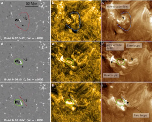
Figure 4. First and second eruption. The length scales for all panels is indicated in (a). Shown are HMI magnetograms (left), AIA 171 ˚A (center) and 193 ˚A (right) images. (a)–(c) Before the first eruption, at 07:04 UT on 18 July 2014. Dashed lines indicate the location of the filament that undergoes the first eruption. The bright new arcade field lines in (c) are formed by reconnection of the emerging flux with the pre-existing filament arcade, as shown in Figure5(c). (d)–(f) Shortly after the first eruption, at 08:59 UT. The flare loops produced in the eruption can be seen in (e) and (f). The total unsigned magnetic flux of the emerging bipole was ≈ 4.7 × 10²⁰Mx, and it had a size of about 25 × 12 Mm
at this time. (g)–(i) Just after the second eruption, at 10:56 UT. The dashed lines indicate the PIL of the erupted arcade. Sheared flare loops produced in the eruption can be seen in (h) and (i). The flux-emergence region is outlined by green ovals in panels (d)–(i). At this time, the emerging bipole has reached a total size of about 28 × 13 Mm and a total flux of ≈ 6.0 × 10²⁰Mx. An animation of this figure is available with the online version of this manuscript.
The observations are interpreted as shown in Fig-ure 5(a)–(d) and described as follows. After the emerging bipole has ‘eaten through’ all of the field lines of the eastern arcade, it can start to reconnect with the western arcade. This reconnection (Fig-ure5(c)) produces two new sets of field lines (dark green); small loops and long overlying ones.
The bright loops seen in Figure 4(c) before the eruption are interpreted as these small loops, which connect the positive polarity of the emerg-ing bipole and the negative polarity of the filament arcade. They are expected to accumulate above the
sheared new arcade that formed earlier on, during the reconnection between the emerging bipole and the eastern filament arcade (Figures2and3(c),(d)). The long overlying loops produced by the recon-nection shown in Figure5(c) have a lower mag-netic tension than the field lines that were over-lying the filament originally, allowing the western filament arcade to rise. At some point of the evolu-tion the magnetic configuraevolu-tion becomes unstable, possibly due to loss of equilibrium (or torus insta-bility) and erupts. Reconnection beneath the fila-ment (Figure5(d)) produces the western flare loops
shown in Figure 4(f). This is the same process as described in case B of Chen & Shibata (2000) for an eruption caused by flux emergence nearby a flux rope, and as demonstrated for a fully three-dimensional (3D) configuration in Section3.2.
After the eruption, flare loops can also be seen to the east of the emerging bipole (Figure4(f)). The observations indicate that the eruption of the western section of the filament likely destabilized the whole magnetic structure that overlies the PIL shown in dark red in Figure4(a), which appears reasonable since the highly sheared field carrying the filament was likely extending over the whole PIL. This means that the shortening of the field lines shown in Figure3(c),(d) was not sufficient to stabilize the configuration, which again appears reasonable as those field lines were relatively large. In this scenario, the eruption is expected to form loops along the entire length of the PIL, but not all of these are observed, probably due to differ-ences in the plasma density associated with the lo-cal amount of reconnected flux (less energy is lib-erated in weaker magnetic fields). As for the re-connection described in Section2.2, this 3D effect along the circular PIL cannot be depicted in the 2D cartoons of Figure 5, which represents only a 2D cut of the configuration on the western side of the emerging bipole.
2.4. Second Eruption
The second eruption originates above the new PIL between the positive polarity of the emerging bipole and a pre-existing negative flux concentra-tion (dashed red line in Figure4(g)). The eruption occurs just a few hours after the first eruption, at ≈ 10:30 UT. Bright flare loops are seen after this second eruption (Figure 4(h),(i)), showing the re-laxation of a highly sheared arcade over a period of about 25 minutes. The CME associated with the second eruption enters the LASCO C2 field of view at ≈ 11:50 UT. It appears to travel faster than the first eruption, which may be due to a removal of some of the overlying coronal field by the first eruption.
The magnetic structure that most likely powers the second eruption is the new arcade that was formed by the reconnection process described in Section2.2. It is indicated by the small green field lines on the right-hand side of the emerging bipole in Figure3(d). Magnetic flux is added to this new arcade during the reconnection that triggers the first eruption (Figure5(c)). The continuous west-ward motion of the leading positive polarity of the bipole towards the PIL of the new arcade likely concentrated the arcade’s shear. Additionally, a highly twisted flux rope may have formed beneath the arcade by the process described in Section3.3.
How is the second eruption initiated? As shown in Figure5(d), the first eruption leaves behind a region of reduced magnetic pressure, into which the sheared new arcade (or flux rope) can ex-pand. This induces reconnection between the ar-cade and the erupting flux to its right-hand side (Figure5(e)). Note that this reconnection works in the opposite direction as the earlier one shown in Figure5(c): rather than adding closed flux to the arcade, it opens up flux on its top, thereby re-ducing the magnetic tension that holds down the arcade’s sheared/twisted core. Such behavior has been previously observed, with flare ribbons mov-ing backwards well after a CME was launched: see Figures 11 and 12 inGoff et al. (2007) for a simi-lar reversal of the reconnection direction after the launch of a CME. This eventually facilitates the eruption of the core flux, which evolves into the second CME. Behind the eruption the reconnec-tion shown in Figure5(f) is induced, which creates the flare loops seen in Figure4(h),(i).
We note that the mechanism described here for the triggering of a second eruption due to a reduc-tion of magnetic tension by a preceding erupreduc-tion that occurs in an adjacent flux system is basically the same as modeled for “sympathetic” eruptions by T¨or¨ok et al. (2011) and Lynch & Edmondson
(2013); see also Gary & Moore (2004); DeVore & Antiochos (2005); Joshi et al.(2016); Li et al.
Figure 5. Same as Figure3, now for the mechanisms believed to produce the two eruptions. (a) Emerging bipole (blue), new arcade (green), and western filament-arcade (orange). The eastern filament-arcade does not participate in the evolution and is omitted here. (b) Continuing bipole emergence and expansion in the corona. (c) Reconnection between bipole and western filament-arcade, forming long overlying field lines and smaller loops above the new arcade. The lengthening of the overlying field lines reduces the magnetic tension on the western filament-arcade, allowing it to expand. (d) Eruption of the western filament-arcade and associated reconnection underneath the filament, cutting its ties to the photosphere and further accelerating it upwards. (e) Expansion of the new arcade induces reconnection with locally open field lines left behind from the eruption, accelerating its rise. (f) Second eruption and flare loops formed by the reconnection in the wake of the eruption.
3. NUMERICAL MODELING
In this section we compare our interpretations of the observations with MHD simulations of the emergence of a strong and compact bipole in the vicinity of a large coronal flux rope. The simu-lations we consider here are part of a parametric study that was performed to study the triggering of CMEs by flux emergence (as observed and an-alyzed by, e.g., Feynman & Martin 1995). This study will be described in a forthcoming publica-tion (T¨or¨ok et al., in preparapublica-tion); here we restrict ourselves to a brief description of the basic setup.
We emphasize that the simulations of our para-metric study were not designed to reproduce the event analyzed in Section2, which results in a number of differences between the simulations and the observations (see below). Specifically, we are not intending here to reproduce the whole chain of the observed dynamic events (filament
split-ting, first and second eruption) in a single simula-tion. Rather, we choose from our parametric study three independent simulations that start from the same initial state and differ only in the distance be-tween the pre-existing flux rope and the emerging bipole. Each simulation addresses only one of the observed dynamic events. Also, it should be kept in mind that the simulations use idealized config-urations, i.e., they are not intended for a quanti-tative comparison with the observations. Instead, they should be considered merely as “proof-of-concept”, serving to support our interpretations of the observations in terms of different reconnection processes and the resulting dynamics and system reconfigurations. We leave the design of a more re-alistic simulation of the observed events to a later investigation.
The simulations described here were performed using the MAS (Magnetohydrodynamic Algorithm
outside a Sphere) code (e.g.,Mikic & Linker 1994;
Lionello et al. 1999), which advances the stan-dard viscous and resistive MHD equations. The β = 0 approximation, in which thermal pressure and gravity are neglected, was used here, so that the evolution is driven by the Lorentz force. The use of this approximation is justified here, since the dynamics relevant for our investigation occur in corona, where the plasma beta is low. The spher-ical simulation domain covers the corona within 1.0–3.5 R , where R is the solar radius. We
note that, even though the lower boundary of the MAS domain is associated with the solar surface (r = R ), it should physically be considered here
as the bottom of the corona, since we use the β = 0 approximation.
The initial coronal magnetic field consists of a flux rope embedded in a bipolar AR, as shown in a top-down view in Figure6(a). This con-figuration was constructed using the modified Titov-D´emoulin model (TDm; Titov et al. 2014), such that the flux rope is initially in stable mag-netic equilibrium. The center of the TDm con-figuration is placed at the position (r, θ, φ) = (1., 1.125, 2.46), with r in units of R and θ, φ in
radians. The axis of the TDm flux rope is aligned with the φ axis.
After relaxing the system until a sufficiently ac-curate numerical equilibrium is obtained, the emer-gence of a strong, compact bipolar AR is modeled “kinematically” (i.e., boundary-driven). To this end, horizontal slices of all three components of the magnetic field and the velocity are extracted at regular time intervals from an MHD simula-tion that used the Lare3D MHD code (Arber et al. 2001) to model the emergence of a flux rope from the convection zone into a non-magnetized corona (Leake et al. 2013).2 The slices are extracted at a height of the Lare3D simulation domain that corresponds approximately to the middle of the
2 The simulation used here is very similar to the cases
“ND” and “ND1” described inLeake et al.(2013).
photosphere-chromosphere layer used in these simulations (see Leake et al. 2013). The veloc-ity components are directly imposed at the lower boundary of the MAS domain and used for the momentum equation in MAS. The radial magnetic field, Br(t), of the Lare3D simulation is
superim-posed for all slices on Br(r = R ) of the TDm
configuration. This superimposed component and the extracted tangential fields and velocities are then used to calculate the electric fields required for the induction equation in MAS (see Lionello et al. 2013for details).
An extensive parametric study of the resulting evolution was performed by varying the strength, location, and magnetic orientation of the emerging flux. Changing these parameters can change the interaction between the existing and emerging flux system. This leads in some cases to an eruption of the TDm flux rope (for similar studies see, e.g.,
Chen & Shibata 2000andKusano et al. 2012). In the simulations presented here, the bipolar AR emerges for about 1.5 hours at an almost constant rate of ≈ 5 × 10²⁰Mx h−1, after which the emer-gence gradually slows down. After 6 hours, when the emergence has essentially saturated, the total unsigned flux of the AR is ≈ 1.3 × 10²¹Mx, which is about 20 per cent of the total flux of the TDm configuration. At this time, the modeled bipole has reached a size of ≈ 50 Mm (see Figure6(c)).
We note that in our simulations the orientation of the polarity centers changes in the course of the emergence from east-west to north-south, which can be best seen by comparing panels (a) and (b) of Figure8. This was not the case for the real bipole, which essentially maintained an east-west orientation throughout the whole observed evolu-tion. This indicates that the twist of the simulated emerging flux is larger than the twist of the real one. We believe that this difference does no affect the essential nature of the reconnection processes described in this section.
The polarity signs of the magnetic configura-tion and the handedness of the TDm flux-rope
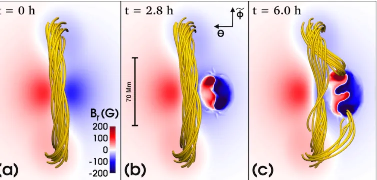
Figure 6. Simulation 1: Emergence of a bipolar flux region close to a pre-existing coronal flux rope. (a) Prior to emergence. Orange field lines depict the core of the TDm rope, which mimics the eastern section of the circular filament shown in Figure1. (b) Early emergence. Emerging and TDm-background field lines and the current layer that forms between the emerging and pre-existing flux systems are omitted for clarity (see Figures7and8). (c) Later emergence. Reconnection between the emerging flux and the TDm rope has led to the formation of new connectivities similar to the observed ones (cf. Figure1(e)). Length scales and coordinates are shown in (b).
were chosen in the parametric study without knowledge of the observed event described in this paper, and it turned out that they are oppo-site to those observed. Thus, when preparing the simulation data for the visualizations shown in Figures6–8, we generated an inverted coor-dinate, ˜φ (see Figure6(a)), by mirroring the φ coordinate about φ = 2.46 (the center of the TDm configuration). The φ-mirroring transforms the magnetic field from [Br(φ), Bθ(φ), Bφ(φ)] to
[(Br( ˜φ), Bθ( ˜φ), −Bφ( ˜φ)], keeping ∇ · B = 0 and
reversing only the φ component of the Lorentz force. This transformation changes the handed-ness of the TDm flux rope and of the emerging flux from negative to positive and from positive to negative, respectively, in agreement with the ob-servations. We finally reverse the sign of B, in order to reproduce the signs of all observed polar-ities. A corresponding procedure was applied to the current density, j, which is used in Figures7
and 8. These transformations do not affect the
evolution of the system, but significantly ease the visual comparison of the simulation results with the observations.
3.1. Splitting of the TDm Flux Rope We first consider the simulation shown in Fig-ure6, which we call “simulation 1” for further ref-erence. In this run, the bipole emerges centered around (r, θ, φ) = (1., 1.08, 2.46), close to the TDm flux rope (at a distance of 0.045 R in the θ
direction), within the negative polarity of the TDm background field. This qualitatively corresponds to the situation shown in Figure1, namely to the emergence of the bipole close to the eastern sec-tion of the circular filament. The orientasec-tion of the emerging flux in the simulation is such that the ini-tial axial-field direction of the emerging flux rope is antiparallel to the axial field at the core of the TDm flux rope.
Due to the vicinity of the emerging flux to the TDm rope, the two flux systems start to interact
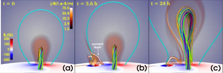
Figure 7. Simulation 2: Flux-rope eruption triggered by emerging flux. Here the TDm flux rope mimics the western section of the circular filament-arcade, so that in this view ˜φ points towards the viewer and θ to the right (cf. Figure6). Shown are the core of the TDm rope (rainbow-colored field lines), an overlying field line (cyan), and electric currents in a transparent vertical plane perpendicular to the TDm rope axis (shown by |j|/|B| in orange-white colors). (a) Initial configuration. The overlying field line is calculated starting from the positive (red) polarity of the TDm background field. (b) 3.6 h later, after a substantial amount of flux has emerged. The overlying field has expanded and its negative (blue) footpoint has been displaced by reconnection in the current layer that separates the emerging flux from the background flux. (c) Configuration after 24 h, showing the TDm flux rope in the process of eruption.
early on in the evolution. Initially, only field lines of the potential field surrounding the TDm flux rope come into contact with the outer field lines of the emerging flux. Since the field direction of these flux systems is essentially antiparallel, a cur-rent layer similar to the ones shown in Figures7
and8 is formed between them. Driven by the ex-pansion of the emerging flux in the corona, recon-nection across this layer sets in. Once the outer flux regions have reconnected, the reconnection contin-ues, now involving inner flux regions of the emerg-ing bipole and the TDm flux rope.
Figure6(c) shows a situation at which a consid-erable fraction of the TDm flux rope has already reconnected to form new connections between the rope’s foot points and the polarity centers of the emerging bipole. Being a result of reconnection, the corresponding field lines should appear bright in emission, just as the two streaks highlighted in Figure 1(e). The morphological agreement be-tween those streaks and the simulated new connec-tivities supports our interpretation that the emer-gence of the bipole resulted (at least partially) in the splitting of the flux rope or arcade that was
car-rying the eastern section of the circular filament (see Section2.2).
Due to the initial north-south orientation of the emerging flux rope in the simulation, the field lines of the TDm flux-rope core and of the core of the emerging flux rope are oriented essentially antiparallel when they come into contact and re-connect (Figure6). This was not the case in the observed event, where the corresponding field di-rections were approximately perpendicular to each other. Such an orientation should, however, still allow a reconnection of the type shown in Fig-ure6(c) to occur, as long as the interacting field lines are not close to being parallel (e.g., Linton et al. 2001). Indeed, in another simulation of our parametric study (not shown here), in which the orientation of the emerging flux rope was rotated by 3 π/8 (56◦) clockwise compared to simulation 1, we still found strong reconnection between the bipole and the TDm rope and the development of new connectivities very similar to those shown in Figure6(c).
Our second simulation (simulation 2) is shown in Figure7. In this simulation, the TDm flux rope represents the western section of the circular fil-ament. The orientation of the emerging bipole is the same as in simulation 1, but its center is now located at (r, θ, φ) = (1., 1.04, 2.46), about twice further away (0.085 R in the θ direction)
from the TDm rope (just outside of the negative flux concentration of the TDm background field). The larger distance reflects the fact that in the ob-served case the western filament section was fur-ther away from the emerging bipole than the east-ern section. The initial configuration of the simula-tion is shown in panel (a), where the cyan field line represents the potential background field overlying the TDm flux rope. As can be seen in panel (b), the emerging polarities and the TDm background po-larities together form a quadrupolar polarity pat-tern, corresponding to what Feynman & Martin
(1995) termed “favorable for reconnection”. Note that the view in the figure is chosen such that the bipole emerges to the left (to the east) of the flux rope, as it was the case in the observations.
As the new flux emerges, a current layer forms between the emerging flux and the TDm back-ground field. Reconnection across this layer dis-places field-line foot points of the background field from the edge of the negative TDm background po-larity to the negative popo-larity of the emerging flux, i.e., further away from the TDm flux rope (Fig-ure7(b)). The length of those field lines thus in-creases and they start to expand, which reduces the magnetic tension above the TDm rope.
However, reconnection is not the only mecha-nism leading to such expansion. As numerically demonstrated byDing & Hu(2008), adding a small bipole to a 2D flux-rope configuration changes the configuration in such a way that the magnetic field overlying the flux rope is more expanded, as long as the bipole is placed close to the rope and in an orientation “favorable for reconnection”. The ex-pansion is merely due to the change in the bound-ary condition of the system (see alsoWang &
Shee-ley 1999); reconnection is not required. This ef-fect takes place in our simulation, as the slowly emerging flux changes the boundary conditions of the coronal magnetic field. Due to the relatively large Alfv´en speed in the corona, this information has sufficient time to travel into the domain and to affect the coronal magnetic field.
The combined action of these two mechanisms is visualized in Figure7(b): the cyan field line has just reconnected with the emerging flux (see the strong kink of the field line at the position of the current layer), and its foot point on the left-hand side of the TDm rope has been displaced further away from the rope. Note that the field line has already expanded at the time it reconnects. This is partly due to the changes at the boundary, and partly due to the fact that field lines above it have reconnected and expanded earlier in the evolution. As a result of the continuous weakening of the magnetic tension due to field-line expansion, the TDm flux rope eventually cannot be stabilized any-more and erupts (Figure7(c)). The top of the rope rotates clockwise (when viewed from above), due to its right-handed twist (e.g., Green et al. 2007;
T¨or¨ok et al. 2010). Note that the initial opposite axial-field directions of the emerging flux rope and the TDm rope do not fundamentally affect the evo-lution in this case, since the TDm rope starts to erupt before it would significantly reconnect with the emerging flux.
In the simulation, the eruption sets in about one day after the beginning of the flux emergence, which is much later than in the real event, where the time difference was about four hours. The on-set time of the eruption depends on various param-eters, predominantly on “how far” the TDm rope is initially from an unstable state, and how efficiently the emergence and associated reconnection act in weakening the stabilizing tension of the overlying flux. Changing the strength and position of the emerging flux and/or changing the initial current in the TDm rope will lead to different onset times.
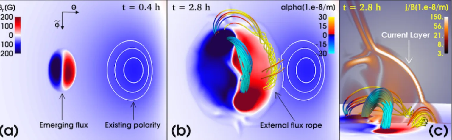
Figure 8. Simulation 3: emergence of a bipolar flux region close to a pre-existing flux concentration (similar to the observations shown in Figure4). The orientation of the configuration is the same as in Figure7; only the area containing the negative polarity of the TDm background field is shown. For better visibility, this polarity is highlighted by contour lines of -70, -80, and -90 G in panels (a) and (b). (a) Early phase of emergence. (b) 2.4 hours later. Field lines connecting the emerging-polarity centers outline the core of the emerging flux rope (cyan). A new flux rope has formed at the external PIL between the bipole and the pre-existing flux concentration (yellow). Field lines are colored by the force-free parameter α = j · B/B2; note that the two ropes have opposite handedness. Some arcade-like field lines (with smaller |α|) are shown above the new flux rope. (c) Tilted view of panel (b) along the PIL, showing additionally |j|/|B| in a transparent vertical plane.
To summarize, simulation 2 demonstrates that the scenario illustrated in Figure5(a)–(d), and modeled in 2D for an infinitely long flux rope by
Chen & Shibata(2000), can work also in fully 3D simulations, in which the foot points of the coronal flux rope are anchored in the photosphere. Thus, the simulation supports our interpretation put for-ward in Section2.3, namely that the first eruption was caused by a reduction of magnetic tension above the western part of the filament, as a result of flux emergence with an orientation “favorable for reconnection”.
3.3. Flux-Rope Formation Before Second Eruption
As described in Section2.4, the second erup-tion originates from the PIL that forms between the positive polarity of the emerging bipole and a neighboring, pre-existing negative flux concen-tration (Figure4(g)). In order for the eruption to occur, the flux residing above this PIL must have been non-potential. Since we found no indica-tions for the presence of a PIL at this location prior to the emergence of the bipole, the
correspond-ing shear/twist must have accumulated durcorrespond-ing the emergence process.
We suggested in Section2.4 that a new sheared arcade formed at this location by the reconnection process described in Section2.2, and that the shear further concentrated due to the westward motion of the positive polarity. However, it is not clear whether sufficient shear to power an eruption can build up solely by this process. In this subsec-tion we suggest an addisubsec-tional mechanism by which non-potential magnetic fields may have built up at this PIL. To this end, we consider a third simula-tion (simulasimula-tion 3). Note that we focus here only on the formation of the pre-eruptive structure; we do not aim to model the eruption itself.
In simulation 3, the orientation of the emerging flux is the same as in the previous simulations, i.e., the configuration is again “favorable” for recon-nection. The emergence is now centered around (r, θ, φ) = (1., 1.06, 2.46), at an intermediate dis-tance (0.065 R ) from the TDm rope (Figure8).
This simulation is intended to mimic the emer-gence of the observed bipole east of the existing negative flux concentration, shown in the left
pan-els of Figure4. We note that the formation of a new flux rope between the emerging and existing polar-ities, as described below, occurs in a very similar manner also in simulations 1 and 2. The reason why we use simulation 3 here to illustrate this pro-cess is that we had already analyzed that particular simulation regarding flux-rope formation prior to writing this article.
As in simulations 1 and 2, the expansion of the emerging flux in the corona leads to the forma-tion of a thin current layer (Figure8(c)). The layer develops above the “external” section of the PIL, i.e., the section that divides the positive emerg-ing polarity and the pre-existemerg-ing negative flux (Fig-ure8(a)). A complex dynamic evolution involving different types of reconnection in the current layer and downward directed flows leads to the forma-tion of a low-lying, highly twisted flux rope (Fig-ure8(b)). Note that this “external” rope is right-handed, while the less twisted, thicker flux rope that connects the polarity centers of the emerging flux is left-handed (seeLeake et al. 2013and refer-ences therein for the formation mechanism of this “central” flux rope).
The accumulation of twisted field lines above the external section of the PIL eventually ceases. However, reconnection in the current layer still continues, now producing sheared, arcade-type field lines that accumulate above the external flux rope (Figure8(b),(c)). This ongoing reconnection corresponds exactly to the one sketched in Fig-ure3(c),(d) and described in Section2.
The external flux rope forms in our simulation due to reconnection across the current layer in the corona, so the formation mechanism should be ro-bust with respect to the way in which the flux emer-gence into the corona is modeled (in our case via kinematic emergence). To check this, we have re-cently simulated an analogous situation using the Lare3D code, in which the flux emergence into a pre-existing coronal magnetic field is modeled dy-namically, i.e., though the buoyant rise of a flux rope through the convection zone. We found the
formation of an external flux rope also in this sim-ulation, which will be described in a forthcoming publication.
The mechanisms that lead to the formation of the external rope, the dependence of its formation and properties on parameters such as the amount of twist of the emerging flux, and the implications of this structure for coronal jets and filaments that form between active regions will be discussed in detail in a forthcoming publication (T¨or¨ok et al., in preparation). For our purpose, the important point is that the development of such a flux rope during the emergence of new flux in the vicinity of a pre-existing polarity provides an additional explana-tion for the presence of highly non-potential mag-netic fields along the PIL indicated by the dashed lines in Figures4(g)–(i).
4. SUMMARY AND CONCLUSIONS In this study, we investigated a magnetic config-uration in which a filament resided above a circu-lar PIL that encircled a dispersed negative pocircu-larity. We followed the early evolution of the small, bipo-lar active region NOAA 12119, which emerged within this polarity, close to the eastern section of the filament. Within eight hours of the onset of emergence, a partial splitting of the filament and two consecutive eruptions, both leading to CMEs, took place in the area. We utilized SDO data and MHD simulations to propose a scenario for the ob-served chain of events.
Based on the observations, we propose that the bipole initially emerges completely within the arcade-field overlying the eastern section of the filament. Reconnection of the two flux systems leads to a shortening of the field lines surrounding the core field of the filament arcade and stabilizes the core field in this area (Figures1(d),(e),2, and
3(c),(d)). This reconnection also causes at least a partial splitting of the field carrying the filament (similar to the case of Li et al. 2015) and thereby produces a new arcade (and S-shaped filament) that connects the bipole with the original filament.
After the western side of the emerging bipole has reconnected through the eastern arcade, it starts to reconnect also with the field of the western arcade (Figure5(c)). This reconnection adds flux to the previously formed new arcade. Simultaneously, it destabilizes the western arcade, allowing the west-ern section of the filament to rise and eventually erupt (Figures 4and5(d)).
Meanwhile, the continued emergence and west-ward motion of the leading polarity of the bipole may have concentrated the shear of the new ar-cade. Additionally, a highly twisted flux rope may have formed within it, as suggested by our simu-lation 3 (Section3.3). Since the first eruption has left behind a region of reduced magnetic pressure and weakened overlying field, the flux rope and surrounding new arcade can expand (Figure5(e)), eventually leading to the second eruption (as in the sympathetic eruptions modeled byT¨or¨ok et al. 2011).
Our simulations support this scenario. In sim-ulation 1 (Section3.1), a bipolar flux region is emerged within one of the polarities of the TDm background field, close to the location of the pre-existing flux rope. The emerging and pre-pre-existing TDm fields start to reconnect, and the TDm flux-rope field eventually forms new connectivities with the emerging bipole (Figure6(c)). The shapes and locations of these new connectivities correspond to the bright streaks seen in the observations (Fig-ure1(d),(e)), suggesting that they were indeed a re-sult of a partial splitting of the magnetic field car-rying the eastern section of the filament.
In simulation 2 (Section3.2), the bipole is emerged further from the TDm flux-rope and with an orientation such that a quadrupolar polarity pat-tern is formed. This setup mimics the interaction of the emerging flux with the western section of the filament. Both the changes in the boundary conditions caused by the emergence and reconnec-tion between the two flux systems act to reduce the tension of the field overlying the TDm flux rope, which eventually leads to its eruption. This
pro-vides an explanation for the first observed eruption, which begins in the western section of the circular filament, relatively far from the emerging bipole (Section2.3).
In simulation 3 (Section3.3), we model the for-mation of a highly twisted flux rope over the PIL between one polarity of an emerging bipolar flux region and a pre-existing flux concentration of op-posite polarity. This demonstrates that, in addi-tion to the new arcade, also a highly twisted flux rope may have formed in the source region of the observed second eruption. This addition of non-potential magnetic field may make it easier to un-derstand how the second eruption could originate in an area where concentrated sheared/twisted flux was not present prior to the flux emergence.
We conclude that the position of the emerging bipole with respect to the background magnetic field configuration is a crucial factor for the inter-action of these fields and the resulting evolution. Numerical simulations are able to qualitatively re-produce the various dynamic behavior observed for our case, and the upcoming study of T¨or¨ok et al. will help to characterize the relationship between the position of emerging flux (and of other pa-rameters such as its orientation, helicity sign, and amount of flux) and its interaction with the back-ground field (see also Kusano et al. 2012). Even relatively small amounts of emerging flux may be able to trigger significant changes in the coronal field, increasing the difficulty to predict eruptions. More systematic observations and parametric nu-merical simulation studies would give us a bet-ter idea of the conditions under which it should be possible to predict coronal activity triggered by flux emergence.
We thank the referee for thoughtful and inspir-ing comments and Ron Moore for a helpful dis-cussion regarding the second eruption. The au-thors are thankful to the SDO/ HMI and AIA con-sortia for the data. We also thank Z. Miki´c for assisting in coupling the Lare3D simulations to
MAS. S.D. acknowledges STFC for support via her studentship. L.v.D.G is partially funded under STFC consolidated grant number ST/N000722/1. L.v.D.G also acknowledges the Hungarian Re-search grant OTKA K-109276. D.M.L is an Early-Career Fellow funded by the Leverhulme Trust.
T.T, C.D, J.E.L, and M.G.L acknowledge support from NASA’s LWS and H-SR programs. M.G.L. acknowledges support from the Chief of Naval Re-search. We also thank the International Space Sci-ence Institute (ISSI) team 348 “Decoding the Pre-eruptive Magnetic Configuration of Coronal Mass Ejections” led by S. Patsourakos and A. Vourlidas.
REFERENCES
Arber, T. D., Longbottom, A. W., Gerrard, C. L., & Milne, A. M. 2001,Journal of Computational Physics, 171, 151
Aulanier, G. 2014,in IAU Symposium, Vol. 300, Nature of Prominences and their Role in Space Weather, ed. B. Schmieder, J.-M. Malherbe, & S. T. Wu, 184
Brueckner, G. E., Howard, R. A., Koomen, M. J., et al. 1995,Sol. Phys., 162, 357
Carmichael, H. 1964, in Phys. Sol. Flares, ed. W. N. Hess, 451
Chen, P. F., & Shibata, K. 2000,Astrophys. J., 545, 524
DeVore, C. R., & Antiochos, S. K. 2005,ApJ, 628, 1031
Ding, J. Y., & Hu, Y. Q. 2008, Astrophys. J., 674, 554 Dubey, G., van der Holst, B., & Poedts, S. 2006,
Astron. Astrophys., 459, 927
Feynman, J., & Martin, S. F. 1995,J. Geophys. Res., 100, 3355
Gary, G. A., & Moore, R. L. 2004,ApJ, 611, 545
Goff, C. P., van Driel-Gesztelyi, L., D´emoulin, P., et al. 2007,SoPh, 240, 283
Green, L. M., Kliem, B., T¨or¨ok, T., van
Driel-Gesztelyi, L., & Attrill, G. D. R. 2007,SoPh, 246, 365
Hirayama, T. 1974,Sol. Phys., 34, 323
Jacobs, C., & Poedts, S. 2012,SoPh, 280, 389
Jing, J., Yurchyshyn, V. B., Yang, G., Xu, Y., & Wang, H. 2004,Astrophys. J., 614, 1054
Joshi, N. C., Schmieder, B., Magara, T., Guo, Y., & Aulanier, G. 2016,ApJ, 820, 126
Kaneko, T., & Yokoyama, T. 2014,Astrophys. J., 796, 44
Kliem, B., & T¨or¨ok, T. 2006,Phys. Rev. Lett., 96, 1
Kopp, R. a., & Pneuman, G. W. 1976,Sol. Phys., 50, 85
Kusano, K., Bamba, Y., Yamamoto, T. T., et al. 2012,
Astrophys. J., 760, 31
Leake, J. E., Linton, M. G., & T¨or¨ok, T. 2013,ApJ, 778, 99
Lemen, J. R., Title, A. M., Akin, D. J., et al. 2012,Sol. Phys., 275, 17
Li, S., Su, Y., Zhou, T., et al. 2017,ApJ, 844, 70
Li, T., Zhang, J., & Ji, H. 2015,Sol. Phys., 290, 1687
Lin, J., Forbes, T. G., & Isenberg, P. A. 2001,J. Geophys. Res. Sp. Phys., 106, 25053
Linton, M. G., Dahlburg, R. B., & Antiochos, S. K. 2001,ApJ, 553, 905
Lionello, R., Downs, C., Linker, J. A., et al. 2013,ApJ, 777, 76
Lionello, R., Miki´c, Z., & Linker, J. A. 1999,Journal of Computational Physics, 152, 346
Louis, R. E., Kliem, B., Ravindra, B., & Chintzoglou, G. 2015,Sol. Phys., 1
Luoni, M. L., D´emoulin, P., Mandrini, C. H., & van Driel-Gesztelyi, L. 2011,SoPh, 270, 45
Lynch, B. J., & Edmondson, J. K. 2013,ApJ, 764, 87
Mikic, Z., & Linker, J. A. 1994,ApJ, 430, 898
Morgan, H., & Druckm¨uller, M. 2014,Sol. Phys., 289, 2945
Notoya, S., Yokoyama, T., Kusano, K., et al. 2007, in New Sol. Phys. with Solar-B Mission ASP Conf. Ser., Vol. 369, 381
Pesnell, W. D., Thompson, B. J., & Chamberlin, P. C. 2012,SoPh, 275, 3
Poisson, M., D´emoulin, P., L´opez Fuentes, M., & Mandrini, C. H. 2016,SoPh, 291, 1625
Roussev, I. I., Galsgaard, K., Downs, C., et al. 2012,
Nature Physics, 8, 845
Schou, J., Scherrer, P. H., Bush, R. I., et al. 2012,Sol. Phys., 275, 229
Schrijver, C. J. 2009,Advances in Space Research, 43, 739
Shiota, D., Isobe, H., Chen, P. F., et al. 2005,
Astrophys. J., 634, 663
Titov, V. S., T¨or¨ok, T., Mikic, Z., & Linker, J. A. 2014,
ApJ, 790, 163
T¨or¨ok, T., Berger, M. A., & Kliem, B. 2010,A&A, 516, A49
T¨or¨ok, T., Panasenco, O., Titov, V. S., et al. 2011,
Astrophys. J., 739, L63
Wang, Y.-M., & Sheeley, N. R., J. 1999,Astrophys. J., 510, L157
Williams, D. R., T¨or¨ok, T., D´emoulin, P., van Driel-Gesztelyi, L., & Kliem, B. 2005,ApJL, 628, L163
Xu, X.-y., Chen, P.-f., & Fang, C. 2005, Chinese J. Astron. Astrophys., 5, 636
Xu, X. Y., Fang, C., & Chen, P. F. 2008,Chinese Astron. Astrophys., 32, 56
Zuccarello, F., Jacobs, C., Soenen, A., et al. 2009,
Astron. Astrophys., 507, 441
Zuccarello, F., Soenen, A., Poedts, S., Zuccarello, F., & Jacobs, C. 2008,Astrophys. J., 689, L157