Development and deployment of a novel deep-sea in situ bubble sampling instrument for understanding the fate of methane in the water column

(1)

Development and deployment of a novel deep-sea in situ bubble sampling instrument for understanding the fate of methane in the water column

by

Lieutenant Andrew S. Johnson

Submitted to the Joint Program in Applied Ocean Science & Engineering in partial fulfillment of the requirements for the degree of

Master of Science in Mechanical Engineering at the

MASSACHUSETTS INSTITUTE OF TECHNOLOGY and the

WOODS HOLE OCEANOGRAPHIC INSTITUTION September 2019

The author hereby grants to MIT and WHOI permission to reproduce and to distribute publicly paper and electronic copies of this thesis document in whole or in part in any medium now known

or hereafter created.

Author...Signatureredacted JointProgram in pli d Ocean Science & Engineering

M chusetts Institute of Technology &Woods Hole Oceanographic Institution August 9, 201

Certified by ...

gna ureredacted

C ertified by ...

Sign

Scott D. Wankel Associate Scientist Department of Maine Chemiatry & Geochemistry Wo o 01 snographic Institution Thesis Reader

ature redacted

Henrik Schmidt Professor Mechaical Engineering Department Massachusetts Institute of Technology Thesis Reader

Signature redacted

b

Accepted by... Accepted by ... MASSACHUSETTS INSTITI OFTiL 01OGY

SEP

19 2019

LIBRARIES

... Anna P. M. Michel Associate Scientist

n pplied Ocean Physics & Engineering

Hole Oceanographic Institution

Signatureredacted

Thesis Supervisor

Nicolas Hadjiconstantinou Chair, Mechanical Engineering Committee for Graduate Students

Massachusetts stitute of Technology

...

Signatureredacted

David Ralston

UTE Chair, Joint Committee for Applied Ocean Science & Engineering Massachusetts Institute of Technology Woods Hole Oceanographic Institution

(2)

(3)

Development and deployment of a novel deep-sea in situ bubble sampling instrument for understanding the fate of methane in the water column

by

Lieutenant Andrew S. Johnson

Submitted to the Joint Program in Applied Ocean Science & Engineering Massachusetts Institute of Technology

&Woods Hole Oceanographic Institution on August 9, 2019, in partial fulfillment of the

requirements for the degree of Master of Science in Mechanical Engineering

Abstract

Methane (CH4) is a potent greenhouse gas that is often found in a solid, hydrate clathrate

form in marine sediments along continental margins and will often escape from the seafloor and rise through the water column as bubbles. The estimated marine methane hydrate inventory is over 600 times greater than the current atmospheric concentration so the fate of this ebullitive methane flux is of great interest. Traditional methods of measuring this flux such as acoustic imaging, optical sensors, and modeling suffer from limited information regarding the bubbles' composition. Studies that attempt to constrain CH4bubble

composi-tion suffer from low spatiotemporal resolucomposi-tion and adaptability. The current study presents the design, development and deployment of a novel, in situ bubble sampling system, the Bubble Delivery System (BDS), to quantify gas chemical composition in the water column. The BDS was deployed at the Cascadia Margin - a region well known for its active CH4

bubble seeps - where 95 samples were collected from McArthur Ridge, Hydrate Ridge, Hec-eta Deep and HecHec-eta Shallow over the course of seven remotely operated vehicle dives. By combining this approach with the use of an underwater mass spectrometer, in situ analysis of these samples indicated that the bubbles contained between 84.6 to 100% CH4and

exhib-ited a high level of variability both spatially and temporally. Bubbles emitted from Heceta Deep exhibited anomalously elevated levels of carbon dioxide compared to the other sites.

Thesis Supervisor: Anna P. M. Michel Title: Associate Scientist

Department of Applied Ocean Physics & Engineering Woods Hole Oceanographic Institution

(4)

(5)

Acknowledgments

I

have been incredibly fortunate to have the opportunity to participate in the Joint Program and have many people to thank. First, I'd like to thank my wife, Kathryn, for encouraging me to apply for this program in the midst of a particularly intense time at work. Even though we sacrifice a lot of time together, she still pushed me to attend fully knowing that the time commitment would be non-trivial and this tour would not be as "easy" as it could have been. If it were not for Kathryn's understanding and patience, I would never be in the place I am today.

Next, I'd like to think my advisor, Dr. Anna Michel, for providing the right mix of space and advice to get complete this project. She knew I had been out of academia for quite a while and might need a different kind of advising than her typical PhD students. She helped me understand the ins and outs of MIT academics and provided a great opportunity to work on a project that was far out of the realm of my experience. I've learned more about engineering and ocean science by working through this project than I would have doing a typical Navy project and that is one of the most valuable outcomes from me being here.

Scott Wankel was more of pseudo-advisor than just a collaborator. I appreciate your help in framing the project and providing feedback on the design as it developed. Your frequent reminders that the Falkor cruise was built around the BDS when the components were little more than CAD drawings and stock material were great motivation to get the work done!

I'd like to thank Dan Hoer for his assistance with the ISMS and helping me consider its integration with the BDS. Early in the project, he helped me test the feasibility of building the BDS and helped me tease out useful data in post processing. He devoted many hours in his busy schedule to run experiments with me where we discovered oddities in the ISMS data and figured out ways to back useful data out of it. Without his help and the use of Pete Girguis's lab at Harvard many of the insights about the cruise data would have been less developed or non-existent.

My lab mates have also played no small part in my success. I often joke Beckett was the reason I made it through my first semester at MIT, and its not far from the truth! Our optics study sessions made the class manageable and gave me the time to work on research and my other classes. In addition to academics, Beckett has taught me all of the basic electronics

(6)

and engineering that I know. When I had a question, he was always around and willing to fully devote his attention to my problem. I'm also grateful to Alexandra and Victoria for reading multiple iterations of my thesis, providing feedback on my code, and asking great questions in our lab meetings that significantly improved my research.

I could not have built the BDS without the help and oversight from the guys in Dunkworks and the WHOI machine shop. DC taught me how to use all of the equipment in Dunkworks and made at least 100 trips to the machine shop to help me find the tool I needed or make a cut for me. With Jim's insight, advice, and patience I learned basic craft and obscure techniques to make cuts or drill holes in places and angles that seemed impossible on first look. I think everyone in the shop has helped me at one point or another and I'm grateful for their willingness and time.

There were many other people in and around Blake that helped me with both technical and administrative problems. The Sentry team, especially Manyu Belani and Jason Fuji, provided critical advice designing oil compensated enclosures. Advice from Jason Kapit helped me form the BDS design foundations early in the project. John Bailey helped me rethink many design features to make them easier to use and was a life saver when building out the electronics. Judy Fenwick, Heather Moats, Celeste Simmons, and Karen Pipken all helped me navigate the WHOI administrative system and were always available to answer my questions. I appreciate the assistance and advice from the Joint Program and MIT Mechanical Engineering staff, especially Kris Kipp, Lea Fraser, and Leslie Regan, in their help navigating all of the Joint Program administration.

My funding was provided by the United States Navy's CIVINS program through the MIT/WHOI Joint Program. I am grateful to the United States Navy for allowing me to attend this program and meet so many smart, talented people. This project was funded by the National Science Foundation (OCE#1443683).

(7)

2.6 Component Control . . . 50 2.6.1 Arduino W iring . . . 51 2.6.2 Control Algorithm . . . 53 2.7 Summary . . . 57 3 BDS Deployment 59 3.1 Geologic Setting . . . 60 3.2 Instrument Suite . . . 61 3.2.1 BDS M odifications . . . 61 3.2.2 BDS Sampling . . . 65 3.3 Site Descriptions . . . 66 3.3.1 M cArthur Ridge . . . 66 3.3.2 Hydrate Ridge . . . 66 3.3.3 Heceta Bank . . . 68 3.4 Summary . . . 68

4 Results & Discussion 69 4.1 Ebullition Rate . . . 69

4.2 Data Processing . . . 70

4.3 Bubble Composition . . . 72

4.3.1 Geographic Differences . . . 72

4.3.2 Altitude Differences . . . 89

4.3.3 Comparison to Other Studies . . . 92

4.4 Summary . . . 93

5 Conclusions & Future Work 95 5.1 Future W ork . . . 96

(9)

5.1.1 BDS and Sampling Improvements . . . 96 5.1.2 Bubble Composition . . . 97

Appendices 98

A Arduino Code 99

(10)

(11)

List of Figures

1-1 Worldwide distribution of methane hydrates . . . . 1-2 Diagram of GHSZ . . . . 1-3 Summary of the biogeochemical and transport processes affecting 1-4 Stages of hydraulic fracture . . . .

CH₄

1-5 Migration of free gas along sedimentary pathways 1-6 Conduit dilation model . . . .

2-1 2-2 2-3 2-4 2-5 2-6 2-7 2-8 2-9 2-10 3-1 3-2 3-3 3-4 3-5 BDS System Overview... BDS Sampling Workflow. . SeaBAT Renderings . . . . SeaBAT valve head images. SeaBAT Sampling Steps . .

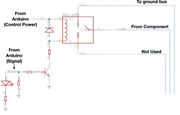
SeaBAT Plug Features... BAC Assembly... Membrane Inlet Exploded View Voltage converter schematic . . Relay shield example schamatic

18 19 21 24 25 28 34 35 39 40 42 42 46 47 51 54 59 60 63 64 67 D ive Locations . . . .

Methane seep distribution along the Cascadia Margin Subduction Zone Instrument Suite Integrated on ROV . . . . BDS Cruise Configuration . . . . D ive Site Im ages . . . .

4-1 ISMS Output Example . . . 70 4-2 Bubble Composition by Gas - All Samples . . . 73

(12)

4-3 4-4 4-5 4-6 4-7 4-8

Bubble Composition - All Samples . . . . .

Gas Fraction Distribution by Sample . . . . Bubble Composition by Site . . . . Bubble Composition - All Altitudes . . . . Bubble Composition - Half Meter Samples . Gas Fraction Distribution by Altitude . . .

77 81 83 85 87 90

B-1 Intercollection sample trends . . . 111

B-2 CH4 Fraction Distribution by Site . . . 116

B-3 N2 Fraction Distribution by Site . . . 118

B-4 CO2 Fraction Distribution by Site . . . 120

(13)

List of Tables

Oil Compensated Enclosure Material BDS Component Control Scheme Arduino Channel Control Scheme List of Arduino Commands . . . . .

3.1 Dive locations and depths...

Comparison . . 37

. . 51

. 52 . . . 5 6 . . . 6 6

Bubble Data - First Samples Only Statistics - All Samples . . . . Statistics - by Altitude . . . .

78 80 89 112 B.1 Bubble Data - All Samples . . . .

13 2.1 2.2 2.3 2.4 4.1 4.2 4.3

(14)

(15)

List of Algorithms

1 M ain Loop . . . 55 2 handleSerial() - Takes incoming serial data and performs an action . . . .103 3 waitTime () - runs a timer in the background . . . 104

(16)

(17)

Chapter 1 Introduction

1.1 Motivation

While carbon dioxide (C02) often receives widespread attention as the primary driver of

climate change, methane (CH4) also plays a critical role [1-4]. CH4 is over 30 times more

potent of a greenhouse gas and has a radiative efficiency 1000 W/m2-ppb greater than CO ₂[5].

While CO2 accounts for over 60% of atmospheric radiative forcing, its absolute atmospheric

concentrations are approximately 213 times that of CH4 [5]. According to the

Intergov-ernmental Panel on Climate Change (IPCC), greater than 50% of atmospheric CH4 comes

from anthropogenic sources, but natural sources such as wetlands and thawing permafrost account for a large portion as well [5]. Once CH4 is released to the atmosphere, its direct

radiative effect is powerful but short lived. A single molecule of CH4 has an average

life-time in the atmosphere of only 11y before it is oxidized to water vapor and then CO 2 [6].

Other natural sources of CH4 are large reservoirs stored as gas hydrate, a solid, ice-like

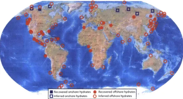
state, along the continental margins and in frozen tundra in the northern latitudes (Figure 1-1) [3,7]. Approximately 99% of the world's methane hydrate is stored in marine sediments and modern estimates place the total reservoir size at 1800 Gt C [1].

Methane clathrate hydrate (hereafter referred to as methane hydrate) is formed under high pressure, low temperature conditions by encaging CH4 molecules in a matrix of water

molecules [8]. In the ocean, the top of the hydrate stability zone (THSZ) begins in the water column usually around 300-500 meters below sea level (mbsl). Since temperature decreases and pressure continues to increase approaching the seafloor, the bottom of the hydrate stability zone (BHSZ) is located below the seafloor at the point where geothermal

(18)

Recoveredonshorehydrates 0Recovered offshore hydrates

OInferred onshore hydrates 0 Inferred offshore hydrates

Figure 1-1: Map displaying the worldwide distribution of known and inferred methane hydrates. Figure reprinted from [3].

temperature surpasses the effect of increasing lithostatic pressure and gas hydrates are no longer stable (Figure 1-2) [1]. The extent of this zone from the THSZ to the BHSZ is known as the gas hydrate stability zone (GHSZ). With some exceptions (see Section 1.3.2), CH4

within the GHSZ exists almost exclusively in its hydrate form, and when free gas escapes into the water column as bubbles, they form a hydrate film on the surface. Methane hydrates concentrate CH4 gas into a much smaller volume than free gas. One square meter of methane

hydrate contains over 170 n2 of CH4 gas, at standard temperature and pressure [1].

The existence of methane hydrates in marine sediment can often be inferred by acousti-cally imaged CH4 bubble flares originating within the GHSZ or by seismic sediment reflection

surveys [1]. The density of gas hydrate is typically less than that of the surrounding sed-iment so the change in the impedance of sound traveling through the sedsed-iment during a seismic survey results in a bottom simulating reflection (BSR) that is interpreted as the BHSZ [9,10]. The International Ocean Drilling Program (IODP) has recovered many sam-ples of gas hydrates sparsely distributed in the pore space of drill cores [11]. This finding has led to drastically reduced estimates of the world wide gas hydrate inventory which assumed that all of the available pore space in areas with BSRs were filled with hydrates [3].

With an atmospheric CH4 concentration of approximately 3 Gt C, the estimated global

inventory of methane hydrate has led to discussion of the potential climatological impacts

(19)

ocean surface 0 ocean water ternperatu 400 Sfegas + r dissolved

e

: 800 S' ga C 1200 _seafloor gas 0 1'600 I : as 0 10 20 30 Temperature (°C)

Figure 1-2: Schematic depicting the GHSZ. Hydrostatic pressure increases linearly with depth and the green line indicates water temperature. Inside the yellow zone, CH4 exists

in its gaseous state. Inside the purple zone, methane hydrates are stable. Once below the seafloor, the temperature increases until it it outside the GHSZ. Figure reprinted from [1].

if these reserves or a fraction thereof are rapidly released to the atmosphere due to warming

ocean waters (in the case of marine reserves) or warming atmosphere (in the case of the terrestrial reserves) [6, 9, 12-161. These discussions reference current rising temperature trends and historic thermal maximums shown in the paleoclimate record in which isotopically

light carbon tracers indicated elevated levels of atmospheric CH4 which could have caused

global scale warming [2,17,181.

There is a continuous release of CH4 gas bubbles from marine sediments in these methane

hydrate rich continental margins that may be amplified by rising ocean temperatures [1,6]. The ebullitive, or bubbling, CH4 flux from the seafloor, into the shallow mixed layer, and

ultimately into the atmosphere is poorly constrained. In order to understand the fate of the

released CH4 gas, it is important to know where the gas came from and how it is released

into the water column. The following sections explore our current knowledge of the sources of CH₄and methane hydrate in marine sediments (Section 1.2), the forcing mechanisms that cause its ebullition (Section 1.3), and a review of the studies that attempt to constrain its flux (Section 1.4).

(20)

1.2 Methane Sources in Marine Sediments

The origins of CH4 in marine sediments are divided into two categories: biogenic and

ther-mogenic [3,4]. Both biogenic and therther-mogenic production find their sources in organic material, but biogenic CH4 is created by biological processes whereas thermogenic CH4 is

created by geologic processes. Biogenic production takes place in the top layers of marine sediments over much shorter time scales (days) than thermogenic production [19]. Mean-while, thermogenic production occurs thousands of meters below the seafloor over periods of centuries [20].

The source of the gas can be determined by measuring the ratio of 13 to carbon-12 and comparing it to an internationally recognized reference material (Vienna Pee Dee Belemnite, VPDB). This comparison of ratios is expressed in delta notation (613C) and calculated by the following equation [21]:

613C(%) [(13= 12 measured- _{1 x 1000} _(1.1)

[(13C/12C)standard

-Methane gas from thermogenic sources tend to have a lower 613C (-20 to -50 %c) than that from biogenic sources (-58 to -90 %c). 613C between -50 to -58%o is a result of biogenic and thermogenic source mixing [19,22]. From these values, the predominant source of the CH4

can be determined.

1.2.1 Biogenic Sources

The primary source of biogenic CH4 in marine sediments is the remineralization of organic

carbon by anaerobic microbes [23]. The last step of this remineralization is performed by a unique set of archaea known as methanogens and can be simplified to the following reaction [2,4]:

C02 + 8H+ + 8e- -+ CH4 + 2H20 (1.2)

Organic carbon reduction in marine sediments is subject to a hierarchy of energetically favorable reactions. Valentine [4] describes this as the "redox ladder" in which a multitude of more thermodynamically favorable redox reactions occur before CO2 is reduced to produce

CH4. In general, the ladder begins with oxygen (02) and is followed by nitrate, Mn(IV),

(21)

is at the bottom of the ladder. Of all of these electron accepting species, the most abundant in marine sediment is SO42- whose preferential reduction results in a notable CH4 depletion

zone in the top layers (Figure 1-3). This zone can vary from a few hundred centimeters [19] to several hundreds of meters along the continental margins where methane hydrates are known to occur [3,25]. CH4 can be oxidized by SO42, so any CH4 that might be present is

consumed [19]. Once the sulfate is depleted, net CH4 generation can occur.

There is also a pathway for CH4 production even in the sediment layers where S042

-reduction is taking place. Fermentation of methyl amines and other organic sulphur com-pounds has been observed in sediment [4,19]. The reaction typically takes the form:

CH3- A + H2O - CH4+CO2 + A - H (1.3)

where A represents the amine. While the extent of these reactions in marine sediments is unclear, they have been observed in several freshwater environments and salt marshes [19].

Atmosphere Water colu Enclosed basin 0 ₀ tDiffusve -CH4,lux 0 1 2 Methane (pM) Sufate (m Methane (m Sediment C44+202 Aerobic( methanotrophy S CO2+ 2H20 M Methanogenes i --M) ~10 3hrmogenes Atmospheric flux Oilskin 3#Disotiuties HIydrate

:

Cold seeps Freegas Traditionalgasreservoirs

Figure 1-3: Summary of biogeochemical and transport processes affecting CH4. Figure

(22)

1.2.2 Thermogenic Sources

Thermogenic CH4 production begins with the deposition of organic material on the seafloor.

As more material is deposited, prior deposits are compressed, heated, and pushed further below the seafloor where it is broken into smaller molecules. In general, the hydrocarbons produced get smaller with increasing depth. The organic materials that serve as the precur-sors for deep hydrocarbon production are known as kerogens and range from low molecular weight (i.e., algae and plankton) to high molecular weight (i.e., land plants) [20,22]. Low molecular weight organic material is the precursor for type I kerogens while high molecular weight material forms type III kerogens [20]. At shallower depths (around 1500m), heavier crude oil production from type I kerogens dominates. CH4 production peaks much deeper

(around 2500-5000m) from mainly hydrogen-rich type III kerogens [201.

Types I and II kerogens can also lead to the production of CH4, but it is not as common

[19]. Once formed, hydrocarbons migrate up the lithostatic pressure gradient toward the seafloor. Lighter hydrocarbons such as CH4 are more likely to reach the surface due to their

greater buoyancy and ability to permeate sediments [20,26].

1.3 Free Methane Forcing

When the thermogenic CH4 nears the seafloor, it forms a reservoir of free gas below the

BHSZ where it may mix with any biogenic CH4 that is present and then migrates through

the overlying sediment where it is released as bubbles in the water column [20,27]. CH4

bubble seeps are erratic in their intensity and periodicity [28] with reported hourly [28,29], seasonal [29-31], and decadal [27] variability. The reasons for this ebuillitive variability are not well understood.

The basic mechanism by which gas is transported to the seafloor is by the formation of fractures in the sediment. Once the gas has reached the seafloor, its variability might be regulated by hydrostatic pressure. There are three predominant theories proposing how the transport from gas reservoirs to the seafloor occur and why the rate and occurrence might be variable: (1) seismic forcing (Section 1.3.1), (2) hydraulic forcing (Section 1.3.2), and (3) tidal forcing (Section 1.3.3). Seismic and hydraulic fracture theories outline possible transport mechanisms and seep periodicity while tidal forcing theory focuses on periodicity alone.

(23)

1.3.1 Seismic Forcing

The proposed mechanism for seismic forcing is rather simple - seismic activity places enough shear stress on the sediment to create fractures for gas to flow through [29]. Several studies have inferred earthquake driven CH4 ebullition using various modeling techniques or

observ-ing bubble activity after a quake. Work by Kessler et al. [32] used radiocarbon datobserv-ing and hindcast modeling to determine that an active CH4 seep in the Cariaco Basin off the

north-central coast of Venezuela began between 1958 and 1967. A moderate earthquake occurred in the Caribbean Sea 70 km northwest of the Cariaco Basin seep in 1967 that could have initiated the ebullition. In another study, Alpar [33] first noted a significant increase in bub-ble seep activity using ship-mounted multibeam sonar in the Gulf of Izmit, a small, isolated inlet off of the Sea of Mamara in northwest Turkey, after the large Kocaele Earquake in 1999. This increased seep activity has been confirmed and investigated further by several other studies [34-36]. Field and Jennings [37] presented evidence of seismic forced seep activity off the coast of northern California during an eight year survey of the Klamath River delta. In the middle of this survey (November 1980), an earthquake occured and the authors noted increased, short term (less than three years) gas ebullition using seismic reflection surveys and ship mounted side scan sonar. Finally, a study by Obzhirov et al. [38] using temporally sparse acoustic flare observations has indicated seismic activity may play an important role in bubble flare formation and periodicity in the Okhotsk Sea near Russia. These studies rely on multiple discrete observations or inference to establish the role of seismic activity in CH4 ebullition, but better temporal resolution is needed to constrain its effect.

Many studies with enough temporal resolution and range to attempt to demonstrate the correlation between gas ebullition periodicity and seismic activity measure dissolved CH4 concentration in pore fluid or acoustically image bubble flares. Elevated dissolved

CH4 concentration can result from methane-rich water flow from the sediments or from CH4

bubbles dissolving as they rise through the water column. Thus, dissolved CH4 concentration

is a good proxy for the presence of bubbles, but it is not definitive. Some studies have reported increased dissolved CH4 concentrations after earthquakes [32,39] while some could

not correlate observed periodicity with earthquakes at all [40, 41]; thus, using dissolved CH4 activity to show a correlation between seep and seismic activity is fairly inconclusive.

(24)

backscatter from the CH4 is directly observed. Only one study, performed by R6mer et

al. [29], has made continuous, long-term acoustic observations of a seep over a large temporal scale at Clayoquot Slope off the coast of Vancouver, Canada. Despite observing over 70 earthquakes during the year long study, no correlation could be found between bubble flare periodicity and seismic activity.

1.3.2 Hydraulic Fracture

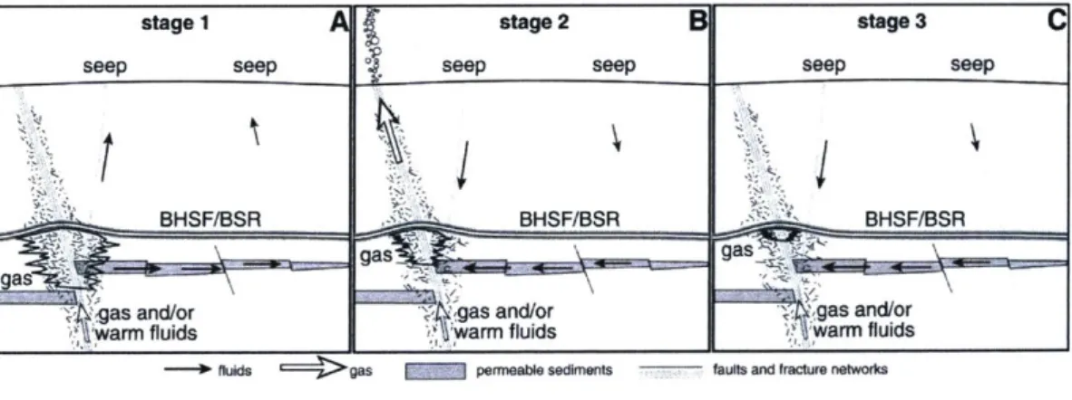
Tryon et al. [42] describe a three-stage mechanism by which a reservoir of gas can fracture the hydrate boundary above it and can migrate to the surface (Figure 1-4). In stage one, the gas reservoir volume increases as it is fed by porous sediment passages from deeper sources and displaces pore fluid into the water column (Figure 1-5) [10, 27]. This migration has been studied in detail by IODP cruises, seismic reflection surveys [10,11,27], and numerical simulation [43]. In stage two, the volume of accumulated gas is large enough to fracture the sediments above the reservoir which allows the gas to rapidly escape [42]. In the final stage, the gas volume has decreased to a point that pore fluids can begin to flow back into the reservoir area. Eventually gas flow will stop and the process can begin again. This is a dynamic process that takes decades to complete. Daigle et al. [43] modeled the temporal scale by considering a wide array of dynamic factors including reservoir size and depth below the seafloor, water depth, and overlying sediment type at Hydrate Ridge, an extensively studied site off the coast of Oregon known for frequent methane seepage. The authors estimated that the three stages of hydraulic fracture takes 52-61 years at this site.

stage 1 stage 2 stage 3 C

seep seep . seep seep seep seep

BHSF/BSR BHSF/BSR BHSF/BSR

gas gas

as

as and/or as and/or gasand/or

'warr fluids ;warr fluids warm fluids

fluids gs permeable sediments faults and fracture networs

Figure 1-4: Schematic drawing depicting the stages of hydraulic fracture at Hydrate Ridge along the Cascadia Margin. Figure reprinted from [42].

(25)

Figure 1-5: Illustration of the proposed migration path along porous sedimentary pathways at Hydrate Ridge. The migration pathway, "Horizon A," is identified as a second seismic reflection below the BSR [3,27]. Image reprinted from [27].

The propagation of free gas through the GHSZ is confounding in the hydraulic fracture model. Intuitively, the gas traveling through the GHSZ would quickly form into methane hydrate and block flow. However, studies have shown that the gas can slowly migrate through fractures by forming hydrate boundaries around the channels that will separate the gas from the surrounding pore water - a key requirement of hydrate formation [44,45]. Torres et al. [46] has altered the original fracture theory to include the fact that free gas can occur within the GHSZ. In this modified model, the possibility that the fracture can occur at a continuum of depths rather than just below the BSR is considered.

1.3.3 Tidal Forcing

Tidal forcing is the most widely observed cause of short-term methane bubble flare pe-riodicity [29]. As with seismic forcing, there are few studies with the required temporal resolution to link tides with flare periodicity. However, tides are predictable whereas earth-quakes are not. Several studies have noted a tidal component to the fluctuation in gas ebullition [29,46-50] based on short term studies of hours to days, while some studies fail to establish a link [51]. Boles et al. [471 and Rmer et al. [29] have quantified the relationship. Boles et al. noted tidal components to the gas flux from a seep at a depth of 65 m at Coal

Bubble 0 0

2000

plume

0

00.*

500 m

000' 4nt 00 ;

(26)

OZ-17-Point off the coast of California. The seep they studied was covered by a large metal "tent" that was already in place for collecting and pumping gas to a shore facility for industrial use. The researchers used the time dependent flow variability to the shore facility as a proxy for time dependent seep intensity. In the frequency spectrum of the fluctuations, the group noted strong peaks at 12 h, 12.4 h, 23.9 h, and 25.8 h corresponding to S2, M2, K1 and 01 tidal frequency constituents. In this study, the seep site was isolated from the change in hydrostatic pressure caused by the tidal cycle. Additionally, the ebullition could have been affected by the build up of gas at the top of the tent that may have created an artificially high pressure inside the tent after a vigorous release of bubbles.

R6mer et al. [29] used a node of the Ocean Network Canada's North-East Pacific Time Series Underwater Networked Experiments (NEPTUNE) array at Clayoquot Slope (1250 mbsl) to quantify tidal contributions to CH4 ebullition along the Cascadia Margin. The study collected approximately a year of continuous data from a rotating multibeam sonar that was co-located with a known bubble flare combined with a current meter and bottom pressure recorder. They found a 12.4h periodicity in the seep which corresponds to the M2 tidal frequeny constituent. Interestingly, only one tidal cycle appeared to contribute to the periodicity at the deeper Clayoquot Slope seep. This may have been due to the fact that the range in tidally influenced pressure changes, as measured by the bottom pressure recorder at Clayoquot Slope, was only 0.15% of the hydrostatic pressure at 1250m while the tidal pressure changes at Coal Point were 3.3% of the hydrostatic pressure at 65m.

Tidal forcing models hinge on changes in hydrostatic pressure (PH) with the rising and falling tides. Boles et al. [47] describe a pore activation model in which the change in hydrostatic pressure affects pore sizes differently. R6mer et al. [29] reference a conduit dilation model in which the change in hydrostatic pressure, in tandem with changes in shear stress in the sediments, can form a pathway for gas release. These two models are explored in more detail below.

Pore Activation Model

In the bubble forcing model proposed in the Coal Point study, bubbles originate in a reservoir and travel in slugs to the surface after release through sediment pores into a fracture channel.

(27)

In this model, bubbles will be released if the following is true:

PH < PST + PF (1.4)

where PH is hydrostatic pressure, PST is the Laplace pressure of the bubble, and PF is the fracture pressure [47]. Due to the viscous interaction between the gas and the surrounding sediment in the fracture, PF decreases as the gas moves further from the source. PST is dependent on the surface tension (T) of a bubble and the bubbles radius (r) [47]:

PST = Pinside - Poutside = (1.5)

rbubble

As a bubble forms in a pore, PST and PF increase until they reach the point at which the bubble is released into the fracture. When a bubble is released, PST + PF momentarily

drops and the pore becomes inactive [3,42,47].

Conduit Dilation Model

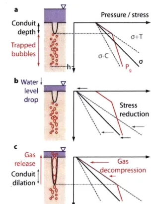
The conduit dilation model proposes a dynamic physical change in the sediment rather than the bubbles as a mechanism for release (Figure 1-6). In the model, there is a conduit near

the surface (formed as described in Section 1.3.1 or 1.3.2) from which the bubbles might be released based on the effective stress (') felt by the sediment:

o' = - Pg (1.6)

where Pg is the gas pressure in the sediment and o is real stress. Pg is a function of PH alone, while a is a function of both PH and lithostatic pressure [52]. As PH decreases, the volume of the gas increases and the cavity in which the gas is held deforms. Conduit dilation occurs

when o' becomes negative and reaches the tensile limit of the sediment. The conduit dilation and cavity deformation work in tandem to release gas. If hydrostatic pressure increases to the compression limit (C), the conduit can plastically close [52].

1.3.4 Composite Mechanism

The three forcing mechanisms (seismic, hydraulic, and tidal) cannot individually characterize all CH₄ seep behavior. Most studies observe changes in flow that cannot be fully accounted

(28)

a

Pressure stress Conduit

depth

.-... .

o+T Trapped 'N bubbles c _C

h

P

b water level drop Stress

*

reduction

C Gas release Gas . Conduit : decompression dilation ....

---Figure 1-6: Depiction of the effect of water level drop on the conduit system. a) In the initial condition, the water level (shown in purple) is high and there are trapped bubbles below the conduit. The depth at which the conduit opens is when o' reaches its tensile limit, -T. b) When water level drops, the stress on the system (mainly in the form of hydrostatic pressure) drops. For the purpose of this drawing, the gas pressure remains the same. c) In the final step of the model, the gas decompresses and the conduit opens at the depth dependent tensile limit. T(h) increases linearly with depth in the sediment. Since the sediment stress is lower due to decreased hydrostatic pressure, or' reaches its tensile limit deeper in the sediment. Thus, the conduit opening expands and allows gas to escape. Figure reprinted from [52].

for by tidal variation [27,40,46,53]. Studies that try to constrain flow based on hydraulic or seismic fracture lack compelling data to definitively say that flare periodicity is due to either mechanism alone. However, if all three mechanisms are viewed in tandem, a more complete view of the erratic ebullition can be achieved.

The hydrate-coated gas transport fractures will not always be free flowing. The pathways can become capped by hydrate if the flow ebbs to the point where vertical water intrusion is allowed [11]. Indeed, evidence of these caps is readily seen in seismic imaging [27,29] and by core samples showing bubble-textured hydrate deposits [10, 44-46]. Hydrate cap formation is dependent on reservoir gas pressure and thus will be highly unpredictable.

(29)

The caps would need to be fractured by hydraulic or seismic means in order for flow to continue. Additionally, reservoir gas pressure can have a great effect on a seep's sensitivity to hydrostatic pressure [10]. In a situation where the gas pressure is much greater than the hydrostatic pressure, flow will be vigorous and not susceptible to pressure changes. As the reservoir pressure approaches PH, the seep will be more susceptible to the effects of changing PH, and the seep will be more likely to form a hydrate cap that must then be hydraulically fractured.

1.4 Ebullitive Methane Flux in Marine Environments

The amount of CH4 released from marine sediments that reaches the air-sea interface is

poorly constrained. In shallow (< 200 m) or very vigorous bubble flares, a clear CH4 flux

at the air-sea interface can be observed [39,54,55]. However, it is often assumed that CH4

from flares originating deeper than approximately 500m does not make it to the ocean surface [1, 56, 571. Since the early 2000's, there has been a significant effort attempting to constrain this problem [1,39,51,55,58-621.

The most common methods for determining bubble flare rise in the water column are acoustic imaging [26,53,56,58,60,62-64], modeling [55,65], and using optical instruments [59, 61, 66-68]. The purpose of these studies was to quantify the extent to which CH4 is

transported from the seafloor to the water column. In studies where acoustic imaging was used extensively, multibeam sonar was used to visualize how high in the water column the bubbles rise. This method was used to successfully determine that the bubbles do not often make it to the surface of the water. However, the sonar can have difficulty imaging the terminal stage of the bubble rise because the bubbles are much smaller and the sonar is tuned to image bubbles in the bulk of the flare.

Optical instruments track the rate of change of a bubble's radius once it is emitted from the seafloor. This method requires a remotely operated vehicle (ROV) to follow the bubble through the water column and to track how quickly the bubble shrinks or to remain stationary and observe the bubble flare at its source. Except in the most vigorous flares, it is difficult to find bubbles in the water column once above 10-20m above the seafloor. In order to track the bubbles, Rehder et al. [59] surrounded the bubbles with a clear plastic box and followed them through the water column. This method was problematic because

(30)

the bubbles in the box are not experiencing thedynamic geochemical gradients and currents that a bubble normally would during its ascent, thus affecting the rate of bubble dissolution. Additionally, the rise rate of the bubble is biased upward due to the drag forces imposed by the box. The stationary optical methods rely on data from a single altitude and must extrapolate the rate of change of the bubble radius [61,66-68]. In a bubble's rise, it may encounter a wide range of ambient conditions that may cause it to shrink at a rate different than at its source.

Both the acoustic imaging and optical instruments fail to consider the chemical compo-sition of the bubble after it leaves the seafloor. The dissolved gas concentration in the water surrounding the bubbles is below saturation with respect to CH4 so this extreme

concen-tration gradient causes the CH4 inside the bubble to diffuse into the water column. Gases

already dissolved in the water column such as 02, C0₂, and nitrogen (N2) diffuse into the

bubble and replace some of the volume that is lost [21,65]. The gas exchange has been modeled in a few studies [55,65], but little work has been done to validate the models in the field. Leonte et al. [21] used the Texas A&M Oil spill (Outfall) Calculator (TAMOC) [69,70] to quantify the fraction of hydrocarbon gas remaining in a bubble released from a 890m deep seep at different rise heights in the Gulf of Mexico. The authors used the natural stable carbon isotope fractionation that occurs when CH4 dissolves from a bubble to determine

the fraction of CH4 that dissolved from a bubble flare into the surrounding water column at

multiple depths and compared it to the remaining fraction of CH4 predicted by TAMOC.

The study found that within the first meter of bubble rise, 58.2±31.1% of the CH₄had left the bubble and that 97.5±4.7% of the CH4 had left the bubble after 766 m of bubble rise

(124 mbsl).

Another method to constrain ebullitive CH4 flux is to consider the chemical composition

of a bubble once it has left the seafloor. Chemical composition analyses are not often performed because it is difficult to collect gas samples from the flare and analyze them. To date, few authors have performed chemical composition analysis on bubbles collected from a CH4 flare. Leonte et al. [21] collected bubbles from a seep in the Gulf of Mexico with

modified Niskin bottles attached to a ROV and brought them to the surface for separation by gas chromatography and compositional analysis by thermal conductivity and a flame ionization detector (FID). The collection apparatus allowed the bubbles to expand as the ROV returned to the surface and the compositional analyses were performed in a ship-board

(31)

laboratory. Baumberger et al. [71] collected bubble samples from the Cascadia Margin in the northeast Pacific in a custom gas-tight bottle connected to a ROV that did not allow the bubbles to expand as they were brought back to the surface. The authors analyzed the samples in a similar manner to Leonte et al. except the analyses were performed at a shore-based facility after the cruise.

These two studies were limited by their collection methods and ex situ chemical analyses. Both collection methods allowed for a limited number of samples to be collected on each dive. Leonte et al. were limited in the number of samples they could collect on each dive and only collected three samples in the entire study. Baumberger et al. dove with multiple gas-tight bottles that could only be used once per study since the chemical analyses were performed on shore. Additionally, the authors were limited by the number of collection bottles that could be brought on the dive and the cruise. As a result, the study only analyzed five samples. With all of the sample analyses occurring ex situ in both studies, the authors had no ability to employ dynamic sampling strategies based on real-time results from prior samples. Finally, the sparse sampling patterns that had to be employed because of resource-heavy sampling methods gave spatiotemporally limited results.

In order to improve the spatiotemporal range and resolution of bubble chemical compo-sition studies, a sampling tool that can be used multiple times in a single dive is needed. If the samples are analyzed in situ and the operator has access to the real-time output from an in situ instrument, a dynamic sampling plan can be used to better characterize a CH4

seep. This multi-use sampling tool with in situ analysis techniques will be limited by ROV dive time rather than the number of sample bottles. Michel et al. [72] successfully collected CO2 bubbles and analyzed them with an in situ laser spectrometer that is used to measure

carbon isotopes of CH4, but this did not allow for the full characterization of a bubble's

chemical composition.

An in situ mass spectrometer (ISMS) (e.g., Wankel et al. [73]) would be a more useful tool to characterize a bubble's chemical composition. The ISMS is a type of membrane inlet mass spectrometer (MIMS) in which a thin, semi-permeable membrane is used to allow dissolved gas from a sample stream to diffuse into the mass spectrometer for analysis. The ionization chamber and detector of the mass spectrometer are kept at an extremely high vacuum (10-5 Torr) thus the pressure gradient accross the membrane is immense. The instrument is built around a Stanford Research Systems Residual Gas Analyzer (SRS RGA100) in which

(32)

the ion signal of discrete ion mass charge ratios are plotted against time. SRS has developed proprietary software that provides a real-time display of the time course response of the instrument.

The goal of this thesis is to outline the development of a bubble delivery system (BDS) for collecting bubbles for analysis by the ISMS developed by Wankel et al. [73]. Chapter 2 outlines the design and development of the BDS. Chapter 3 describes first deployment of the BDS. The chemical composition results from the deployment are discussed in Chapter 4 and concluding remarks are presented in Chapter 5.

(33)

Chapter 2 Bubble Delivery System Design

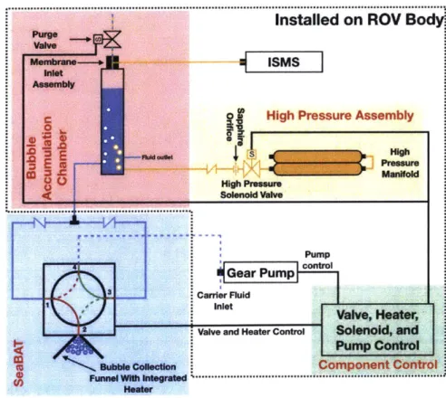
The Bubble Delivery System (BDS) is designed to be manipulated by an ROV to sample and analyze bubbles in situ at depths of up to 1200 m. The construction of the BDS can be broken down into four major subsystems: (1) the deep-sea. Bubble Acquisition Tool (SeaBAT), (2) the bubble accumulation chamber (BAC), (3) the high-pressure purge assembly (HPA), and (4) the component control circuitry. These four subsystems work in tandem to collect small aliquots of bubbles and deliver them to an in situ mass spectrometer for analysis (Figure 2-1). This chapter will begin with a brief overview of the operation of the BDS (Section 2.1), followed by general design decisions (Section 2.2), and finally by a detailed discussion of each of the subsystems (Sections 2.3 - 2.6).

2.1 BDS Overview

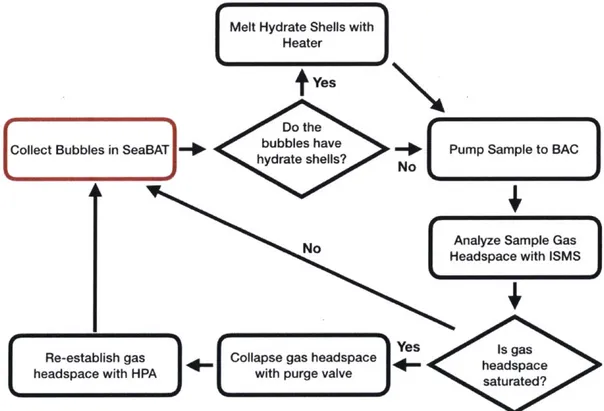
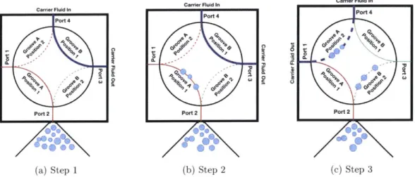
The first step of the bubble sampling workflow (Figure 2-2) is accomplished by the SeaBAT. The SeaBAT is deployed by the ROV manipulator arm to collect bubbles for analysis and is built around a low pressure, four port, two position stream selector valve (C45R-8144; Valco Instruments Company Incorporated, Houston, TX). Bubbles are collected in a funnel that is attached to the exterior of the valve enclosure and enter the head of the valve via passive buoyant forces. If operating in the GHSZ, the bubbles may have a hydrate shell that must be melted before rising into the valve head by a heater that is integrated in the SeaBAT. To collect a bubble sample, the valve is cycled and the bubble is placed inline with the discharge of a variable speed, bi-directional gear pump (McLane Research Laboratories, East Falmouth, MA) whose suction source is ambient seawater. Design specifics and sampling

(34)

Installed on ROV Body

Purge Valve Membrane- S Inlet Assembly

High Pressure Assembly

0 High Pressure Solenoid Valve Pump control Gear Pump 4 3- Carrier Fluid t Inlet Valve, Heater,,

Valve and Heater Control S lOd, and Pump Control M

~

Bubble Collection ::Component Control

Funnel Wi Integra..

Heater

Figure 2-1: Overview of the BDS shown coupled to the ISMS. Blue lines indicate fluid flow paths, yellow lines indicate gas flow paths, and black lines indicate electrical connections. Individual BDS components are labeled in red. In the SeaBAT, red lines indicate Groove A and green lines indicate Groove B. Solid lines indicate groove connections in Position 1 and dashed lines indicate Position 2.

flow paths of the SeaBAT are detailed in Section 2.3.

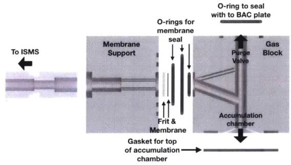
After a bubble sample has been collected by the SeaBAT, the gear pump is used to transfer the sample to the BAC at 125mL/min. The BAC consists of a collection chamber, membrane inlet assembly, purge valve, and ISMS. The membrane inlet assembly sits on top of the main chamber. A volume of air (gas headspace) is established in the interior of the membrane inlet assembly and the top portion of the main chamber while the bottom portion of the main chamber is filled with water. The sample will enter the BAC via a port at the bottom of the main chamber, rise to the top, and burst in the gas headspace. The resulting change in composition of the gas headspace is determined by the ISMS which will provide real-time results.

(35)

should be collapsed (i.e. filled with water) and then re-established with air from the HPA and the purge valve from the BAC. To collapse the gas headspace, the purge valve is opened and the gas headspace will empty to the surrounding water. When the gas headspace is fully collapsed, the purge valve is shut. To refill the gas headspace, the high pressure solenoid is opened and high pressure air flows from the high pressure manifold, through the high pressure solenoid and flow control components into the BAC where it collects at the top of the main chamber. Details of the design and operation of the BAC and HPA are in Sections 2.4 and 2.5, respectively. Electronic control of these components is detailed in Section 2.6.

Melt Hydrate Shells with

Heater I

Yes Do the

bubbles have

~

[Collect Bubbles in SeaBAT -t _{< hydrte shlls?}shels? No

No

Re-establish gas headspace with H

Analyze Sample Gas Headspace with ISMS

Collapse gas headspace Yes hsagas

PA _{with purge valve} _seadae?

Figure 2-2: BDS sampling workflow. The red box indicates the beginning of the workflow.

2.2 General Design Considerations

Deploying the BDS in the deep ocean presents a unique set of design challenges. The mate-rials used must be able to perform as desired in cold temperatures (0-4°C), high pressures (>100 bar), and corrosive salt-water environments. Since this instrument is deployed by an

Pupa C

PumpSapet A

(36)

ROV, the components cannot be too heavy or large. Additionally, any component, such as the SeaBAT, used by the ROV manipulator arm is subject to unexpected mechanical shock and cable strain due to the dynamic nature of the arm movement. To this end, several general material selection and design considerations have been applied to the BDS design.

2.2.1 Oil Compensated Enclosures and Structural Materials

Electronic components such as valves and circuit boards cannot be exposed to sea water. Since the BDS is deployed in situ in the deep ocean, the only options to protect these components from exposure to sea water is to enclose them in a pressure vessel or to oil compensate them. Pressure vessels keep electronics completely dry and under atmospheric pressure. This is ideal for sensitive electronics that cannot withstand the intense pressures of the deep ocean (e.g., circuit cards and microcontrollers). Pressure vessels that can withstand the pressures outlined above are often made of stainless steel or titanium. Both of these materials are heavy and expensive to machine.

A lower cost option is to oil compensate the electronics. This method protects electronics by enclosing them in a housing that is filled with mineral oil. Mineral oil is effectively incompressible, so the differential pressure across the walls of the enclosure will be minimal. Thus, lighter components (often plastic) can be used for the enclosure walls. The drawback is that the electronics that are oil compensated are exposed to hydrostatic pressure. This limits the application to components that can withstand high pressure such as motors, valves, and junction boxes. While the BDS employs some electronics that cannot be oil compensated (see Section 2.6), there are several components that can withstand high pressures and thus were oil compensated:

1. SeaBAT Valve 2. BAC Purge Valve

3. HPA High Pressure Valve

The general design of an oil compensated housing is the same regardless of what is en-closed. The two features that are common to all oil compensated housings are the enclosure itself and a flexible bladder. For the BDS, several types of plastic commonly used for these type of enclosures were considered: Acetyl copolymer, Acetyl homopolymer,

(37)

polyvinylchlo-Table 2.1: Comparison of oil compensated enclosure material choices. Acetyl homopolymer was chosen because of its high strength, ease of machining, and lack of porosity.

Material Temperature Range Tensile Strength Ease of Cost

(-C) (kPa) Machining

Acetyl Copolymer -29- 82 44,126 Easy $$

Acetyl Homopolymer -29- 82 62,052 Easy $$$

Polyvinylchloride (PVC) -17- 82 4,136 Moderate $

High Density Polyethylene 10- 82 27,579 Moderate $$$

Nylon -40- 85 77,221 Difficult $

ride (PVC), high density polyethylene (HDPE), and nylon. The important material charac-teristics are outlined in Table 2.1. All of the oil compensated enclosures were machined and built by the author in DunkWorks,1 so the difficulty of machining was an important factor in the material choice. For that reason, Nylon was not used. Additionally, PVC becomes brittle at low temperatures and HDPE did not meet the minimum temperature requirement so neither was a good choice for this application. Although acetyl homopolymer has a higher tensile strength than acetyl copolymer, it is slightly more expensive. More importantly, the manufacturing process of large acetyl homopolymer stock often introduces low density air pockets that can affect the structural integrity of the component. For those reasons, acetyl copolymer was chosen for this application.

Although considered mostly incompressible, under large pressure increases, the volume of a fixed mass of oil decreases. The extent of the compression is given by [74]:

-AV

AP-(2.1)

Vo Koji

where AV is the change in volume, Vo is the starting volume, AP is the change in pressure, and K01 is the bulk modulus of the oil. Given a maximum expected pressure change of

100 bar and Koil is 2.41 GPa [74], the volume of the oil will only compress by 0.4 %. The oil is allowed to compress by the use of flexible silicone bladders and all of the enclo-sures employed two such bladders. The first consisted of a 1.6 mm silicone sheet compressed by a 9.5 mm piece of acrylic plastic. The acrylic had a 038 mm hole cut in the center to allow the bladder to experience the hydrostatic pressure, flex inward, and compress the oil. This single bladder was expected to accommodate the oil compression, but a fill line was

'DunkWorks is a rapid prototyping facility and is a part of the Center for Marine Robotics at Woods Hole Oceanographic Institution, Woods Hole, Massachusetts

(38)

needed to add and drain oil from the enclosure. The volume of this 06.4mm i.d. fill line was used as a backup bladder to accommodate at least 90% of the expected compression as a safety margin to avoid crushing the enclosure. This is an overly cautious inclusion because the internal volume of each of the enclosures was calculated as if there was no component in the enclosure. For example, the BAC Purge Valve enclosure internal volume was calculated

without taking into account the volume that the valve itself would occupy.

The tubing also served as the oil fill line, so the caution came with little cost. At one end of the tubing, a quick-connect tubing connector was included so the enclosure could be filled from an external tank. A vent to allow the air displaced by the oil was located opposite of the oil fill line and is sealed with a gasketed screw when not in use. To fill the enclosure, the vent screw is removed and oil is added through the fill line. When oil begins to seep from the vent hole, the sealing screw is replaced and any excess air bubbles are evacuated using the fill line.

Details of the fill line internal volume and other features of the oil compensated enclosures are included in Sections 2.3, 2.4.3, and 2.5.2.

2.2.2 Metal Components

Salt water can cause corrosion that can bind fasteners and dissolve metal components. Gal-vanic corrosion can be a concern in strong electrolytic environments such as sea water, as well. To counteract these two effects, 316 Stainless Steel was chosen for all metal compo-nents (e.g., solenoid valve casings, high pressure tubing, fittings, fasteners, etc.) with few exceptions that will be discussed in the component descriptions.

2.2.3 Tubing and Electrical Connectors

With the exception of the HPA, the pressure inside all of the components and tubing is the same as hydrostatic pressure. Swagelok® 316 Stainless Steel tube fittings and adaptors (Swagelok Company, Solon, OH) were used throughout the instrument. In order for these fittings to create a good seal, the fluid tubing must be hard but must also be flexible because it will run along the ROV manipulator arm from the SeaBAT to the ROV body. The tubing must be transparent in order to observe bubbles moving through it. For these reasons, flexible nylon tubing was chosen for all fluid tubing. In all high pressure applications, 1/4 in.-316 stainless steel tubing rated to 4,300 psi was used.

(39)

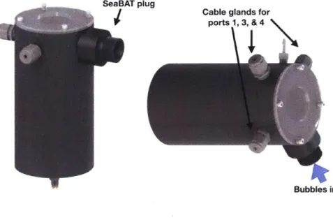
SeaBAT plug

Cable glands for ports 1, 3, & 4

Bubbles in

Figure 2-3: Rendering of the SeaBAT assembly.

All electrical connectors that are exposed to water are SubConn Micro Circular (Mac-Cartney Inc., Esbjerg V, Denmark). Bulkhead connectors are male and all inline connectors are female. Molex inline connectors (SL 70066 Series) are use for all hook-ups inside pressure

vessels and oil compensated enclosures.

2.3 SeaBAT Design

The SeaBAT consists of three major components: the (1) selector valve, (2) funnel plug, and (3) heater. The valve is oil compensated as described in Section 2.2.1 in a cylindrical

enclosure with exterior dimensions of approximately 011.4cm x22.8cm and an interior volume of 962 mL (Figure 2-3). From Equation 2.1, the oil will compress by 3.8 mL. Thus,

the oil fill line was 11 cm with an internal volume of 3.4 mL to accommodate 90 % of the oil compression. The SeaBAT was designed to meet the following requirements:

1. In order to reduce system complexity, a separate pump to move the bubble samples from the funnel into the valve is not used. Thus, the bubbles must be able to rise

(40)

passively into the valve.

2. The portions of the SeaBAT that come in contact with the sample must be chemically inert to prevent any chemical interaction with the gas.

3. Bubble streams are found at a variety of depths inside and outside of the GHSZ. The SeaBAT must be capable of sampling bubbles with and without hydrate shells.

4. The SeaBAT will be positioned above bubble streams by the ROV manipulator arm and its tubing/cable must be capable of extending the entire length of the arm.

2.3.1 Valve

(b)

Figure2-4: SeaBAT valve head images. a) Assembled valve head. Each port allows fluid/gas to enter or exit the valve head. b) Disassembled valve head. Streams that enter the assembled valve ports in the stator are connected via grooves cut in the rotor. To change the stream alignment, the stator rotates and the grooves will line up with the outlets of the ports in the stator. In this figure, the solid lines indicate the ports aligned by the grooves in position 1 while the dashed lines indicate the alignment in position 2.