HAL Id: hal-00372153
https://hal.archives-ouvertes.fr/hal-00372153
Submitted on 31 Mar 2009
HAL is a multi-disciplinary open access
archive for the deposit and dissemination of
sci-entific research documents, whether they are
pub-lished or not. The documents may come from
teaching and research institutions in France or
abroad, or from public or private research centers.
L’archive ouverte pluridisciplinaire HAL, est
destinée au dépôt et à la diffusion de documents
scientifiques de niveau recherche, publiés ou non,
émanant des établissements d’enseignement et de
recherche français ou étrangers, des laboratoires
publics ou privés.
Comparison of three algorithms for solving the
convergent demand responsive transportation problem
Rémy Chevrier, Philippe Canalda, Pascal Chatonnay, Didier Josselin
To cite this version:
Rémy Chevrier, Philippe Canalda, Pascal Chatonnay, Didier Josselin. Comparison of three algorithms
for solving the convergent demand responsive transportation problem. Intelligent Transport Systems
Conference, 2006, Toronto, Canada. pp.1096-1101. �hal-00372153�
Comparison of three Algorithms for solving the Convergent Demand
Responsive Transportation Problem
R´emy Chevrier, Philippe Canalda, Pascal Chatonnay and Didier Josselin
Abstract— Led by computer science and geography labo-ratories, this paper presents three algorithms for solving the Convergent Demand Responsive Transport Problem (CDRTP). Two of them are exact: the first one is based on a dynamic programming algorithm to enumerate exhaustively the sprawl-ing spannsprawl-ing trees and the second one is based on a depth first search algorithm. The third one is stochastic and uses a steady state genetic algorithm. These approaches address the problems of scalability and flexibility, are compared and discussed.
I. INTRODUCTION
The research deals with Demand Responsive Transport (DRT). In USA DRT is defined by the Federal Transit Administration and the Transit Cooperative Research Pro-gram (TCRP [22]) as ’Passenger cars, vans or small buses
operating in response to calls (...) to pick up the passengers and transport them to their destinations. A demand response operation is characterized by: (a) The vehicles do not operate over a fixed route or on a fixed schedule except, perhaps, on a temporary basis to satisfy a special need; and (b) typically, the vehicle may be dispatched to pick up several passengers at different pick-up points before taking them to their respective destinations and may even be interrupted en route to these destinations to pick up other passengers’.
In Europe, the definition is a little different and broader:
’DRT is an intermediate form of transport, somewhere be-tween bus and taxi wich covers a wide range of transport ser-vices ranging from less formal community transport through to area-wide service networks’ (Ambrosino et al. [1]) There
exist indeed many spatial organizations of the DRT services. We propose in this paper to tackle the specific Convergent Demand Responsive Transportation Problem (CDRTP). This is a relevant issue in the sense that numerous mobilities and individual destinations correspond to recurrent particular sites and places of interest: airports, centres of towns...
In France, this kind of DRT involves many urban and suburban territories. The actual purpose is to provide more efficient transport systems to save service expenses, traveled distances and pollutant emission. DRT may respond to these aims, due to its capacity to adapt to the demand. CDRT is indeed often provided to serve clients during the edge times hours (very early or very late in the day), on areas missing transportation services to complete the regular supply. It
R. Chevrier and D. Josselin are with Universit´e d’Avignon et des Pays du Vaucluse, UMR ESPACE (CNRS 6012), 74 rue Louis Pasteur, 84000
Avi-gnon France{Remy.Chevrier,Didier.Josselin}@univ-avignon.fr
P. Canalda and P. Chatonnay are with Laboratoire d’Informatique de l’Universit´e de Franche-Comt´e, LIFC (FRE CNRS 2661) NU-MERICA, Cours Louis Leprince-Ringuet, 25200 Montb´eliard France
{Philippe.Canalda,Pascal.Chatonnay}@univ-fcomte.fr
also can be connected to the core of the network through intermodal nodes to group the flows and therefore increase the global transportation service efficiency.
In our case, users have to book their seats at least 4 hours before the vehicles departure. This allows to process an asynchronous optimization (cars and drivers allocation, paths design) every day. Neither the sequence of the stops and the time schedule nor the shape of the routes are previously known. That is why this service can be considered as a DRT. A fruitful partnership between a Transport Authority (Communaut´e d’Agglom´eration du Pays de Montb´eliard, 140000 inhabitants), a private carrier (Compagnie des Trans-ports de Montb´eliard) and researchers from laboratories in Geography and Computer Science, joined in the TADvance group, provided the design of this convergent DRT whose concrete implementation is foreseen next year.
To be the less expensive possible and to respond to the users demand, a CDRT system has to consider fit-to-use and rigorously built data. In our study, we handle different geographical data: a finite set of stops where the clients can be picked up, a set of clients (transport requests) assigned to the stops, a topological network modeled using a graph with valued edges and finally one (or several) point(s) to converge, for only deliveries. Other constraints of service quality must be considered: the maximal duration of the route, the maximal delay at any pick-up point and the margin of time required at the convergence point (i.e. to get the following departure if needed).
The optimization consists in finding each day the minimal number of vehicles used, travelled kilometers, and occupa-tion rate of the vehicles. This leads to an interesting property of grouping passengers in the same vehicules and induces some social impacts due to the quality of such transport service. Indeed, the number of passengers remaining rather low, DRT facilitates a new kind of mobilities and relationship (reasonible size of vehicles, flexibility, comfort).
In this paper, we endeavour to show the relevance of different methods for solving the Convergent DRT Problem joining a reliable fitness and an acceptable efficiency of the method used. The CDRTP is specific in the way the destination point is fixed, allowing to keep under control the complexity in a certain room.
Such a problem has in fact multiple aspects. Given that the solving complexity grows exponentially according to the graph density, we propose three algorithms, each of them adapted to a complexity range. We do not present here neither the previous stage for designing the service according to user needs, nor the final step concerning users management Proceedings of the IEEE ITSC 2006
2006 IEEE Intelligent Transportation Systems Conference Toronto, Canada, September 17-20, 2006
(information delivery and booking) and service operating (ef-fective implementation of the paths and associated vehicles). We rather focus on two methodological aspects. Theoretical aspects of our research are not presented in this paper neither. We first present an outline of major related works to CDRTP, by focusing on exact or approximate solving meth-ods, describing and assessing the criteria and the targeted objectives. Thereafter we explain the methodology used and detail/compare three algorithms solving the combina-tive problem (two exact and a genetic one), all based on common data-processing objects: Convergence Graphs (CG) and Sprawling Spanning Trees (SST ). We end on a few experimental results and conclude on further works.
II. RELATED WORK
The CDRT problem is a parent to the np-complete TSP, for which various solutions exist. In its simplest configuration the CDRT problem is also linked to the Vehicle Routing Problem with Time Windows (VRPTW) [19]. In these two problems, the vehicles capacity can be taken into account, but also time windows in specific pick-up points on the territory. However, it is necessary to consider the delivery points with associated constraints. Finally, in a more complex DRT configuration, the problem can be associated to the Dial A Ride Problem (DARP). We shall be then interested in a generalization of the TSP, which corresponds more to the actual DRT, carrying clients to the destination point linked to the regular transport network. A generalization of this problem is the N-TSP, that we solved with N vehicles by partitioning, or spanning a territory into N smaller territories. The exact methods are not used because of their unsuffi-cient robustness. Indeed the major drawback remains the scalability. Thus approximated methods are preferred, like approximation schemes [21].
Another variant of the generalized TSP is the Pickup & Delivery TSP ([20], [5]), where goods and passengers are picked up and dropped off to precise destinations. For that problem various forms also exist, for which different approaches are proposed [17] to solve this problem: the k-PDP. Other TSP forms combine the N-TSP to thek-PDP, for example the k-PD N-TSP [14], which generalizes the TSP and takes into account the capacityk of one vehicle.
Unfortunately these approaches do not take into account neither the number N of vehicles, nor any QoS. Indeed, a more general solution of the DRT problem requires to consider the human and material resources [16]. Software so-lutions exist, that must better respond to constraints imposed by the users requests, and include the available resources. Some proposals consider hazards (is a vehicle broken down?) and adapt routes in consequence.
The genetic approaches are preferred to Branch & Bound approaches when we address the problem of the scalabil-ity or when the knowledge of a problem and its solving are unsatisfactory. With these approaches, multi-objective evaluation functions could be considered. They apply strate-gies for solving np-difficult problems [12], especially those
in relation to transportation. Some works propose a real-time approach for optimizing vehicles networks ([9],[13]). Crossover and mutation operators reduce the number of used vehicles, without penalizing clients or increasing travel times. About spanning trees, various approaches exist. We can cite the works of Raidl and Julstrom ([2],[11],[3]), who use evolutionary algorithms to encode spanning trees in undirected graph problems.
Our contribution follows previous works [7], that describes a CDRT system using the∞-PD TSP with n pick-up points ≥ m deliveries = 1 and solving simultaneously the N-TSP. The actual operational systems suffer from a lack of robustness (scalability) and flexibility. Indeed, they fail in proposing a simultaneous convergence to several points, by solving the∞-PD TSP with n ≥ m ≥ 1 for a single vehicle and always by solving simultaneously the N-TSP.
III. EXACT AND APPROXIMATE SOLVING METHODS
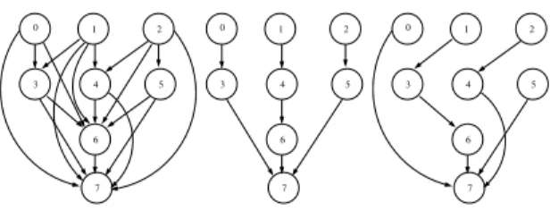
We propose three solutions for solving the CDRTP. The first ones are exact and the third one is stochastic. The first exact approach is based on a dynamic programming algorithm to enumerate the exhaustive set of solutions. The second one is based on a depth first search algorithm to enumerate the exhaustive set of optimal solutions. The last one is stochastic and based on a genetic algorithm, that allows the evolution of a population of solutions to the optimal solutions set. Our algorithms handle input matrices and adjacencies lists as well. These three methods lay on a common data modelling. According to a set of demands matched to a transport network including stops, we are able to build a Convergent Graph (CG) from all the requests to the convergent point (cf. example figure 1). The CG is directed, acyclic and transitive and enhances a total order of nodes. From this CG, we generate a large set of Sprawling Spanning Trees (SST) that supports the underlying logical structure of the generic CDRT problem. From a one-pass run on the graph, we can demonstrate that all valid solutions are computable and take the form of SST (cf. [18]). CGs and SSTs construction and properties has already been described in a recent publication ([6]). 3 4 5 6 2 1 7 0 3 4 5 6 2 1 7 0 3 4 5 6 2 1 7 0
Fig. 1. Convergence graph with 8 vertices and two of its SST
A. Dynamic programming algorithm
We present now the functioning of the dynamic program-ming algorithm (DPA) solving the convergent N-TSP, with a case study and improvements obtained on various mono-convergent transitive graphs.
1) Description: The proposed DPA is based on a classical
sequential iterative algorithm. First, we obtain the minimal nodes of the graph (i.e. nodes having no predecessor), and also the convergent nodes (i.e. nodes having no successor). From minimal nodes we create the first sprawling spanning tree (SST), which is composed of as many partial sprawling spanning trees (PSST) as many minimal nodes in the graph. So, at this step, we build a PSST made up with a minimal node and we add this PSST to the first SST.
The second part of the algorithm manages all the edges of the graph. For each node, neither minimal nor convergent (the destination point), we compute the list of edges, incident to node n. For example, on the figure 1 node 4 has two incident edges : (1, 4) and (2, 4). With the list ledges of incident edges to noden, we can extend PSST, whose final node corresponds to the first node of the edge.
When the list of nodes is processed, we pass to convergent nodes, that we simply add as the final nodes of each PSST. We have now the complete list of SST of the CG.
2) Implementation: We now examinate the DPA and also
the input data.
a) Definitions:
sst : sprawling spanning tree
psst : partial sprawling spanning tree listMinimalNodes : list of minimal nodes convergentNode : convergent node of the DAG listSst : list of SST we build
listPsst : list of PSST of one SST b) Algorithm:
1) listMinimalN odes ← GetMinimalNodes() 2) convergeN ode ← GetConvergeNode() 3) For each noden of listMinimalNodes do
a) psst ← Build a new PSST with node n b) Add(sst, psst )
4) Add(listSst, sst )
5) For each noden neither minimal nor convergent do a) clear(listEdges)
i) ComposeEdges(listEdges, n ) ii) For eachsst of listSst do
A) psst ← Build a new PSST with node n B) Add(sst, psst )
b) ExtendSst(listSst, listEdges ) 6) For eachsst of listSst do
a) For eachpsst of sst do
i) Add(psst, convergentN ode )
c) Data representation: We choose the adjacencies list
to represent data, where each verticev of a graph G indicates all one-hop successors.
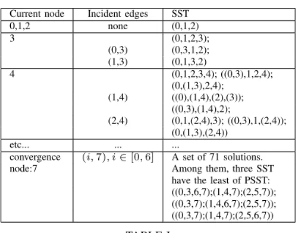
3) Case study: We apply the DPA to the DAG of the
figure 1 and we build the exhaustive list of SST, step by step as described in table I.
B. Depth first search algorithm
Since the solutions set size grows very quickly, we need a much lighter algorithm. Indeed the DPA keeps the exhaustive set of solutions to compute the next set while iterating the following node. Hence, there is a combinatorial explosion and the memory is saturated.
To fix this problem, we propose a depth first search algorithm (DFA) which computes directly the optimal solu-tions. The DFA provides two major advantages; on the one
Current node Incident edges SST 0,1,2 none (0,1,2) 3 (0,1,2,3); (0,3) (0,3,1,2); (1,3) (0,1,3,2) 4 (0,1,2,3,4); ((0,3),1,2,4); (0,(1,3),2,4); (1,4) ((0),(1,4),(2),(3)); ((0,3),(1,4),2); (2,4) (0,1,(2,4),3); ((0,3),1,(2,4)); (0,(1,3),(2,4)) etc... ... ...
convergence (i, 7), i ∈ [0, 6] A set of 71 solutions. node:7 Among them, three SST
have the least of PSST: ((0,3,6,7);(1,4,7);(2,5,7)); ((0,3,7);(1,4,6,7);(2,5,7)); ((0,3,7);(1,4,7);(2,5,6,7))
TABLE I
STEPS OF THEDPAAPPLIED ON THEDAGOF FIGURE1
hand, it needs a little and constant memory consumption (it writes directly the solutions on the disk), on the other hand it converges directly to the optimal solutions. Hence, we are able to exhaustively enumerate the optimal solutions (in terms of SST branches) ordered in travelled times or distances, or to store the optimal solution only. N.B. We use the same input data, as explained in (III-A.2.c).
pkp 0 1 2 3 4 5 6 nv 0 1 2 0 1 2 1
TABLE II
REPRESENTATION OF A SOLUTION TO THEDAGOF FIGURE1
1) Implementation:
a) Chosen representation: We define a solution as an
uni-dimensional array, where each cell represents a pick-up point and where the value of this cell identifies the vehicle serving this point. So, the table size corresponds to the number of pick-up points (nbpkp) minus the convergent
point, i.e.nbgenes = nbpkp− 1. Table II gives a solution of
the picking-up of the CG of figure 1. It corresponds to SST ((0, 3, 7); (1, 4, 6, 7); (2, 5, 7)). Vehicles are indexed from 0 tonbv− 1 where nbv is the number of required vehicles to
solve the CDRTP.
b) Definitions:
CurSolution : current solution to evaluate
BestSolution : best solution found during the process index : node index
nbNodes : number of nodes in the graph VS : useable vehicles set
LVP : Last Vehicles positions (node id)
IsSSTok() : function determining whether a SST is right or
not
Cost() : function giving the time or distance cost of a SST f() : function called recursively on new node
c) Algorithm: f (CurSolution, index, nbNodes, BestSolution, LVP) 1) if index> nbNodes then
a) if Cost(CurSolution)< Cost(BestSolution) then b) BestSolution← CurSolution
2) else
a) VS(index)← {CurSolution[index]|i ∈ Pred{index}} b) for k from 1 to card(VS(index)) do
i) CurSolution(index)← VS(index)(k) ii) if IsSSTok(CurSolution,index)=true then
• if Cost(CurSolution,index)< Cost(BestSolution) then
– LastVehiclePosition(CurSolution(index))← index – f (CurSolution,index+1,nbNodes,BestSolution, LVP)
• endif
iii) endif 3) endif
2) Case study: Let the DFA proceed on the example of
figure 1 (cf. table III). In this case, the heuristic qualify-ing a good solution is the vehicles number, that we aim to minimize. By default, we initialize each node with a different vehicle number, so that the first best solution is ((0,7),(1,7),(2,7),(3,7),(4,7),(5,7),(6,7)).
Current vehicles VS SST Correct node arrangement or better?
init 0 1 2 a b c d better 3 0 1 2 0 b c d (0,1,2,3) ((0,3),(1),(2)) better 4 0 1 2 0 0 c d (0,1,2,3) ((0,3,4),(1),(2)) false 4 0 1 2 0 1 c d (1,2,3) ((0,3),(1,4),(2)) ok 5 0 1 2 0 1 0 d (0,1,2,3) ((0,3,5),(1,4),(2)) false 5 0 1 2 0 1 1 d (1,2,3) ((0,3),(1,4,5),(2)) false 5 0 1 2 0 1 2 d (2,3) ((0,3),(1,4),(2,5)) ok 6 0 1 2 0 1 2 0 (0,1,2,3) ((0,3,6),(1,4),(2,5)) ok 6 0 1 2 0 1 2 1 (1,2,3) ((0,3),(1,4,6),(2,5)) ok 6 0 1 2 0 1 2 2 (2,3) ((0,3),(1,4),(2,5,6)) ok 6 0 1 2 0 1 2 3 (3) ((0,3),(1,4),(2,5),(6)) worse 5 0 1 2 0 1 3 d (3) ((0,3),(1,4),(2),(5)) worse 4 0 1 2 0 2 c d (2,3) ((0,3),(1),(2,4)) ok 5 0 1 2 0 2 0 d (0,1,2,3) ((0,3,5),(1),(2,4)) false 5 0 1 2 0 2 1 d (1,2,3) ((0,3),(1,5),(2,4)) false 5 0 1 2 0 2 2 d (2,3) ((0,3),(1),(2,4,5)) false 5 0 1 2 0 2 3 d (3) ((0,3),(1),(2,4),(5)) worse 4 0 1 2 0 3 c d (3) ((0,3),(1),(2),(4)) worse etc... ... ... ... ... TABLE III
STEPS OF THEDFAAPPLIED ON THEDAGOF FIGURE1
C. Heuristic approach
Because of the combinatorial explosion, we develop meth-ods to approximate solutions in an acceptable computation time. The solution we propose is a genetic algorithm based on the steady state genetic algorithm (SSGA). This one creates a population by cloning the initial genome. At each generation, it creates a temporary population, adds it to the already existing population, then removes the less interesting individuals (those whose fitness is the smallest) to get back to the initial size of population.
1) Objective definition: Let us define a standard solution
and above all, what is a good solution in our study. First, we see the representation we have chosen. We see next how we initialize the population. Then we will see the objective function of our problem.
a) Representation of a solution: We keep the
repre-sentation used in the case of the DFA. Indeed, a solution chromosome is also represented as an uni-dimensional array, where each cell (pick-up point) corresponds to a gene, and the gene value corresponds to the vehicle index serving this point. So, table II represents also a solution chromosome to the CDRT problem of the figure 1.
b) Initialization of the population: The number of
vehicles cannot be greater than the number of pick-up points (nbpkp) and there are at least as many vehicles (nbv) as
initial pick-up points (pkpstart), i.e. minimal nodes of the
CG: nbpkp ≥ nbv ≥ nbpkpstart. We randomly initialize
1000 individuals by assigning a vehicle number among [0, nbpkp]. Thus the start population has a number of not viable
individuals (i.e. wrong solutions). Then the crossover and the objective contribute to improve the solutions. N.B: for each chosen solution, there will be necessarily a different vehicle for each initial pick-up points. So, it may appear more interesting to arrange the table so that the minimal nodes are located ”at the left” of the table. That is, each minimal node from 0 to k is respectively served by a vehicle numbered from 0 tok:∀pkpmini, nvi = i, i ∈ N
c) Objective: If the nodes are correctly ordered, a
good solution consists in checking that the chromosome responds to the following condition:∀i, j, i < j, gene(i) = gene(j) ⇒ ∃(i, j) ∈ E, Hpkpi+ti→j ≤ Hpdrj, whereHpkpi
is the picking up time for the point i. The chromosome fitness increases when it satisfies this condition, favouring the solutions requiring less vehicles, that is, a good solution minimizes the number of PSST. In the contrary, the chromo-some fitness is reduced relatively to the error rate (another solution consists to give fitness 0).
d) Crossover operator: Given that we have a different
vehicle for each initial pick-up point, all chromosomes start with the same common subsequence S. So, to cross two individuals, it is not necessary to span this subsequenceS. The crossover must occur at least from the first gene located over S. Let gS be the first gene located over the common
subsequenceS.
Our crossover operator is parent of the PMX operator [8] and generates two children from two parents. The crossover is simply completed [10] by choosing two random cross points and by swapping sequences of the parents. For exam-ple, in the case of chromosomes P1 and P2 (cf. table IV), we choose a first random numberk, gS≤ k ≤ n, corresponding
to the start of the sequence to swap. We choose a second random number l, k < l ≤ n. Then we create two children C1 and C2 from parents P1 and P2 by swapping the sequences(kl)P 1 and(kl)P 2 (cf. tables IV and V).
0 1 . . . i j k l m n 0 1 . . . i x z w y v 0 1 . . . i j k l m n 0 1 . . . i w v y z x
TABLE IV
PARENTS CHROMOSOMESP1ANDP2
0 1 . . . i j k l m n 0 1 . . . i x v y y v 0 1 . . . i j k l m n 0 1 . . . i w z w z x
TABLE V
CHILDREN CHROMOSOMESC1ANDC2
e) Mutation operator: Mutation aims at bringing
di-versity into the current population. It is a random process, completed from gene gS. So, we assign a random value to
a randomly chosen gene, modulo the number of vehicles in chromosomeC, so that we do not increase the number of required vehicles:∀gene(i) ≥ gS, gene(i) ≤ gene(|C| − 1)
andgene(i) ← (gene(i) + valrnd)%nbvch.
Let us apply the mutation to chromosomeI (table VI); if we randomly choose genek, and we add the random value vrnd = 2 to gene(k), gene(k) ← gene(k) + vrnd, we get
gene(k) = z. After having applied modulo z, z = nbvI, we
get (gene(k) ← gene(k)%z) = 0.
0 1 . . . i j k l m n 0 1 . . . i x x w y v 0 1 . . . i j k l m n 0 1 . . . i x 0 w y v
TABLE VI
EXAMPLE OF MUTATION OF GENEkOF INDIVIDUALI
IV. EXPERIMENTAL RESULTS
We compare the algorithms described above and we pro-ceed the computation of the SST on various CG of increasing sizes (hand-made and randomly generated). We programmed our algorithms in C++ on a PC (2.4GHz with 4GB of memory) running Linux Debian with kernel 2.6. Table VII presents the computation times obtained and highlights the interest of the exhaustive method for CDRT problems with size smaller than 17 pick-up points. Let us note some elements of the k − P D N − T SP complexity. When the QoS constraints and the total order of the graph nodes are not taken into account, the complexity corresponds to generating all combinations of features in a set ofn features (O(2n−1×n!)). By bounding the paths computation, we can
limit complexity between O(2n) and O(2an), with a > 1 and n ≥ 5. For example, if we have a CG G with 7 nodes |G| = 7, the complexity equals to 203. Thus, for a great number of nodes, we need to use another kind of algorithms, such as meta-heuristic algorithms and more especially genetic algorithms.
The genetic application is programmed with the Genetic
Algorithm library (GAlib) developped by the MIT [15]. We
use an initial population size of 1000 indivuals randomly initialized with a crossover ratepcross= 1.0. Each result for
one mutation rate is an average data completed on a series of 100 processes. This algorithm provides a set of representative solutions of good quality, in an acceptable computation time. The convergence speed, with the pertinence of the operators and an appropriate parameterizing, allows to consider appli-cations of size close to several dozens of nodes.
We are interested in the effects of the variation of the mutation rate pmut. We vary pmut from 0.0001 to 0.9 on
a population of 1000 individuals, by solving the CDRT problem on CG with 20, 30, 40 vertices. Table VIII presents results obtained from these graphs,|S| is the average number
of different solutions and Dbs indicates the average
per-centage of the different sub-optimal solutions obtained on these graphs. Globally, by increasing the mutation rate, we increase the number of various solutions. From a mutation ratepmut 0.1, there is no more significant increase of the
number of distinct solutions. Moreover, the more important the graph density, the stronger the mutation rate, if we expect a solution quickly. Indeed, it is only from a mutation rate around 0.1, that the whole solutions are sub-optimal, whereas in the case of smaller graphs (20, 30 nodes), the population has large sets of sub-optimal solutions with weaker mutation rates (pmut≤ 0.05).
We are now interested in the convergence speed and we want to know from which generation the first sub-optimal solution appears. Generally, the more the mutation rate in-creases, the faster we get a sub-optimal solution (cf. figure 2). The first sub-optimal solution occurring has to be correlated with the number of nodes and the edges density. Thus, for small dimension problems like graphs with 20, 25 nodes, we get an optimal solution very quickly (before around 30 generations in average) for a mutation ratepmut<0.05. But,
as soon as we increase a little bit the nodes and edges density (30 nodes), the first sub-optimal solution appears very later for a similar mutation rate (around 600 generations). In the case of the 30 nodes graph, it requires a mutation rate pmut ≥ 0.05 to find a sub-optimal solution before 200
generations! The algorithm may find a sub-optimal solution to the 30 nodes graph problem in around 30 generations with a stronger mutation rate only (pmut≥ 0.3).
Our research group made a recent survey in France and recorded about 650 DRTs. This can give us an idea of how useful can be our algorithms. We are indeed able to know, for about 100 of them that are CDRT, the number of clients that requested a trip for the same time [4]. A large part of these DRTs only serves about 10 clients per round. For those, the exact solutions provided by the DPA or the DFA could be sufficient. Other services manage less than 20 clients, allowing to use the DFA algorithm. However, sometimes for these services and often for a few efficient
Number Number CPU time CPU time CPU time of node of edges with DPA with DFA with GA
8 18 0 0 4.56 12 41 0.01 0.01 5.56 13 44 0.04 0.02 5.82 14 54 0.31 0.12 6.21 16 73 8.17 2.15 6.64 23 176 - 950.65 10.74 25 247 - - 11.79 30 391 - - 15.35 40 743 - - 27.65 50 1156 - - 65.88 60 1693 - - 90.71 70 2305 - - 116.94 80 3011 - - 161.06 90 3821 - - 215.83 100 4825 - - 268.98 200 19569 - - 1602.02 TABLE VII COMPUTATION TIMES OFSST
pmut CG20 CG30 CG40 |S| Dbs |S| Dbs |S| Dbs 0.0001 29.0 90 103.3 80 8.9 0 0.0005 43.9 80 144.5 30 72.4 0 0.001 26.0 70 194.5 30 34.3 0 0.005 101.9 100 394.0 70 355.7 0 0.01 165.1 100 696.4 70 586.6 0 0.05 619.8 100 971.4 100 832.7 30 0.1 767.0 90 980.7 90 793.3 80 0.2 852.0 100 981.1 100 848.0 90 0.3 863.4 100 977.1 100 857.5 100 0.4 882.2 100 981.0 100 869.1 100 0.5 887.2 100 981.7 100 873.4 100 0.6 896.0 100 983.1 100 896.1 100 0.7 907.2 100 981.7 100 905.1 100 0.8 918.1 100 984.9 100 918.9 100 0.9 925.1 100 987.4 100 935.5 100 TABLE VIII
VARIATION OF NUMBER OF DIFFERENT SOLUTIONS
0 100 200 300 400 500 600 700 800 900 1000 0 0.1 0.2 0.3 0.4 0.5 0.6 0.7 0.8 0.9 Generation Mutation rate 20 nodes 25 nodes 30 nodes
Fig. 2. Average generations of appearing of the first sub-optimal solution
CDRT, the number of clients exceeds 30. The GA, despite a decreasing efficiency, remains the best solution for that range of services.
V. CONCLUSION AND FUTURE WORK
This paper presents three algorithms, two exact ones and an heuristic one. Both of them constitute the cornerstone of a CDRT solution by solving the problem of scalability. Moreover these algorithms, which solve various kinds of the general P&D TSP, provide flexibility to the system. The implementation provides pragmatic solutions to np-complete CDRT problem. The efficiency of these algorithms is obtained thanks to constructed objects (transitive graph), and computed objects (SST that represent the solutions integrating the QoS constraints). The total order on the nodes of a convergent graph implies the efficiency experimentally observed on an one-step run of the DPA∞-PD N-TSP, and the fast convergence of our parameterized SSGA.
According to the graph density and thus to the solving complexity, we can choose the most appropriate solving method, so that our system is still able to satisfy the users requests and the carriers constraints. Our further works will intend to adapt the system by choosing the appropriate algorithm solving a CDRT operating in real-time conditions and assess the corresponding complexity.
Tested experiments lead us to pursue on two ways. First, DPA and DFA face to the scalability problem. So we are
able to improve these algorithms by integrating heuristics like capacity or travel times and to develop the flexibility of our solutions. Second, we can improve the GA for larger flows and refine the solutions with a new set of constraints.
REFERENCES
[1] G. Ambrosino, J. Nelson, and M. Romnazzo. Demand Responsive
Transport Services: Towards the flexible Mobility Agency. Rome: ENEA, 2004. 325 p.
[2] B. Julstrom and G. Raidl. Initialization is robust in evolutionary
algorithms that encode spanning trees as sets of edges. In Symposium
on Applied Computing, pages 547–552. ACM Press, 2002.
[3] Bryant A. Julstrom and G¨unther R. Raidl. A permutation-coded
evolutionary algorithm for bounded-diameter minimum spanning tree
problem. In 2003 Genetic and Evolutionary Computation
Confer-ence’s Workshops Proceedings, Workshop on Analysis And Design of Representations, 2003.
[4] E. Castex, R. Chevrier, D. Josselin, and P. Canalda. Le transport la demande en multi-convergence. In SAGEO’06, Strasbourg, France, sep 2006. 13 pages, to be published.
[5] P. Chalasani and R. Motwani. Approximating capacitated routing and delivery problems. Technical report, Stanford University, 1995. [6] R. Chevrier, P. Canalda, P. Chatonnay, and D. Josselin. An oriented
convergent mutation operator for solving a scalable convergent demand
responsive transport problem. In ICSSSM’06, IEEE Int. Conf. on
Service Systems and Service Management, Troyes, France, Oct. 2006.
6 pages, to be published.
[7] R. Chevrier, P. Canalda, P. Chatonnay, and D. Josselin. Vers une
solution robuste et flexible du transport `a la demande en convergence : ´etude trans-disciplinaire et mise en oeuvre. In Actes du Workshop
International : Logistique et Transport 2006 (LT 2006), pages 49–55,
Hammamet, Tunisie, Apr. 2006.
[8] D. Goldberg. Genetic algorithms in search, optimization, and machine
learning. Addison-Wesley, 1989.
[9] D. Montana, M. Brinn, G. Bidwell, and S. Moore. Genetic algorithms for complex, real-time scheduling. In IEEE Conference on Systems,
Man and Cybernetics, volume 3, pages 2213–2218, 1998.
[10] D. Whitley. A genetic algorithm tutorial. Statistics and Computing, 4:65–85, 1994.
[11] G¨unther R. Raidl and Bryant A. Julstrom. Greedy heuristics and an evolutionary algorithm for the bounded-diameter minimum spanning tree problem. In SAC ’03: Proceedings of the 2003 ACM symposium
on Applied computing, pages 747–752, New York, NY, USA, 2003.
ACM Press.
[12] K.A. DeJong and W.M. Spears. Using genetic algorithms to solve
np-complete problems. In Proceedings of the Third International
Conference on Genetic Algorithms, pages 124–132, 1989.
[13] M. Bielli, M. Caramia, and P. Carotenuto. Genetic algorithms in bus network optimization. Transportation Research, C:19–34, 2002. [14] M. Forbes. Capacitated vehicle routing and the k-delivery n-traveling
salesman problem. Master’s thesis, Montgomery BlairHigh School, 2004.
[15] M. Wall. Genetic algorithm library. http://lancet.mit.edu/ga/. [16] M.E.T. Horn. Fleet scheduling and dispatching for demand-responsive
passenger services. Transportation Research, 10(1):35–63, 2002.
[17] M.W.P. Savelsberg and M. Sol. The general pickup and delivery
problem. Transportation Science, 1(29):17–29, 1995.
[18] N. Christophides, A. Mingozzi, and P. Toth. Exact algorithms for solving the vehicle routing problem based on spanning trees and shortest path relaxations. Mathematical Programming, 20:255–282, 1981.
[19] Olli Br¨aysy and Michel Gendreau. Vehicle routing problem with time windows, part I and II. Transportation Science, 39(1):104–118 and 119–139, 2005.
[20] J. Renaud, F. F. Boctor, and J. Ouenniche. A heuristic for the
pickup and delivery traveling salesman problem. Comput. Oper. Res., 27(9):905–916, 2000.
[21] S. Arora. Polynomial time approximation schemes for Euclidean
traveling salesman and other geometric problems. Journal of the ACM, 45(5):753–782, 1998.
[22] TCRP, D. Koffman. Operational experiences with flexible
tran-sit services, a synthesis of trantran-sit practice. Technical
re-port, Washington : National Academy Press, Aug. 2004. 71p.,
http://www.trb.org/publications/tcrp/tcrp syn 53.pdf.