HAL Id: hal-01311309
https://hal.sorbonne-universite.fr/hal-01311309
Submitted on 4 May 2016
HAL is a multi-disciplinary open access
archive for the deposit and dissemination of
sci-entific research documents, whether they are
pub-lished or not. The documents may come from
L’archive ouverte pluridisciplinaire HAL, est
destinée au dépôt et à la diffusion de documents
scientifiques de niveau recherche, publiés ou non,
émanant des établissements d’enseignement et de
Line parameter study of ozone at 5 and 10µm using
atmospheric FTIR spectra from the ground: A
spectroscopic database and wavelength region
comparison
Christof Janssen, Corinne Boursier, Pascal Jeseck, Yao Té
To cite this version:
Christof Janssen, Corinne Boursier, Pascal Jeseck, Yao Té.
Line parameter study of ozone at
5 and 10µm using atmospheric FTIR spectra from the ground: A spectroscopic database and
wavelength region comparison. Journal of Molecular Spectroscopy, Elsevier, 2016, 326, pp.48-59.
�10.1016/j.jms.2016.04.003�. �hal-01311309�
Line parameter study of ozone at 5 and 10 µm using
atmospheric FTIR spectra from the ground:
A spectroscopic database and wavelength region
comparison
Christof Janssena,∗, Corinne Boursiera, Pascal Jesecka, Yao T´ea aLERMA-IPSL, Sorbonne Universit´es, UPMC Univ Paris 6, Observatoire de Paris, PSL Research
University, CNRS, F-75005, Paris, France
Abstract
Atmospheric ozone concentration measurements mostly depend on spectroscopic meth-ods that cover different spectral regions. Despite long years of measurement efforts, the uncertainty goal of 1% in absolute line intensities has not been reached yet. Mul-tispectral inter-comparisons using both laboratory and atmospheric studies reveal that important discrepancies exist when ozone columns are retrieved in different spectral regions. Here, we use ground based FTIR to study the sensitivity of ozone columns on different spectroscopic parameters as a function of individual bands for identify-ing necessary improvements of the spectroscopic databases. In particular, we examine the degree of consistency that can be reached in ozone retrievals using spectral win-dows in the 5 and 10 µm bands of ozone. Based on the atmospheric spectra, a detailed database inter-comparison between HITRAN (version 2012), GEISA (version 2011) and S&MPO (as retrieved from the website at the end of 2015) is made. Data from the 10 µm window are consistent to better than 1%, but there are larger differences when the windows at 5 µm are included. The 5 µm results agree with the results from 10 µm within±2 % for all databases. Recent S&MPO data are even more consistent with the desired level of 1 %, but spectroscopic data from HITRAN give about 4% higher ozone columns than those from GEISA. If four sub-windows in the 5 µm band are checked for
∗corresponding author
consistency, retrievals using GEISA or S&MPO parameters show less dispersion than those using HITRAN, where one window in the P-branch of theν1+ ν3 band gives
about 2 % lower results than the other three. The atmospheric observations are corrob-orated by a direct comparison of the spectroscopic databases, using a simple statistical analysis based on intensity weighted spectroscopic parameters. The bias introduced by the weighted average approach is investigated and it is negligible if relative di ffer-ences between databases do not correlate with line intensities. This is the case for the comparison of HITRAN with GEISA in the 10 µm region and the agreement between the simple analysis and the full retrieval is better than 0.1%. At 5 µm biases might be as high as 1.4 %, and the proposed method is thus limited to the same level of accu-racy. Implications of the new data for database improvements and further studies, in particular in the 5 µm region, are discussed.
Keywords: ozone, atmospheric composition, remote sensing, FTIR, MIR, spectroscopic database
1. Introduction
The triatomic allotrope of oxygen, ozone (O3), is a key molecule in Earths
atmo-sphere. As precursor molecule for atmospheric radicals (NO3, OH) it plays a central
role in atmospheric oxidation. Ozone also filters harmful solar ultraviolet (UV) radia-tion and thus is crucial to the evoluradia-tion of life as we know it. The molecule has direct
5
impact on air quality, agricultural productivity, and the ecosystem with correspond-ing economic consequences. Accurate and traceable concentration measurements of this molecule thus are a priority for health and air quality authorities as well as for atmospheric and climate scientists, which has made ozone one of the key themes of dedicated global atmospheric observation programs, such as IGACO-O3/UV.1
10
1Integrated Global Atmospheric Chemistry Observations for ozone and UV as part of the Global
Atmo-spheric Watch (GAW) Programme of the World Meteorological Organisation for providing reliable scientific data and information on the chemical composition of the atmosphere, its natural and anthropogenic change, and helping to improve the understanding of interactions between the atmosphere, the oceans and the bio-sphere.
Due to its high reactivity and the impossibility to prepare a stable reference standard along with the fact that ozone has rich and strong absorption features covering all spec-tral regions from the far IR to the UV, O3concentration measurements are commonly
based on spectroscopic methods. These measurements thus depend on the molecular spectroscopic constants describing the interaction with light, which have to be
deter-15
mined experimentally. Indeed, the recommended primary method for in-situ ozone measurements in ambient air hinges on the absorption cross section in the Hartley band at 253.65 nm, whose actually recommended value suffers from a relative uncertainty of 2.1 % (at the 95 % level of confidence) [1]. In view of the need for reliable long term measurements of ozone changes of a few percent per decade [2–5], traceable
spectro-20
scopic data with a much lower level of uncertainty are desired and redeterminations of this cross section value are thus under way [6–8]. A target uncertainty for concentration measurements and remote sensing of atmospheric ozone is one percent [1, 7, 9, 10], or below. This would also allow meaningful retrieval of tropospheric ozone from satellite data where the total column is dominated by the stratospheric contribution (∼ 90 %).
25
Achieving and well characterizing this level of uncertainty will also make an important contribution to the United Nations effort in documenting long-term ozone trends [11].
In order to harmonize the spectroscopic data on ozone, the most recent mid-IR intensity studies in the 10 µm range [2–5, 12–15] have been critically reviewed [16] and the databases have been updated concordantly after 2004 [17–19]. Because three
30
of four recent measurements showed a dispersion of just±0.8%, it was recommended to reduce the database values by roughly 4 % which corresponded to the average of the three consistent data sets. The recommendation thus has effectively ignored the recent measurement of Smith et al. [12] even though it was consistent with previous measurements and the actual recommendation (HITRAN 2000) at that time and this
35
was done without pointing out why this particular measurement should be less reliable than the other studies.
Interestingly, recent direct UV (300-315 nm) - IR (10 µm) inter-comparison mea-surements in the laboratory [20, 21], in the atmosphere from ground [22] or using satellite instruments [23] have questioned the thus obtained consistency of the updated
40
often find a difference of about 4 % in the derived ozone concentrations or columns. This could possibly indicate that the original HITRAN 2000 database [24] values are more consistent with recommended UV data. A similar difference of (3.6 ± 1.0) % has been found in another UV - IR inter-comparison based on simultaneous measurements
45
at the Hg emission line at 253.65 nm and around 1133.5 cm-1in theν1band [25].
More-over, using the same two databases (HITRAN 2004 or 2008), the ACE-FTS mission team has decided to neglect the results from ozone spectroscopic data in the 5 µm band (in theν1+ν2band around 1800 cm-1and in theν1+ν3band around 2100 cm-1), because
of apparent discrepancies with the results obtained from retrieval in the 10 µm
funda-50
mental region [23]. This has triggered another inter-comparison study [26] between the integrated absorption in the Chappuis band (515 - 715 nm) and theν1+ ν3combination
band. There, however, no inconsistencies in recommended databases have been found, but optical densities in the visible were very weak though (< 4 %). Thomas et al. [27] studied recently possible inconsistencies between the 5 and 10 µm regions by absolute
55
measurements in each of these two regions. Their results at 10 µm are compatible with the 2004 or 2008 HITRAN databases and about 2 % lower than the actual databases in the 5 µm region, which, if significant, could even increase the observed discrepancy in the satellite data [23, 28].
Very recently, the first direct inter-comparison between the 3 and 10 µm as well
60
as the 4 and 10 µm regions has been published [29]. This study is based on ground based FTIR solar absorption spectra and systematic differences of up to 7 % between the different regions have been revealed, most likely due to inconsistencies in the spec-troscopic data.
Given these many seemingly conflicting results, further inter-comparisons, ideally
65
using identical conditions for the ozone concentration and the optical light path, are sought for. Besides of the inherent difficulty to prepare ozone for comparison and absolute intensity measurements, some of the discrepancies are certainly due to the use of different lines and spectral regions. In this article we thus try to investigate the consistency of the 5 µm data with the 10 µm region: i) globally, as a function of
70
the vibrational band and ii) locally, as a function of few individual transitions, using atmospheric observations from a ground based FTIR instrument. The present study
thus is part of a greater effort of using ground based atmospheric remote sensing studies for improving the spectroscopic databases, such as has been demonstrated for the case of water [30], for example.
75
Our comparisons are done using the currently available data from the three different spectroscopic databases GEISA [31], HITRAN [32] and S&MPO [33], which allows one to investigate differences and possible inconsistencies. Due to the complexity of linking column measurements to spectroscopic data, a simple method is introduced that permits to derive characteristic spectroscopic parameters for each spectral window
80
and database. Based on comparisons of these representative values, differences in at-mospheric retrievals can be traced back to differences in the spectroscopic databases. The comparison of databases in each of the spectral regions is thus another goal of this article, which is structured as follows: We begin with a description of the experimen-tal tools, the spectroscopic data and the retrieval procedure. The sensitivity of ozone
85
columns on different spectroscopic parameters in the 10 µm range is then discussed and we conclude with a detailed comparison of ozone data in the spectroscopic databases in the light of our measurements.
2. Experimental setup and data
2.1. Observation site and instrumental description
90
Atmospheric observations were performed using the Paris ground-based Fourier transform spectrometer (FTS-Paris). This instrument is operated by the SMILE/LERMA2 team and is part of the QualAir air quality research station of Universit´e Pierre et Marie Curie (UPMC). The instrument is located in downtown Paris on the UPMC campus (48◦50’N, 2◦21’E at 65 m a.s.l). A detailed description of the system can be found
95
elsewhere [34]. Here, we just give a short description and technical key data are sum-marized in Table 1.
2SMILE is the French acronym for ”Molecular Spectroscopy and Laser Instrumentation for the
2.2. Data acquisition
The spectra recorded by ground-based FTIR contain rovibrational signatures of atmospheric species in the characteristic fingerprint and group frequency regions (3−
100
10 µm, extendable). To optimize the signal-to-noise ratio in the spectral domains of the ozone signals, appropriate combinations of optical filters and detectors have been chosen (see Table 1). Data were acquired during daytime and only clear sky spectra have been kept for the analysis. In order to optimize the signal-to-noise ratio, the evaluation has further been restricted to spectra that were obtained around noon (10:00
105
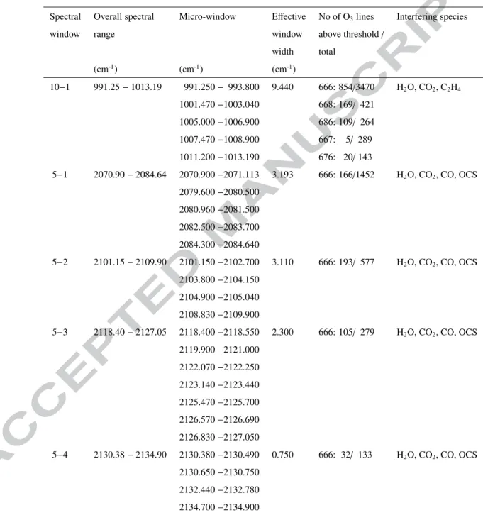
– 14:00). Here we present data that were acquired at six days in 2013. An overview of the spectroscopic data and windows is given in Figure 1.
2.3. Spectroscopic Data
Data were taken from the latest versions of the three databases GEISA, HITRAN and S&MPO (G11, H12 and S15, hereafter). The origin of these data and the
avail-110
able parameters are specified for each spectral region separately. Note that S&MPO does not keep track of changes of the available data. The data used here represent a snapshot made in December 2015 using the smpo.univ-reims.fr website. All of the databases essentially provide spectroscopic data concerning the main and singly sub-stituted ozone species: 16O
3, 16O16O18O,16O18O16O,16O16O17O,16O17O16 (or 666, 115
668, 686, 667, 676 in shorthand notation). While the singly substituted isotopologues except for16O18O16O have been included into the database only at the end of 2015,
S15 also includes the pure18O3 isotopologue and gives intensities on a per species’
basis. H12 and G11 assume that the above molecules occur in fixed proportions of 0.992901, 0.00398194, 0.00199097, 0.000734 and 0.00370 respectively [24]. These
120
relative abundance factors are therefore already incorporated into intensities given in the databases [35], which is also the convention assumed by the retrieval software. The above relative values are based on the isotope abundance of standard mean ocean wa-ter (SMOW) [36]. By taking these proportions one evidently ignores the strong and variable isotopic enrichments that actually occur in atmospheric ozone [37–39].
Nev-125
ertheless, the assumption is made throughout and will have no significant impact on the total ozone column values.
Another notable difference between databases is the kind of spectroscopic param-eters that are provided. Table 2 gives a comparison of these data. The lack of the air temperature coefficient nairof the broadened half width in S&MPO needs to be pointed 130
out here as a possible obstacle for atmospheric applications. Throughout the paper we have assumed the constant value nair = 0.76 in doing retrievals with S15. As far as
line intensities of16O
3 are concerned, data from the{ν1,ν3} fundamentals at 10 µm
in H12 and S15 are due to dipole moments of Flaud et al. [16] (see Ref. [40]), while corresponding values in G11 are referenced to Ref. [14]. The 5 µm cold band
transi-135
tions of16O
3in H12 stem from the calulation published in Ref. [41] and are scaled by
a normalization factor of 1/(1.04) [40]. The same data in G11 result from the work in Ref. [42], while corresponding transitions in S15 come from calculations of GSMA in Reims [43].
The 10 µm region comprises the fundamental of the dyad formed by the normal
140
stretch modes ν1 andν3, but also harmonic and hot band transitions. We note that
normal mode frequencies are 1103.08 and 1041.89 cm-1forν1andν3, respectively and
that theν3band has the highest band intensity of the normal modes. Altogether 1157
lines in the selected window 10−1 at and above our threshold intensity of 10−23cm are reported in HITRAN.
145
The threshold, which was not applied to the retrieval that included all available lines in the databases, corresponds to 2 to 3 times our limit of detection (LOD). These lines belong to different vibrational transitions. Using the Boltzmann factors
FB(T )= exp(−c2E′′/T), (1)
defined by the lower state energy E′′, temperature T and second radiation constant c2 = 1.4387770(13) K cm1, one readily estimates that only ground state{001, 100} ← 150
000 and hot band transitions from the first excited states 010, 001 and 100 need to be considered at 296 K, if contributions of less than 0.2 % to the total intensity are ne-glected. The restriction to the above transitions should even be more accurate, because temperatures in the ozone layer are much lower.
2.3.1. Retrieval strategy
155
Ozone total columns
CO3=
∫
nO3(z) dz (2)
where nO3(z) is the ozone number density along the light path with coordinate z, are
retrieved using the PROFILE FIT (PROFFIT) algorithm developed by Hase et al. [44]. The radiative algorithm (forward model) is based on the Beer-Lambert law and calcu-lates the atmospheric absorbance, which is compared and fitted to the measured
spec-160
trum using a least squares minimization method. Input parameters for the forward modeling are: spectroscopic line parameters (position, intensity, pressure line shift, pressure broadening parameters) from the spectroscopic databases; atmospheric pres-sure and temperature vertical profiles from NOAA (see http://www.ncep.noaa.gov); a priori vertical Volume Mixing Ratio (VMR) profiles of all of the studied species, the
165
H2O continuum [45], and the instrument line shape [46–48], which is regularly
moni-tored using sealed and non-sealed gas cells filled with HCl, HBr and N2O. The
inver-sion model supports both optimal estimation and Twomey-Tikhonov constraints and is able to perform the retrieval in log(VMR) space for strong variability in an optimal manner. Columns are measured along the light path but are usually converted to
verti-170
cal columns, assuming spherical symmetry of the atmosphere. In this paper we do not need to be concerned with the difference between these two and might for simplicity assume that the absorption occurs along the vertical direction.
In the spectral regions corresponding to the fundamental{ν1,ν3} bands at 10 µm,
one window (10−1) consisting out of 5 sub-windows was used and in the region of
175
theν1+ ν3combination bands at 5 µm four different windows (5−1 through 5−4) with
between 4 and 7 sub or micro-windows were employed in the analysis. The windows and the micro-windows are detailed in Table 3 and Figure 2 gives a graphical repre-sentation of the acquired spectra. Micro-windows in both spectral ranges were chosen in order to minimizing contributions from interfering species, which mainly are H2O, 180
CO2, N2O, CO and OCS. Their contributions were determined in separate retrievals
using appropriate spectral windows. The ozone columns have then be retrieved using a daily mean vertical profile of the interferer substances.
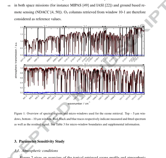
We note that the 10 µm range has been used intensively for the retrieval of ozone in both space missions (for instance MIPAS [49] and IASI [22]) and ground based
re-185
mote sensing (NDACC [4, 50]). O3columns retrieved from window 10-1 are therefore
considered as reference values.
Figure 1: Overview of spectral regions and micro-windows used for the ozone retrieval. Top – 5 µm win-dows, bottom – 10 µm window. Red, black and blue traces respectively indicate measured and fitted spectrum as well as the residual signal. See Table 3 for micro-window boundaries and supplemental information.
3. Parameter Sensitivity Study
3.1. Atmospheric conditions
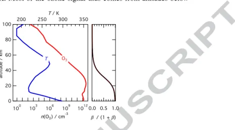
Figure 2 gives an overview of the typical retrieved ozone profile and atmospheric
190
measurement conditions. In the altitude range from 0 to 34 km, ozone number densi-ties vary between 0.9 and 4· 1012cm-3, with the maximum reached at circa 23 km of
altitude. Above 34 km, ozone concentrations decrease exponentially at a rate of about one decade per 7 km. Temperatures at the ozone maximum are on the order of 220 K and the column averaged ozone temperature
195 TO3= ∫ dz T (z) nO3(z) ∫ dz nO3(z) (3)
takes the value of 235 K. Most of the ozone signal thus comes from altitudes below
Figure 2: Typical ozone and temperature profiles of measurements in 2013 (left panel). Right panel shows β/(1 + β), which is an indicator for the contribution of the pressure broadened halfwidth to the overall line width.
34 km. The Voigt shape parameter
β = γL/γG (4)
whereγL andγGare Lorentzian and Gaussian halfwidths, respectively, can be used
to quantify the importance of pressure broadening on the line shape. The function β/(1 + β), in particular, is a measure for the contribution of pressure broadening to the
200
total linewidth. It takes a value of 39 % at 34 km, and increases steadily with decreas-ing altitude, indicatdecreas-ing that pressure broadendecreas-ing is dominatdecreas-ing in the altitude range somewhat below 34 km.
3.2. Sensitivity study at 10 µm
In order to identify spectroscopic requirements and understand differences between
205
spectroscopic databases, we have determined the sensitivity of the ozone columnCO3
to the intensity (S ), air-broadened half width (γair), its temperature coefficient (nair)
and the lower state energy (E′′) expressed as equivalent wavenumber.
Line shape parameters beyond the Voigt profile due to Dicke narrowing, speed effects (velocity changing collisions and speed dependence of pressure broadening and
210
therefore don’t discuss these effects here. Actually, non-Voigt effects on isolated ozone lines can be safely neglected, since their impact on the total ozone column is 0.1 % or less [51]. However, neglecting line-mixing effects can bias the ozone total column retrieval in the 10 µm range by up to 2 % [52], but in section 4 we will present evidence
215
that if any, the impact of line-mixing on total ozone column values in our study is likely significantly smaller (< 1 %).
We here define the sensitivity coefficient α as the proportionality factor between relative changes ofCO3due to relative changes of the respective parameter x∈ (S, γair,
nair, E′′), i.e.: 220 ∆CO3 CO3 = α(x)∆x x . (5)
Related definitions, such as the band specific sensitivityαI(x) and corresponding weight
factors wI are given in Appendix A.1.
Table 4 gives intensity weights wIin the 10 µm window for the bands that account
for more than 99 % of the absorbed intensity at T = 235 K. It indicates that the fun-damentals{001,100} ← 000 should contribute about 93 % to the retrieved signal. The
225
second most important transition is the hot band from theν2= 1 lower state (∼5 %).
Note that calculated weights are only approximate. In the atmosphere, radiation transfer based on the Beer-Lambert law
I(ν) = I0(ν) exp − ∫ nO3(z) ∑ l Sl(z) gl(ν, z) dz (6)
(here given for a single absorber with multiple absorption lines l of line shape gl(ν, z)
and a vertical number density profile nO3(z) and neglecting the apparatus function) 230
will introduce a non-linearity, because the exponential preferentially damps stronger transitions. On the contrary, the averaging in eqs. (A.3) and (A.2) which is used to determine the contribution of individual bands to the overall signal in Table 4, does not take this dampening into account and must therefore overestimate strong absorption lines.
3.2.1. Sensitivity on line intensity
The optical density is defined as the negative of the exponent in the Beer-Lambert law (eq. (6)): τ(ν) = ln ( I0(ν) I(ν) ) = ∫ nO3(z) ∑ l Sl(z) gl(ν, z) dz. (7)
τ is thus linear in both, S and nO3. Since the total ozone column (eq. (2)) is also linear
in nO3, but independent of S , the line intensity andCO3are directly anti-correlated and 240
α(S) = −1. This value (−0.98) is indeed obtained for the sum of all bands (see Table 4). For individual bands, however, some deviation from the average is observed and val-ues between 0.8 and 1.8 times of the average are obtained. As discussed before, the non-linearity of eq. (6) and the simplifying assumption of an isothermal atmosphere contribute to this difference. The ν3 fundamental, in particular, shows a sensitivity 245
|α(S )| < 1, which is in line with the expectation that the band with the strongest tran-sitions should have a sensitivity weaker than average. Evidently, there must be other bands that compensate for this deficit, explaining the relatively large value for the hot band from theν2= 1 lower state.
For the discussion of the sensitivity to other parameters (γair, nair), ratios of
α-250
values are also presented in Table 4.
3.2.2. Sensitivity on pressure broadening coefficient
Inspection of Table 4 reveals that|α(γair)| is roughly three to six times smaller than
|α(S)|. Intensity corrected values |α(γair)/α(S)| are between 0.15 and 0.3. However, a
striking feature in Table 4 is the opposite sign ofα(γair) for 001← 000 as compared to
255
the other vibrational bands. As shown in a simple numerical simulation in Appendix A.2, this is caused by line shape biases which are different for high and low peak center optical densitiesτ0, which must affect the strong 001 ← 000 band differently than the
others.
An empirical correlation between line intensity and peak center optical densityτ0 260
has been derived from the atmospheric spectra (Fig. 1) using some lines around 992 and 1006 cm-1. By comparison with the characteristic intensity of each band (obtained as intensity weighted average, see supplementary material),τ0 ≃ 9 and α(γair)< 0 is
estimated for the 001←000 fundamental, whereas the range 0.08 ≤ τ0 ≤ 0.6
corre-sponding toα(γair)≃ +0.4 is derived for the remaining weak bands (see Fig. A.7e).
265
Due to the simplifying approach of characterizing the bands by their weighted in-tensity and due to using an empirical correlation and ignoring the vertical atmospheric structure, it is not surprising that the agreement between the simple modeling and our observations is only semi-quantitative and that the sensitivity for theν3fundamental is
overestimated by our approach. Nevertheless, the sign change with intensity as well as
270
the sensitivity coefficient |α(γair)/α(S)| ≃ 0.3 in Table 4 for the weak band transitions
is quite well reproduced by the simple estimation. The modeling results thus confirm our interpretation of the sensitivity coefficient being a fitting artefact due to biases in γair.
3.2.3. Sensitivity on temperature coefficient of pressure broadening
275
The temperature coefficient nairdetermines the temperature dependence of the
pres-sure broadening coefficient
γair(T )= γair(296 K) ( 296 K T )nair . (8)
Biases in nairare therefore directly linked to biases inγair, especially if measurements
or observations are made at one particular temperature. We therefore expect that there is a strong correlation between the sensitivity coefficients of these two parameters. The
280
ratio α(γair)/α(nair) for an isothermal atmosphere might be derived from the above
eq. (8) by taking the derivative ofγairwith respect to nairand keeping the lowest order
correction (note that we drop the index air for the moment) ∆γ γ (T ) = ( 296 K T )∆n − 1 ≃ n ln ( 296 K T ) ∆n n . (9)
which directly leads to
α(γ) α(n) ≃ n−1ln−1 ( 296 K T ) . (10)
For the two 011 ← 010 and 002 ← 001 hot bands and the ν1 fundamental, the 285
intensity weighted temperature coefficients nair (see supplementary material). Using
our characteristic ozone temperature from eq. (3) of 235 K and following eq. (10), these values correspond to sensitivity ratiosα (γair)/α (nair) between 5.4 and 6.1 (H12) and
between 5.7 and 5.9 (G11). These ranges are very consistent with the observed range
290
from 5.3 to 5.6 defined by the two strongest of the weak transitions in Table 4. Given the large measurement uncertainties, especially for the weak bands that contribute by only about 1 % to the overall absorption signal, this agreement might be somewhat accidental, as indicated by the value of 4.3 for theν3 hot band, which is somewhat
below the expected range.
295
3.2.4. Sensitivity on lower state energy
The main impact of the lower state energy E′′(or its equivalent wavenumber value) on the intensity, and thus on the ozone column, is via the Boltzmann factor FB(T ) in
eq. (1) [see 35, for example]. It is thus evident that ∆CO3 CO3 = −∆S S = c2 T∆E ′′. (11)
At 235 K, c2/T = 6.1·10−3cm and due to lower state energies being usually known 300
better than 10−2cm-1, the uncertainties in E′′have a negligible (< 10−4) impact on the (relative) uncertainty of the column measurements.
4. Database comparison
4.1. 10 µm region
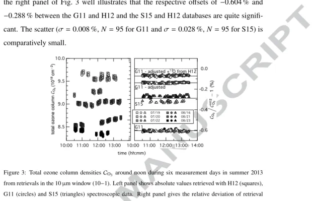
Fig. 3 shows retrieval results for total ozone column densities from the 10 µm
305
region at Paris during six summer days around noon using the G11, H12 and S15 databases. The left panel demonstrates that column density retrievals give similar val-ues when either of the three databases is used. Within one four-hour observation pe-riod, ozone columns are between 8.3 and 9.7 · 1018cm−2and vary only on the 1 % scale (∼ 0.1 · 1018cm−2). However the data reveal a small systematic bias between the three
310
databases. Columns retrieved using the H12 database are always higher than columns from S15 and G11, and retrievals using G11 always give the lowest results. Indeed,
the right panel of Fig. 3 well illustrates that the respective offsets of −0.604 % and −0.288 % between the G11 and H12 and the S15 and H12 databases are quite signifi-cant. The scatter (σ = 0.008 %, N = 95 for G11 and σ = 0.028 %, N = 95 for S15) is
315
comparatively small.
Figure 3: Total ozone column densitiesCO3 around noon during six measurement days in summer 2013
from retrievals in the 10 µm window (10−1). Left panel shows absolute values retrieved with H12 (squares), G11 (circles) and S15 (triangles) spectroscopic data. Right panel gives the relative deviation of retrieval results in percent. Circles and triangles correspond to results with unmodified G11 and S15 spectroscopic data, respectively. Squares are differences when bandwise corrections are applied to16O and18O-containing
ozone in G11. Diamonds indicate deviations when17O data from H12 are added to the modified G11 data.
Most of the bias between G11 and H12 is due to systematic differences in the av-erage spectral parameters. Table 5 demonstrates that some intensity weighted spectral parameters, and even intensity values, differ by several percent. If S, γair and nair in
G11 are thus adjusted bandwise by the ratio xH12/xG11to compensate for these di ffer-320
ences, the relative bias is reduced to a value of only−0.138 % (σ = 0.005 %, N = 95), as shown in the right panel of Fig. 3. Interestingly, correcting for systematic biases be-tween H12 and S15 using the same method does not improve the relative deviation in the column values; at the same time the dispersion of the data is significantly reduced. The results are not shown in Fig. 3, but we get a−0.323 % offset with a σ = 0.007 %
325
dispersion when we apply the standard correction procedure based on the weighted averages in Table 5. The reduction of the dispersion is mainly due to the difference inγair. As a matter of fact, correcting for differences in the weighted averages of γair
using the actual values ofγairin H12 with intensities of S15. In this case the offset is 330
−0.227 % with a standard deviation of σ = 0.007 %. The comparison using the three databases also shows that usingγairfrom either H12 or G11 leads to a small dispersion
in the retrieved columns, whereas the dispersion is about four times higher when S15 is compared to H12. Note, that relative differences in weighted γairare also four times
higher when we compare theν3 transition of the main isotope in S15 and G11 with 335
respect to the corresponding values in H12 (see Table 5).
As can also be inferred from the sensitivity coefficients in Table 4, a global cor-rection of about 0.21 %, 1.15 % and 1.10 % applied to the respective values of S ,γair
and nairin G11, irrespective of the vibrational band, would only account for a small
fraction of the observed total column difference and it is essential to consider
vibra-340
tional states individually. The need for bandwise correction is thus evident and this is also clear from direct inspection of Table 5, which shows strong differences between the databases concerning hot band transitions: hot band intensities of16O3in H12 are
1.6 and 4 % lower than in G11, for example. This, and the fact that fundamentals of the18O containing isotopomers also deviate by about 4 % between the two databases, 345
possibly indicates that intensities of the hot bands were globally changed in the 2000 to 2004 update of H12, whereas most of the G11 data remained unchanged. Depending on isotopes or transitions, differences in γaircan also be quite sizable and reach values
of up to 13 % (Table 5). Some of the remaining discrepancy between ozone columns derived from G11 and H12 spectral parameters is due to the complete lack of17O con-350
taining ozone in the 10 µm region in G11. If also taken into account, the bias between databases drops well below 1 ‰ (see right panel of Fig. 3). Interestingly, this good agreement between the atmospheric radiation transfer modeling and the global band-wise analysis can only be obtained in the comparison between G11 and H12 databases. Applying the same correction procedures to the S15 data does not remove the−3 ‰
355
offset between the column values from H12 and S15. The reasons for this difference are detailed just below.
The lower right panel of Fig. 4, which compares H12 with G11, shows that most of the intense bands in the 10 µm region differ by a constant value (either 0 or 4 %). Only the 011← 010 hot band, which contributes about 5 % to the overall absorption
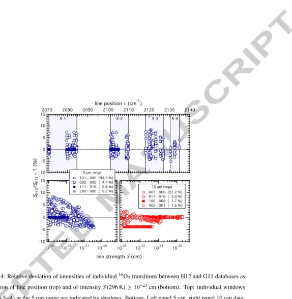
Figure 4: Relative deviation of intensities of individual16O
3transitions between H12 and G11 databases as
a function of line position (top) and of intensity S (296 K)≥ 10−23cm (bottom). Top: individual windows (5−1 to 5−4) in the 5 µm range are indicated by shadows. Bottom: Left panel 5 µm, right panel 10 µm data. Line data common to the two databases and corresponding to the four most intense bands (with weights given in the legends) are shown.
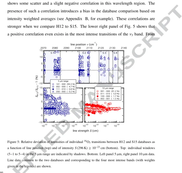
shows some scatter and a slight negative correlation in this wavelength region. The presence of such a correlation introduces a bias in the database comparison based on intensity weighted averages (see Appendix B, for example). These correlations are stronger when we compare H12 to S15. The lower right panel of Fig. 5 shows that a positive correlation even exists in the most intense transitions of theν3band. From
Figure 5: Relative deviation of intensities of individual16O
3transitions between H12 and S15 databases as
a function of line position (top) and of intensity S (296 K)≥ 10−23cm (bottom). Top: individual windows (5−1 to 5−4) in the 5 µm range are indicated by shadows. Bottom: Left panel 5 µm, right panel 10 µm data. Line data common to the two databases and corresponding to the four most intense bands (with weights given in the legends) are shown.
365
a linear fit of∆S/S vs. S (235 K) in the range S > 10−21cm on transitions in theν3
band of the main isotope, we derive a slope of+3.6 · 1017cm−1and inspection of the
H12 database shows that 2[E(S3)/E(S2)− E(S2)/E(S )] = 7.9 · 10−21cm (for further
details see Appendix B). According to eq. (B.6), this results in an overrestimation of the adjusted intensities by about 0.3 %. Ozone columns will thus be underestimated by
370
the same relative amount, when adjusted intensity values are used and this corresponds exactly to the observed difference between retrievals based on S15 and H12 displayed in Fig. 3.
4.2. 5 µm region
Figure 6: Total ozone column densitiesCO3from the 5 µm windows 5−1 to 5−4 as relative deviation with
respect to the retrieval from the 10 µm window (10−1). Panels from left to right show results for the H12, G11 and S15 database, respectively. Individual 5 µm windows are indicated by symbol shades.
Column densities from the 5 µm windows are represented in Fig. 6 as relative
devia-375
tion from the result in the 10 µm window. Independent of the database, the results from the two wavelength regions are coherent to better than±3 %. Averages over individual windows are within−1.0 and +1.6 % for H12, within −1.0 and −2.3 % for G11 and within−0.3 and +0.5 % for S15. While G11 data thus give a consistent negative offset of about (−1.9 ± 0.6) % (1 σ dispersion of window averages) with little dispersion and
380
while S15 has an insignificant offset with an even smaller dispersion of (0.2 ± 0.4) %, the H12 data have a positive offset of (1.4 ± 0.4) % for windows 5−2 through 5−4. The 5−1 window, which is dominated by transitions belonging to the P-branch of the ν1+ ν3 band, however is not consistent with this positive shift and shows an offset of
−1.0 %. Note that the dispersion within each window (1 σ, N = 93) is in the 0.3 to
385
0.4 % range. This single intra-window dispersion is independent of the window and the database used and thus mereley reflects measurement uncertainties.
We point out that our atmospherically observed offset of +1.4 % between 5 and 10 µm regions when using H12 is in full agreement with a recent laboratory study [27]. The laboratory derived intensities deviate from H12 by (−1.96 ± 0.29) and
390
(−0.34±0.11) % at 5 and 10 µm, respectively. This implies CH12
O3 (5 µm)/C H12
O3 (10 µm)=
tistically derived uncertainty of the individual averages at 5 and 10 µm. The compar-ison with this measurement and the fact that line-mixing does not measurably change total ozone columns from the 5 µm range under atmospheric conditions [52, see
Ta-395
ble 1], let us conclude that line-mixing impacts total ozone columns from the 10 µm region (window 10−1) by an amount less than the dispersion of our measurements. A similar conclusion must be drawn from the comparison with the slightly higher value CH12
O3 (5 µm)/C H12
O3 (10 µm) = (+2.1 ± 0.3) % derived in another laboratory study
un-der high pressure conditions (0.3 − 1 bar), where line-mixing effects have been taken
400
into account in the analysis [52]. This high degree of agreement with both laboratory experiments implies that the effect of line-mixing on the derived total ozone column densities is small and likely less than about 0.7 %. The full agreement between re-trieval results from all windows within the scatter of about 0.4 % when S15 is used (right panel of Fig. 6) indeed provides very strong support for line-mixing effects
ac-405
tually being smaller than 0.4 %. Anyway, they are smaller than most of the effects that we are about to discuss in the following.
The differences of about 3.5 % (windows 5−2 through 5−4) between the G11 and H12 databases can be easily understood on the background of our previous analysis and discussion concerning the 10 µm region. Calculation of intensity weighted spectral
410
parameters at 235 K shows that in each of the windows most of the absorbed intensity is due to the 101← 000 band. This band has a roughly 3 (5−1) to 4 % (5−2 to 5−4) higher weighted intensity in G11 than in H12 (see Table 6), implying that the column densities must be correspondingly lower. From this∼ 4 % correction, the 0.6 % difference in the 10 µm region must be subtracted. The resulting shift inCO3(5 µm)/CO3(10 µm) 415
of 3.4 % is fully consistent with the atmospheric observation in Fig. 6. We note that intensities of these overtone and combination bands are sufficiently weak for non-linear absorption effects, such as observed in the ν3 fundamental at 10 µm, being of little
importance.
Table 6 further shows that the ratio of ozone columns derived from the two databases
420
at 5 µmCH12
O3 (5 µm)/C G11
O3 (5 µm) cannot be consistent over all windows at the accuracy
level of 1 %. The weighted average analysis confirms that the column ratioCH12 O3 (5 µm)
/ CG11
G11 database are consistent over all four windows, we suspect that the problem is linked to the spectroscopic data in H12. However, the simplified database comparison
425
in Table 6 gives a difference of only 1.4 % and rests below the observed discrepancy of about 2 to 2.5 %. These database differences are further corroborated by the excellent agreement found in the S15 based retrievals.
As an aside we note here that the 111← 010 hot band has identical intensity entries in all three different databases. This becomes evident from Fig. 5, but is also reflected
430
in the corresponding entries in Table 6, which are all identical zero.
The large intensity dependent differences in line strengths of 2ν1, 2ν3andν1+ ν3
band transitions between the G11 and H12 databases (see left panel of Fig. 4) prevent intensity weighted averages to be used for globally rescaling one database with respect to the other in order to resolve observed discrepancies in the 5 µm region. The
col-435
umn biases associated with a weighted intensity correction, that are obtained from the procedure described in section 4.1 are around 1.4 %. It thus seems that this particular spectral region requires new experimental and theoretical studies to be undertaken. The high consistency of the S15 based retrievals possibly indicates that the S&MPO (S15) database presently is the most adequate to use for retrieving ozone from the 5 and 10
440
µm regions, and that the underlying data and spectroscopic analysis already provide the desired level of accuracy of better than 1 %. But so far these data have not been published in the literature. It must also be kept in mind that our study cannot assess the absolute accuracy of the spectroscopic data and since our observations are based on lines from very restricted spectral ranges (see Fig. 1), little can be said about data
445
quality concerning transitions outside the observational windows.
5. Conclusion and Outlook
We have compared ozone spectroscopic data in the 5 and 10 µm spectral regions from different databases and confronted them with ground based atmospheric spectra, acquired with the high-resolution FTS-Paris instrument. In order to clearly attribute
450
differences in retrieved ozone columns to differences in the spectroscopic databases, we have also performed direct database comparisons restricted to the observational
windows, using intensity weighted averages of the chief spectroscopic parameters. Using the atmospheric spectra, a complete sensitivity analysis of the four spectro-scopic parameters intensity (S ), air-broadening half width (γair), its temperature
coef-455
ficient (nair) and the lower state energy (E′′) has been performed in the 10 µm region.
Relative uncertainties of these parameters belonging to transitions in theν3
fundamen-tal band impact on the tofundamen-tal ozone columns with respective of weights−1 : −0.15 : −0.05 , for S , γair and nair. For transitions belonging to weaker bands in the same
region, sensitivity coefficients for S , γair and nair scale as−1 : +0.29 : +0.055. The
460
observed sensitivity coefficients have been confirmed by theoretical analysis and nu-merical simulations. Current database uncertainties in E′′ do not affect retrievals and can be neglected. The derived sensitivity coefficients might guide further studies that aim at improving on the uncertainty of total ozone column retrievals in that region.
The three databases HITRAN, GEISA and S&MPO have been characterized with
465
respect to their utility for atmospheric retrievals. Using the spectroscopic data in the 991.25 − 1013.19 cm-1 window range, total ozone column retrievals with the three databases gave results that agreed to clearly better than 1 %. Much of the difference is due to slight differences in the spectroscopic data and, in case of in the GEISA database, the lack of17O-containing ozone. This degree of agreement is confirmed by 470
direct comparison of spectroscopic databases, using intensity weighted averages of the spectroscopic parameters.
Deviations between the databases in the 5 µm region are larger, however. Ozone columns derived in that wavelength range differ by about 4 %, which is likely due to a global adjustment of line intensities [18] in the HITRAN database in 2004, which
475
has only partially been adopted in the GEISA database. Nevertheless, each of the three databases gives total ozone columns at 5 µm that generally agree within±2 % with the results obtained at 10 µm. Retrievals using the S&MPO data show an even better agreement within less than±1 %, both between the 5 and 10 µm regions and within the 5 µm region itself.
480
Importantly, all four windows in the 5 µm region yield consistent ozone columns when we use parameters from the GEISA or S&MPO databases. This is not the case when parameters are taken from HITRAN. Employing HITRAN parameters, one of
the windows (2070.90 − 2084.64 cm-1), mostly containing P-branch transitions from
theν1+ ν3combination band in the 5 µm region results in ozone columns that are sig-485
nificantly lower (1.5 − 3.0 %) than the ones obtained from the other three windows. This striking difference between databases is corroborated by direct comparison of the intensity weighted average intensities in the four windows. While average intensities between HITRAN and GEISA databases differ by 4.1 % in the three coherent windows, they differ by only 2.7 % in the particular window between 2070.90 and 2084.64 cm-1. 490
The inferred difference of 1.4 % is close to the observed discrepancy, which thus con-firms that the observed mismatch is due to the ozone spectroscopic data in the two databases and not linked to the measurement process or the retrieval procedure. This fact is further corroborated by the excellent consistency of results when either GEISA or S&MPO are used for the retrieval.
495
While the comparison in the 10 µm region has shown that all databases yield very consistent results at a high level of precision (< 1 %), the detailed analysis of the 5 µm region shows that a similar precision level has not yet been reached there. Only the S&MPO database gives entirely consistent results at the 1 % level. Thus, further lab-oratory studies targetting at the 5 µm and other spectral regions are required. So are
500
new theoretical calculations [10] and validation procedures for incorporating new line parameter data into the databases.
With the availability of more and more spectroscopic databases or linelists, the simple method of comparing intensity weighted spectroscopic parameter averages may provide an interesting tool for analyzing these databases for consistency and thus for
505
identifying critical regions for remote sensing applications. While the approach avoids entering into the tedious work of analyzing individual transitions, it remains to be shown that its application is useful for the remote sensing of molecules other than ozone.
Appendix A. Sensitivity
510
Appendix A.1. Band specific sensitivity coefficients and intensity weights
In this appendix, definitions for the band specific sensitivity coefficients and inten-sity weights are given. We first define the band specific sensitivity coefficient αI(x)
αI(x)= 1 wI ( ∆CO3 CO3 )/ ( ∆xI xI ) (A.1)
where xI indicates that parameter changes of a rovibrational transition are considered
only if this transition belongs to the particular band I. The weight wI of the vibrational
515
band I is the defined as the ratio of the pseudo band intensity ˆSI over the integrated
intensity of all rovibrational transitions within the considered window M:
wI = ˆSI
/ ∑
j∈M
Sj, (A.2)
where the Sj are line strengths of individual rovibrational transitions j. The pseudo
band intensity ˆSIcorresponds to the total band intensity restricted to transitions within
the observational window M, i.e.:
520 ˆ SI = ∑ j∈I ∧ j∈M Sj. (A.3)
Appendix A.2. Simulation of pressure braodening
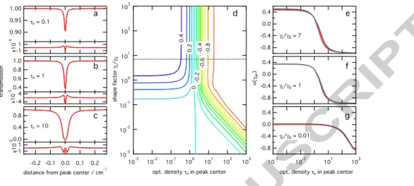
We assume a Voigt line shape for a molecular transition and simulate molecular absorption in a homogeneous atmosphere. Three parameters are required: the Gaussian (Doppler) width which is described by the HWHM parameterγG, the Lorentzian width
for the pressure broadening, given by the HWHM parameterγL = γair × p, and the
525
optical density at peak centerτ0. In the atmospheric retrieval, widths are determined by
temperature and pressure conditions and the corresponding values therefore are fixed in the fitting process. Nevertheless, the Lorentzian width may be off by a bias in γair. This
effect is investigated through fitting a Voigt line profile with a small bias in γL(1.02
times the width of the original profile), leading to a non-zero residual and a biased
530
value for the peak area. The results of these simulations are shown in Figures A.7a-c, where transmission curves of the absorption lines and the fit residuals are displayed
for different optical densities τ0. As can be seen, the residuals change from a V to a
W-shape when increasingτ0from 0.1 to 10. For the simulation, the Doppler width has
been fixed to a typical value ofγG= 0.1 cm-1, but the result is completely independent
535
of the exact value used. It only depends on the shape parameterβ (eq. (4)), which was fixed toβ = 7 in Figs. A.7 a-c for matching typical atmospheric conditions.
In Figure A.7 d, a simulated value ofα(γair) has been calculated by equation (5),
using∆x/x = 0.02 for various combinations of τ0andβ. In the high pressure limit (β ≥
10),α(γair) becomes independent of the shape parameter. This is expected, because the
540
width is dominated by pressure broadening anyway and a bias in this parameter should have its maximum effect. In the low pressure limit (β ≤ 0.1), one expects that biases in γLcan be neglected, because the line shape is dominated by Doppler broadening. For
weak absorptionsτ0< 1, α(γair) is indeed about 0. At large optical densities however,
α(γair) never vanishes because the wings of the Lorentzian have still an impact on the fit
545
far from the line center, even though the HWHM width is completely dominated by the Doppler profile. This wing effect scales linearly with τ0and the asymptotical behavior
ofα(γair) is given by the productτ0×β = const. Figures A.7e-g then illustrate for fixed
values ofβ how α(γair) varies as a function of the optical density. At high pressures
(β = 7), it changes from about +0.45 to −1 at τ0 ∼ 100 (Fig. A.7e). At low pressures, 550
the low optical density limit approaches zero and the transition towards negative values shifts towards higher peak absorption values.
These results onα(γair) are robust and do only weakly depend on the exact
knowl-edge ofγair: Comparing the fit results of two line profiles biased by 12 and 10 % inγair,
respectively, gave a similar difference in retrieved intensities than comparing a line with
555
2 % bias to the unbiased line. Grey curves in Figures A.7e-g show the results derived from biases offset by ±10 %, which is deemed a reasonable range for the uncertainty of the published data. Because it is independent on pressure in theβ ≥ 7 range which is characteristic for most of the vertical ozone distribution (see section 3.1),α(γair)
should follow theτ0dependency given in Figure A.7e. 560
Figure A.7: Sensitivity of the column on biases in theγairparameter from a simple numerical simulation.
Panels a through c show Voigt profiles and fit residuals, whenγairis biased by+2% for peak center optical
densitiesτ0of 0.1, 1, and 10, respectively. The Gaussian HWHM, and the shape parameter have respectively
been fixed to characteristic value ofγG= 0.1 cm-1andβ = γL/γG = 7. Panel d shows α(γair) as a function
of the peak absorptionτ0and the shape parameterγL/γG. Contour lines are separated by units of 0.1 and
the dashed horizontal line indicatesβ = 7. Panels e to g then display α(γair) as a function of the peak
optical densityτ0forβ fixed to values of 7, 1, and 0.01 (red lines). Grey lines indicate in as much the bias
ofα(γair) depends on the absolute valueγair. Shaded regions in panels e-g indicate estimated atmospheric
absorption conditions for the asymmetric stretch (ν3) withτ0 ≃ 9 on the one hand and the weaker bands
(0.08 ≤ τ0≤ 0.6) on the other hand.
Appendix B. Bias of intensity weighted averages
We have introduced intensity weighted averages as a practical means of direct comparison of spectroscopic parameters in different databases, which introduces an effective cutoff of weak absorption lines. Here we show that correcting values in one database by the ratio of averages between the two databases does not necessarily
repro-565
duce the results of the latter in an atmospheric retrieval and thus introduces a bias. This depends on whether the spectroscopic data correlate with the line intensities or not.
We start from the idealizing assumption that each line contributes to the retrieved absorption signal proportional to its line intensity (ie we neglect the presence of noise in the atmospheric measurement). The expectation value or mean E of the statistic of
intensities S is defined by E(S )= 1 N N ∑ i=1 Si. (B.1)
For what follows, we recall that the second and third moments of S are similarly de-fined as E(S2) and E(S3), respectively. Like E(S ), these quantities can be easily cal-culated from the data given in the spectroscopic databases. We assume that the values in the two databases SHand SGsuffer from small biases with respect to the true distri-575
bution of intensity values S :
SH= (1 + a + bS )S (B.2)
SG= (1 + c + dS )S (B.3)
The coefficients a and c denote relative offsets of the database values with respect to the true values and coefficients b and d , 0 indicate a linear correlation of the bias with intensity. In this case the ratio R of expectation values is given by
R = E(SH) E(SG) =E((1+ a + bS )S ) E((1+ c + dS )S ) ≃ 1+ a 1+ c 1 + (b − d)E ( S2) E(S ) , (B.4)
where the last transformation holds to the degree that terms of second order in the supposedly small deviations a, b, c and d can be neglected. Due to the ratio of weighted averages Ew(eqs. (A.3) and (A.2)) being
Rw= Ew(SH) Ew(SG) = R−1E(S2H) E(S2 G) , (B.5) we find that 580 Rw/R = R−2 E(S2 H) E(S2 G) ≃ 1 + 2(b − d) ( E(S3) E(S2)− E(S2) E(S ) ) , (B.6)
where in the last step we have once again neglected higher than linear order terms in a, b, c and d. Our bias is thus given by the second term in equation (B.6). Evidently, only if b, d, we introduce a bias by comparing intensity weighted averages. Note that if
b= d = 0, the approximations in eqs. (B.4) and (B.6) become exact and any constant relative offset between the two databases is inferred without any bias.
585
A non-zero term (b− d) might be inferred as the slope of the linear fit on the ∆S/S over S data, such as in Fig. 4 and the expression in parantheses can be simply estimated from using either SHor SGfor the unknown S . In this way the bias can be determined
and accounted for.
Acknowledgement
590
This work was supported by the french national programme LEFE/INSU. The authors would like to express their gratitude for the valuable technical support of H. Elandaloussi, P. Marie-Jeanne, and C. Rouill´e.
References
[1] J. Viallon, P. Moussay, J. E. Norris, F. R. Guenther, R. I. Wielgosz, Metrologia 43
595
(2006) 441–450.
[2] P. J. Nair, S. Godin-Beekmann, J. Kuttippurath, G. Ancellet, F. Goutail, A. Pazmino, L. Froidevaux, J. M. Zawodny, R. D. Evans, H. J. Wang, Atmos. Chem. Phys. 13 (2013) 10373–10384.
[3] S. B. Andersen, E. C. Weatherhead, A. Stevermer, J. Austin, C. Br¨uhl, E. L.
600
Fleming, J. de Grandpr´e, V. Grewe, I. Isaksen, G. Pitari, J. Geophys. Res. Atmos. 111 (2006).
[4] C. Vigouroux, T. Blumenstock, M. Coffey, Q. Errera, O. Garc´ıa, N. B. Jones, J. W. Hannigan, F. Hase, B. Liley, E. Mahieu, J. Mellqvist, J. Notholt, M. Palm, G. Persson, M. Schneider, C. Servais, D. Smale, L. Th¨olix, M. De Mazi`ere,
At-605
mos. Chem. Phys. 15 (2015) 2915–2933.
[5] A. Tandon, A. K. Attri, Atmos. Environ. 45 (2011) 1648–1654.
[6] C. Janssen, D. Simone, M. Guinet, Rev. Sci. Instr. 82 (2011) 034102. doi:10. 1063/1.3557512.
[7] M. Petersen, J. Viallon, P. Moussay, R. I. Wielgosz, J. Geophys. Res. 117 (2012).
610
[8] J. Viallon, S. Lee, P. Moussay, K. Tworek, M. Petersen, R. I. Wielgosz, Atmos. Meas. Tech. 8 (2015) 1245–1257.
[9] J. M. Flaud, R. Bacis, Spectrochim. Acta A 54 (1998) 3–16.
[10] A. Barbe, S. Mikhailenko, E. Starikova, M. R. De Backer, V. Tyuterev, D. Monde-lain, S. Kassi, A. Campargue, C. Janssen, S. Tashkun, J. Quant. Spectrosc. Radiat.
615
Trans. 130 (2013) 172–190.
[11] B. Hassler, I. Petropavlovskikh, J. Staehelin, T. August, P. K. Bhartia, C. Cler-baux, D. Degenstein, M. D. Mazi`ere, B. M. Dinelli, A. Dudhia, G. Dufour, S. M. Frith, L. Froidevaux, S. Godin-Beekmann, J. Granville, N. R. P. Harris, K. Hop-pel, D. Hubert, Y. Kasai, M. J. Kurylo, E. Kyr¨ol¨a, J. C. Lambert, P. F. Levelt, C. T.
620
McElroy, R. D. McPeters, R. Munro, H. Nakajima, A. Parrish, P. Raspollini, E. E. Remsberg, K. H. Rosenlof, A. Rozanov, T. Sano, Y. Sasano, M. Shiotani, H. G. J. Smit, G. Stiller, J. Tamminen, D. W. Tarasick, J. Urban, R. J. van der A, J. P. Veefkind, C. Vigouroux, T. von Clarmann, C. von Savigny, K. A. Walker, M. We-ber, J. Wild, J. M. Zawodny, Atmos. Meas. Tech. 7 (2014) 1395–1427.
625
[12] M. A. H. Smith, V. M. Devi, D. C. Benner, C. P. Rinsland, J. Geophys. Res. 106 (2001) 9909–9921.
[13] C. Claveau, C. Camy-Peyret, A. Valentin, J. M. Flaud, J. Molec. Spectrosc. 206 (2001) 115–125.
[14] G. Wagner, M. Birk, F. Schreier, J. M. Flaud, J. Geophys. Res. 107 (2002) 4626.
630
doi:10.1029/2001JD000818.
[15] M. R. DeBacker-Barilly, A. Barbe, J. Molec. Spectrosc. 205 (2001) 43–53.
[16] J. M. Flaud, G. Wagner, M. Birk, C. Camy-Peyret, C. Claveau, M. R. DeBacker-Barilly, A. Barbe, C. Piccolo, J. Geophys. Res. 108 (2003). doi:10.1029/ 2002JD002755.
[17] N. Jacquinet-Husson, N. Scott, A. Chedin, K. Garceran, R. Armante, A. Chursin, A. Barbe, M. Birk, L. Brown, C. Camy-Peyret, C. Claveau, C. Clerbaux, P. Co-heur, V. Dana, L. Daumont, M. Debacker-Barilly, J. Flaud, A. Goldman, A. Ham-douni, M. Hess, D. Jacquemart, P. Kopke, J. Mandin, S. Massie, S. Mikhailenko, V. Nemtchinov, A. Nikitin, D. Newnham, A. Perrin, V. Perevalov, L.
Regalia-640
Jarlot, A. Rublev, F. Schreier, I. Schult, K. Smith, S. Tashkun, J. Teffo, R. Toth, V. Tyuterev, J. Auwera, P. Varanasi, G. Wagner, J. Quant. Spectroscop. Radiat. Transfer 95 (2005) 429–467.
[18] L. S. Rothman, D. Jacquemart, A. Barbe, D. C. Benner, M. Birk, L. R. Brown, M. R. Carleer, C. Chackerian, Jr, K. Chance, L. H. Coudert, V. Dana, V. M. Devi,
645
J.-M. Flaud, R. R. Gamache, A. Goldman, J.-M. Hartmann, K. W. Jucks, A. G. Maki, J.-Y. Mandin, S. T. Massie, J. Orphal, A. Perrin, C. P. Rinsland, M. A. H. Smith, J. Tennyson, R. N. Tolchenov, R. A. Toth, J. Vander Auwera, P. Varanasi, G. Wagner, J. Quant. Spectrosc. Radiat. Trans. 96 (2005) 139 – 204.
[19] L. S. Rothman, I. E. Gordon, A. Barbe, D. C. Benner, P. F. Bernath, M. Birk,
650
V. Boudon, L. R. Brown, A. Campargue, J. P. Champion, K. Chance, L. H. Coud-ert, V. Dana, V. M. Devi, S. Fally, J. M. Flaud, R. R. Gamache, A. Goldman, D. Jacquemart, I. Kleiner, N. Lacome, W. J. Lafferty, J. Y. Mandin, S. T. Massie, S. N. Mikhailenko, C. E. Miller, N. Moazzen-Ahmadi, O. V. Naumenko, A. V. Nikitin, J. Orphal, V. I. Perevalov, A. Perrin, A. Predoi-Cross, C. P. Rinsland,
655
M. Rotger, M. Simeckov´a, M. A. H. Smith, K. Sung, S. A. Tashkun, J. Tennyson, R. A. Toth, A. C. Vandaele, J. Vander Auwera, J. Quant. Spectrosc. Radiat. Trans. 110 (2009) 533–572.
[20] A. Gratien, B. Picquet-Varrault, J. Orphal, J. F. Doussin, J. M. Flaud, J. Phys. Chem. A 114 (2010) 10045–10048. doi:10.1021/jp103992f.
660
[21] B. Picquet-Varrault, J. Orphal, J.-F. Doussin, P. Carlier, J.-M. Flaud, J. Phys. Chem. A 109 (2005) 1008 – 1014. doi:10.1021/jp0405411.
Flaud, T. Blumenstock, J. Orphal, Atmos. Meas. Tech. 4 (2011) 535–546. doi:10. 5194/amt-4-535-2011.
665
[23] E. Dupuy, K. A. Walker, J. Kar, C. D. Boone, C. T. McElroy, P. F. Bernath, J. R. Drummond, R. Skelton, S. D. McLeod, R. C. Hughes, C. R. Nowlan, D. G. Du-four, J. Zou, F. Nichitiu, K. Strong, P. Baron, R. M. Bevilacqua, T. Blumen-stock, G. E. Bodeker, T. Borsdorff, A. E. Bourassa, H. Bovensmann, I. S. Boyd, A. Bracher, C. Brogniez, J. P. Burrows, V. Catoire, S. Ceccherini, S. Chabrillat,
670
T. Christensen, M. T. Coffey, U. Cortesi, J. Davies, C. De Clercq, D. A. Degen-stein, M. De Mazi`ere, P. Demoulin, J. Dodion, B. Firanski, H. Fischer, G. Forbes, L. Froidevaux, D. Fussen, P. Gerard, S. Godin-Beekmann, F. Goutail, J. Granville, D. Griffith, C. S. Haley, J. W. Hannigan, M. H¨opfner, J. J. Jin, A. Jones, N. B. Jones, K. Jucks, A. Kagawa, Y. Kasai, T. E. Kerzenmacher, A. Kleinb¨ohl, A. R.
675
Klekociuk, I. Kramer, H. K¨ullmann, J. Kuttippurath, E. Kyr¨ol¨a, J.-C. Lambert, N. J. Livesey, E. J. Llewellyn, N. D. Lloyd, E. Mahieu, G. L. Manney, B. T. Mar-shall, J. C. McConnell, M. P. McCormick, I. S. McDermid, M. McHugh, C. A. McLinden, J. Mellqvist, K. Mizutani, Y. Murayama, D. P. Murtagh, H. Oelhaf, A. Parrish, S. V. Petelina, C. Piccolo, J.-P. Pommereau, C. E. Randall, C. Robert,
680
C. Roth, M. Schneider, C. Senten, T. Steck, A. Strandberg, K. B. Strawbridge, R. Sussmann, D. P. J. Swart, D. W. Tarasick, J. R. Taylor, C. T´etard, L. W. Thoma-son, A. M. ThompThoma-son, M. B. Tully, J. Urban, F. Vanhellemont, C. Vigouroux, T. von Clarmann, P. von der Gathen, C. von Savigny, J. W. Waters, J. C. Witte, M. Wolff, J. M. Zawodny, Atmos. Chem. Phys. 9 (2009) 287–343.
685
[24] L. S. Rothman, A. Barbe, D. Chris Benner, L. R. Brown, C. Camy-Peyret, M. R. Carleer, K. Chance, C. Clerbaux, V. Dana, V. M. Devi, A. Fayt, J. M. Flaud, R. R. Gamache, A. Goldman, D. Jacquemart, K. W. Jucks, W. J. Lafferty, J. Y. Mandin, S. T. Massie, V. Nemtchinov, D. A. Newnham, A. Perrin, C. P. Rinsland, J. Schroeder, K. Smith, M. A. H. Smith, K. Tang, R. A. Toth, J. Vander Auwera,
690
P. Varanasi, K. Yoshino, J. Quant. Spectroscop. Radiat. Trans. 82 (2003) 5–44.
[25] M. Guinet, D. Mondelain, C. Janssen, C. Camy-Peyret, J. Quant. Spectrosc. Ra-diat. Trans. 111 (2010) 961–972.
[26] D. G. Dufour, J. R. Drummond, C. T. McElroy, C. Midwinter, P. F. Bernath, K. A. Walker, W. F. J. Evans, E. Puckrin, C. Nowlan, J. Phys. Chem. A 109 (2005)
695
8760–8764.
[27] X. Thomas, P. Von Der Heyden, M. R. De Backer-Barilly, M. T. Bourgeois, A. Barbe, J. Quant. Spectrosc. Radiat. Trans. 111 (2010) 1080–1088. doi:10. 1016/j.jqsrt.2010.02.001.
[28] K. A. Walker, C. Boone, R. Skelton, S. D. McLeod, P. F. Bernath, C. E. Randall,
700
C. R. Trepte, K. Strong, T. C. McElroy, in: ENVISAT Symposium April 2007, Montreux (Switzerland).
[29] O. E. Garc´ıa, M. Schneider, F. Hase, T. Blumenstock, E. Sepulveda, Y. Gonz´alez, Atmos. Meas. Tech. 7 (2014) 3071–3084.
[30] M. Schneider, F. Hase, J. Quant. Spectroscop. Radiat. Trans. 110 (2009) 1825–
705
1839.
[31] N. Jacquinet-Husson, L. Crepeau, R. Armante, C. Boutammine, A. Chedin, N. Scott, C. Crevoisier, V. Capelle, C. Boone, N. Poulet-Crovisier, A. Barbe, A. Campargue, D. Chris Benner, Y. Benilan, B. B´ezard, V. Boudon, L. R. Brown, L. H. Coudert, A. Coustenis, V. Dana, V. M. Devi, S. Fally, A. Fayt,
710
J. M. Flaud, A. Goldman, M. Herman, G. Harris, D. Jacquemart, A. Jolly, I. Kleiner, A. Kleinb¨ohl, F. Kwabia-Tchana, N. Lavrentieva, N. Lacome, L.-H. Xu, O. Lyulin, J. Y. Mandin, A. Maki, S. Mikhailenko, C. E. Miller, T. Mishina, N. Moazzen-Ahmadi, H. M¨uller, A. Nikitin, J. Orphal, V. Perevalov, A. Perrin, D. Petkie, A. Predoi-Cross, C. P. Rinsland, J. Remedios, M. Rotger, M. A. H.
715
Smith, K. Sung, S. Tashkun, J. Tennyson, R. A. Toth, A. C. Vandaele, J. Van-der Auwera, J. Quant. Spectroscop. Radiat. Trans. 112 (2011) 2395–2445.
[32] L. S. Rothman, I. E. Gordon, Y. Babikov, A. Barbe, D. Chris Benner, P. F. Bernath, M. Birk, L. Bizzocchi, V. Boudon, L. R. Brown, A. Campargue, K. Chance, E. A. Cohen, L. H. Coudert, V. M. Devi, B. J. Drouin, A. Fayt, J. M. Flaud,
720
R. R. Gamache, J. J. Harrison, J. M. Hartmann, C. Hill, J. T. Hodges, D. Jacque-mart, A. Jolly, J. Lamouroux, R. J. Le Roy, G. Li, D. A. Long, O. M. Lyulin,
C. J. Mackie, S. T. Massie, S. Mikhailenko, H. S. P. M¨uller, O. V. Naumenko, A. V. Nikitin, J. Orphal, V. Perevalov, A. Perrin, E. R. Polovtseva, C. Richard, M. A. H. Smith, E. Starikova, K. Sung, S. Tashkun, J. Tennyson, G. C. Toon,
725
V. G. Tyuterev, G. Wagner, J. Quant. Spectrosc. Radiat. Trans. 130 (2013) 4–50.
[33] Y. L. Babikov, S. N. Mikhailenko, A. Barbe, V. G. Tyuterev, J. Quant. Spectro-scop. Radiat. Trans. 145 (2014) 169–196.
[34] Y. T´e, P. Jeseck, S. Payan, I. Pepin, C. Camy-Peyret, Rev. Sci. Instr. 81 (2010) 103102.
730
[35] L. S. Rothman, C. P. Rinsland, A. Goldman, S. T. Massie, D. P. Edwards, J. M. Flaud, A. Perrin, C. Camy-Peyret, V. Dana, J. Y. Mandin, J. Schroeder, A. Mc-Cann, R. R. Gamache, R. B. Wattson, K. Yoshino, K. V. Chance, K. W. Jucks, L. R. Brown, V. Nemtchinov, P. Varanasi, J. Quant. Spectroscop. Radiat. Trans. 60 (1998) 665–710.
735
[36] T. B. Coplen, J. K. B¨ohlke, P. De Bi`evre, T. Ding, N. E. Holden, J. A. Hopple, H. R. Krouse, A. Lamberty, H. S. Peiser, K. R´ev´esz, S. E. Rieder, K. J. R. Rosman, E. Roth, P. D. P. Taylor, R. D. Vocke, Y. K. Xiao, Pure Appl. Chem. 74 (2002) 1987–2017.
[37] C. A. M. Brenninkmeijer, C. Janssen, J. Kaiser, T. R¨ockmann, T. S. Rhee, S. S.
740
Assonov, Chem. Rev. 103 (2003) 5125–5161.
[38] D. Krankowsky, P. L¨ammerzahl, K. Mauersberger, C. Janssen, B. Tuzson, T. R¨ockmann, J. Geophys. Res. 112 (2007) D08301.
[39] A. M. Goldman, F. J. Murcray, D. G. Murcray, J. J. Kosters, C. P. Rinsland, J. M. Flaud, C. Camy-Peyret, A. Barbe, J. Geophys. Res. 94 (1989) 8467–8473.
745
[40] J.-M. Flaud, C. Piccolo, P. Cali, A. Perrin, L. H. Coudert, J.-L. Teffo, L. R. Brown, Atmos. Oceanic Opt. 16 (2003) 172 – 182.
[41] J. Flaud, C. Camy-Peyret, C. P. Rinsland, M. A. H. Smith, V. M. Devi, Atlas of ozone spectral parameters from microwave to medium infrared, Academic Press Inc., Boston, 1990.
[42] A. Barbe, J. J. Plateaux, S. Bouazza, O. Sulakshina, S. Mikhailenko, V. Tyuterev, S. Tashkun, J. Quant. Spectroscop. Radiat. Transfer 52 (1994) 341–355.
[43] A. Barbe, V. G. Tyuterev, 2013. Pers. communication.
[44] F. Hase, J. W. Hannigan, M. T. Coffey, A. Goldman, M. Hopfner, N. B. Jones, C. P. Rinsland, S. W. Wood, J. Quant. Spectroscop. Radiat. Trans. 87 (2004) 25–
755
52.
[45] S. A. Clough, M. W. Shephard, E. J. Mlawer, J. S. Delamere, M. J. Iacono, K. Cady-Pereira, S. Boukabara, P. D. Brown, J. Quant. Spectroscop. Radiat. Trans. 91 (2005) 233–244.
[46] F. Hase, Atmos. Meas. Tech. 5 (2012) 603–610.
760
[47] F. Hase, T. Blumenstock, C. Paton-Walsh, Appl. Opt. 38 (1999) 417–3422.
[48] M. Schneider, F. Hase, Atmos. Chem. Phys. 8 (2008) 63–71.
[49] A. Laeng, U. Grabowski, T. von Clarmann, G. Stiller, N. Glatthor, M. Hopfner, S. Kellmann, M. Kiefer, A. Linden, S. Lossow, Atmos. Meas. Tech. 7 (2014) 3971–3987.
765
[50] R. Lindenmaier, R. L. Batchelor, K. Strong, H. Fast, F. Goutail, F. Kolonjari, C. T. McElroy, R. L. Mittermeier, K. A. Walker, J. Quant. Spectroscop. Radiat. Transfer 111 (2009) 569–585.
[51] H. Tran, F. Rohart, C. Boone, M. Eremenko, F. Hase, P. Bernath, J. M. Hart-mann, J. Quant. Spectrosc. Radiat. Trans. 111 (2010) 2012–2020. doi:10.1016/
770
j.jqsrt.2010.04.002.
[52] H. Tran, B. Picquet-Varrault, C. Boursier, C. Viatte, M. Eremenko, F. Hase, J. M. Hartmann, J. Quant. Spectrosc. Radiat. Trans. 112 (2011) 2287–2295. doi:10. 1016/j.jqsrt.2011.06.001.