HAL Id: hal-00299357
https://hal.archives-ouvertes.fr/hal-00299357
Submitted on 27 Jul 2006
HAL is a multi-disciplinary open access
archive for the deposit and dissemination of
sci-entific research documents, whether they are
pub-lished or not. The documents may come from
teaching and research institutions in France or
abroad, or from public or private research centers.
L’archive ouverte pluridisciplinaire HAL, est
destinée au dépôt et à la diffusion de documents
scientifiques de niveau recherche, publiés ou non,
émanant des établissements d’enseignement et de
recherche français ou étrangers, des laboratoires
publics ou privés.
combined clutter and beam blockage correction
technique
A. Fornasiero, J. Bech, P. P. Alberoni
To cite this version:
A. Fornasiero, J. Bech, P. P. Alberoni. Enhanced radar precipitation estimates using a combined
clut-ter and beam blockage correction technique. Natural Hazards and Earth System Science, Copernicus
Publications on behalf of the European Geosciences Union, 2006, 6 (5), pp.697-710. �hal-00299357�
© Author(s) 2006. This work is licensed under a Creative Commons License.
and Earth
System Sciences
Enhanced radar precipitation estimates using a combined clutter
and beam blockage correction technique
A. Fornasiero1,2, J. Bech3,4, and P. P. Alberoni1
1Servizio IdroMeteorologico, A.R.P.A. Emilia Romagna, Viale Silvani, 6, 40122 Bologna, Italy
2Centro di ricerca Interuniversitario in Monitoraggio Ambientale, Polo Accademico Savonese, Via Cadorna 7, 17100 Savona, Italy
3Servei Meteorol`ogic de Catalunya, Berlin 38, 08029 Barcelona, Spain
4Dep. d’Astronomia i Meteorologia, Universitat de Barcelona, Mart´ı i Franqu´es, 1, 08028 Barcelona, Spain
Received: 8 December 2005 – Revised: 20 April 2006 – Accepted: 4 May 2006 – Published: 27 July 2006
Abstract. Weather radar observations are currently the most reliable method for remote sensing of precipitation. How-ever, a number of factors affect the quality of radar obser-vations and may limit seriously automated quantitative ap-plications of radar precipitation estimates such as those re-quired in Numerical Weather Prediction (NWP) data assim-ilation or in hydrological models. In this paper, a tech-nique to correct two different problems typically present in radar data is presented and evaluated. The aspects dealt with are non-precipitating echoes – caused either by perma-nent ground clutter or by anomalous propagation of the radar beam (anaprop echoes) – and also topographical beam block-age. The correction technique is based in the computation of realistic beam propagation trajectories based upon recent radiosonde observations instead of assuming standard radio propagation conditions. The correction consists of three dif-ferent steps: 1) calculation of a Dynamic Elevation Map which provides the minimum clutter-free antenna elevation for each pixel within the radar coverage; 2) correction for residual anaprop, checking the vertical reflectivity gradients within the radar volume; and 3) topographical beam blockage estimation and correction using a geometric optics approach. The technique is evaluated with four case studies in the re-gion of the Po Valley (N Italy) using a C-band Doppler radar and a network of raingauges providing hourly precipitation measurements. The case studies cover different seasons, dif-ferent radio propagation conditions and also stratiform and convective precipitation type events. After applying the pro-posed correction, a comparison of the radar precipitation es-timates with raingauges indicates a general reduction in both the root mean squared error and the fractional error vari-ance indicating the efficiency and robustness of the
proce-Correspondence to: P. P. Alberoni
dure. Moreover, the technique presented is not computation-ally expensive so it seems well suited to be implemented in an operational environment.
1 Introduction
During the last decades there has been an increasing need to improve the quality of weather radar observations. Large efforts have been devoted to bridge the gap between tra-ditional qualitative uses, such as weather surveillance, to radar automated quantitative processing required nowadays by a number of applications. For example, the recent EU COST 717 concerted action has remarked the potential ap-plications of weather radar systems (Rossa, 2000), address-ing specifically the assimilation in Numerical Weather Pre-diction (NWP) models and also in hydrological forecast sys-tems (Bruen, 2000). In particular, the automated use of radar data has impelled a deeper understanding of the plethora of phenomena affecting radar observations. Methods to detect and correct such effects need to be incorporated within the quality control of radar data (Alberoni et al., 2003).
One of the typical factors affecting the quality of radar im-ages intended for quantitatve precipitation estimates (QPE) is the presence of non-precipitating echoes. They are mostly caused by the back-scatter of radar energy intercepted by ground targets or sea waves, the so-called ground or sea clut-ter echoes (Collier, 1996, 1998). Sometimes the quantity and intensity of such echoes is increased because the vertical pro-file of air temperature and moisture contains sharp gradients that deviate or refract more than usual the radar beam trajec-tory to the ground, which under normal circumstances is bent away from the ground (Bean and Dutton, 1968). This phe-nomenon is known as super-refraction and the new echoes
are commonly called AP, anaprop or anomalous propagation echoes. Ducting, an extreme case of super-refraction, is pro-duced when the radar energy is trapped within an air layer and may travel for long distances before intercepting ground targets.
Another important factor that should be considered in weather radars operating in complex topography regions is the effect of radar beam blockage by the surrounding hills with similar or higher altitudes. The screening effect of mountains prevent the radar observing the complete volume of air which would be sampled if the system operated in a flat land region. Obviously the lower the radar antenna elevation angle considered, the larger the blockage produced. This is a dilemma difficult to solve because the lower antenna eleva-tions are generally the most valuable for radar precipitation estimates (Joss and Waldvogel, 1990; Smith, 1998).
In the last years many techniques have been studied to diagnose and correct ground clutter and AP echoes. Apart of processor-level techniques for non-coherent and Doppler radars, many others have been developed as post-processing methodologies designed to remove AP or clutter echoes. They are typically based in the analysis of the reflectivity field structure (see, among others, Joss and Lee, 1995; da Silveira and Holt, 1997; Pamment and Conway, 1998; Ful-ton et al., 1998; Alberoni et al., 2001; S´anchez-Diezma et al., 2001; Steiner and Smith, 2002; Haddad et al., 2004). Other studies aimed at enhancing radar observations with satellite images to remove non-precipitating echoes (Pankiewicz et al, 2001; Michelson and Sunhede, 2004).
More recently, polarimetric techniques have been con-sidered to overcome – among others – AP, clutter and beam blockage problems as described by Ryhzkov and Zr-nic (1998), Illingworth (2003) or Ryhzkov et al. (2005). Be-sides, other contributions oriented to hydrological modelling have merged radar data with raingauge observations making use of geostatistical techniques to clean ground clutter or AP echoes from radar images (see, for example, Todini, 2001; or Wesson and Pegram, 2004).
In this paper a new post-processing technique to decon-taminate AP and clutter echoes and to correct for topograph-ical beam blockage single-polarisation radar observations is presented and evaluated. The organisation of the paper is as follows. In Sect. 2 a description of the new correction methodology is given. Section 3 gives an overview of the data sets employed and Sect. 4 introduces the statistical mag-nitudes used to examine the performance of the method. Sec-tion 5 contains four different case studies where the perfor-mance of the methodology is discussed. Finally, a summary and conclusions are given in Sect. 6.
2 The combined method of clutter and beam blocking correction
The methodology used to correct or reduce ground clutter and radar beam blockage is briefly detailed in this section. A preliminary description of the method can also be found in Fornasiero et al. (2005).
The procedure is applied on the polar volume of reflec-tivity acquired at short pulse mode – with the Doppler filter active – to a three dimensional dataset. The output is a bi-dimensional map of equivalent reflectivity values, also in po-lar coordinates azimuth-range, which is finally interpolated into a 2-D Cartesian grid of 1 km×1 km resolution.
The main idea of the procedure is to choose, for each azimuth-range cell or range-bin, the elevation that is most representative of the reflectivity value for rainfall estimation, and projecting this value in the 2-D grid. These data are then corrected for beam blockage and clutter.
The working scheme consists of three different stages: choice of the scan elevation for each cell through a dynamic antenna elevation map; correction for residual anomalous propagation clutter through a vertical continuity test; and cor-rection for the beam shielding.
2.1 Dynamic elevation map
The choice of the dynamic map is based on the search for the minimum antenna elevation simultaneously not affected from climatological clutter, with a beam shielding fraction lower than 0.5, and not contaminated by anomalous propa-gation clutter (the lower limit of the 3-dB beam should not intercept the ground). This map is built resuming different information: the static map of precipitation-free echoes, the beam blocking rates and the heights, relative to the ground, of the 3-dB beam lower limit. The last two parameters are ob-tained simulating the beam path through a multi-layer model (Fornasiero et al., 2005, 2006), where the refractivity gradi-ent profile is retrieved from a linear weighted combination of the two nearest (in time) radiosoundings profile, collected by a station that is co-located with the radar. The resulting profile is then interpolated at vertical steps of 0.2 km. 2.2 Residual anaprop
The correction for residual anaprop clutter is performed with the method of Alberoni et al. (2001) modified by Fornasiero et al. (2005). This method compares, for each range-bin, the reflectivity value at the dynamic elevation map with those observed at the successive elevation scans at the same loca-tion. The basis of this method is founded on the expectation of higher vertical coherence of meteorological signal with re-spect to ground clutter, which presents stronger vertical gra-dients. This procedure is sometimes called vertical continu-ity test and is often included in the corrections performed
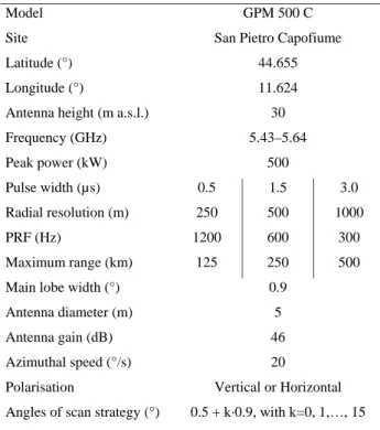
Table 1. Principal characteristics of San Pietro Capofiume radar.
Model GPM 500 C Site San Pietro Capofiume Latitude (°) 44.655 Longitude (°) 11.624 Antenna height (m a.s.l.) 30 Frequency (GHz) 5.43–5.64 Peak power (kW) 500 Pulse width (µs) 0.5 1.5 3.0 Radial resolution (m) 250 500 1000 PRF (Hz) 1200 600 300 Maximum range (km) 125 250 500 Main lobe width (°) 0.9
Antenna diameter (m) 5 Antenna gain (dB) 46 Azimuthal speed (°/s) 20
Polarisation Vertical or Horizontal Angles of scan strategy (°) 0.5 + k·0.9, with k=0, 1,…, 15
over reflectivity radar data to obtain rainfall rate estimations (see for example Fulton et al., 1998).
2.3 Beam shielding
Finally, the evaluation and correction for beam blocking is performed using a geometric optic approach based in the in-terception function proposed by Bech et al. (2003). In this study it has been applied the above-mentioned multi-layer model to retrieve the radar beam trajectory instead of as-suming a homogeneous vertical refractivity gradient for the whole air-layer. This refinement allows a more detailed de-scription of the radar beam behaviour introducing the possi-bility to simulate a wider variety of propagation effects such as beam-splitting.
In Fig. 1 is illustrated the complete correction procedure, emphasizing the input and output data and the additional re-quired information. The scheme will be called hereinafter ‘BDA’ (acronym of the three procedures included: Beam blocking, Dynamic map and Anaprop correction).
3 Datasets description
To evaluate the efficiency of the described methodology it has been applied to the rainfall rate measured by the C-band Doppler radar of San Pietro Capofiume, located in northern Italy (see Table 1 for details). The radar precipitation esti-mates have later been compared with raingauge data.
choice of the dynamic map vertical continuity test beam blockage correction
clear air echoes map beam blocking rates trajectory of the 3 dB beam lower limit
radiosounding data DTM historical reflectivity dataset corrected Z field polar volume of reflectivity decluttered through Doppler filter
Fig. 1. BDA scheme of reflectivity data correction. The two blue rectangles are the input data, the yellow rectangle contains the in-termediate products, the yellow circles are the three correction steps leading to the final output, the corrected reflectivity (Z) field.
The reflectivity data used in the analysis are provided ev-ery 15 min and collected using a short pulse of 0.5 microsec-onds and a pulse repetition frequency (PRF) of 1200 Hz. The radar pixels had a resolution of 250 m×0.9◦ and the mea-surements extended up to a maximum range of 125 km. As explained in the previous section, after the application of the correction the radar reflectivity is also contained in a bi-dimensional grid azimuth-range where each cell measures 250 m×0.9◦. The data are then resampled into a tempo-ral Cartesian grid of 250 m×250 m resolution, assigning the value of each polar cell to the nearest Cartesian cell. There-after this Cartesian grid is transformed to another one of lower resolution (1 km×1 km) more adequate to the original radar sampling, using the criterion of the maximum reflectiv-ity value into a box composed by 16 elementary cells.
The reflectivity Z is converted into rainfall rate R using a Z-R power-law relation Z=aRb, where the coefficients a and b are those indicated by Joss and Waldvogel (1970) for con-vective (a=500, b=1.5) and stratiform rain (a=250, b=1.5). Stratiform and convective events were distinguished subjec-tively by visual inspection on the radar data volumes. For sake of simplicity no attempt has been made to assign differ-ent Z-R relationships to differdiffer-ent pixels of the same image distinguishing between stratiform and convective precipita-tion type. This could be done with a classificaprecipita-tion technique such as those described by S´anchez-Diezma et al. (2001) or Rigo and Llasat (2004).
Finally, the hourly cumulated rainfall amount is obtained through weighted average of the five precipitation intensity values at 00, 15, 30, 45, 60 min before the nominal hour, where the extreme minutes of each hour (000and 600) weigh half of the others. This is done in order to take into account that half part of the 000and 600amounts do correspond to the
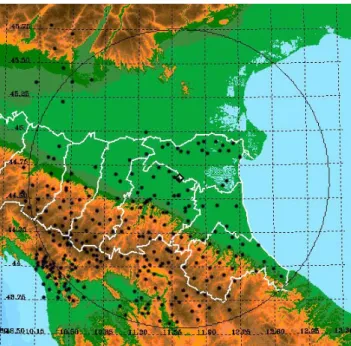
Fig. 2. Raingauges available for the analysis (black points) and radar coverage (black circle) in the North of Italy.
previous and next hour respectively unlike the other precip-itation amounts, which are recorded completely within the nominal hour.
Raingauge data were provided every 60, 30, or 15 min (see Tables 2 and 3). The amounts reported every 30 and 15 min were summed to obtain the corresponding hourly value. Most of the stations were located in the mountainous area and behind the mountains – in the SW part of the radar coverage –, so that beam blockage corrections could be eval-uated. The raingauges had tipping-bucket switches and were not warmed. Therefore some records might be mistaken dur-ing snow events. As explained later this has been taken into consideration in the analysis.
In Fig. 2 is represented the location of the raingauges and the radar maximum range circle.
4 Evaluation parameters
The comparison between raingauges and radar data has been performed through the visual inspection of rain maps and through a quantitative-statistical analysis based on the calcu-lation of some indices relative to the hourly-cumulated rain and to the event cumulated rain. The indices are: the bias, the root mean squared error, the fractional mean reduction and the fractional variance reduction.
Calling RGthe cumulated rain rate (over the hour or over the event) produced by the gauges and RR that estimated from reflectivity radar data in the corresponding cells, the indices used can be written as (Marzano et al., 2004):
Table 2. Raingauges available for the analysis divided by integra-tion time.
1st type 2nd type 3rd type
Integration time (min) 15 30 60
Number of raingauges 184 176 41
Total raingauges 401
Table 3. Raingauges taken into consideration for the analysis in each case study, detailing the number of observations in mountain blocked areas and in all areas (total).
Number of Apr Dec July Set July Set stations mount. mount. mount. mount. total total Available 401 401 401 401 401 401 Used 142 135 176 179 221 239
The bias <εR>
hεRi = hRR−RGi (1)
the root mean square error RMSE RMSE=
q
hε2Ri (2)
the fractional mean reduction FMR FMR=hRGi−hεRi
hRGi
(3) the fractional variance reduction FVR
FVR=σ 2R G−σ2εR σ2R G (4) where the angle brackets mean average over time and over the cells.
An efficient correction method should reduce the RMSE towards the “optimum limit” of 0, and it should produce val-ues of FMR and FVR tending to 1. In the analysis of the case studies, the RMSE calculated on the event-cumulated rain, is called RMSECUM. Because of the linear relation be-tween bias and FMR, in the next section, it has been con-sidered only the FMR that is normalized with respect to the mean gauges rainfall field. Moreover, when FMR is higher or lower than 1, the bias is respectively negative or positive.
The evaluation is limited to the raingauges located beyond 20 km from the radar site, to avoid the radar antenna sec-ondary lobes effect. Moreover, two different coverage ar-eas are taken into consideration: the whole 360◦angle and that limited between angles 135◦and 270◦, with respect to the north direction (in this case the minimum range is in-creased to 40 km). The second area represents the mountain-ous area, considered to highlight the behaviour of the algo-rithm in complex orography.
choice of the dynamic map vertical continuity test
clear air echoes map historical reflectivity dataset corrected Z field polar volume of reflectivity decluttered through Doppler filter
Fig. 3. Scheme of reflectivity data correction operative at ARPA-SIM (SA scheme).
5 Results and discussion
To evaluate the performance of the new BDA correction method it has been compared with another reference method that does not correct the radar data for beam blockage and does not consider either the approximate path of the beam to reduce the clutter.
This reference algorithm of clutter removal is actually op-erative at ARPA-SIM to correct data of San Pietro Capofi-ume and Gattatico radars. The algorithm is based on the use of a static clutter filter derived from a climatological map of non-precipitating echoes employed to select the antenna el-evation. Besides, the removal of residual anaprop clutter is done applying a vertical continuity test to the radar echo vol-umetric observations (see Fig. 3). This reference method will be called hereinafter “SA”.
The evaluation of the performance of the algorithms by us-ing raus-ingauges is uncertain at low temperatures when snow is present and tipping-bucket raingauges are not warmed. To address this problem, in the stratiform precipitation cases, comparisons were restricted to raingauges located at least 100 m below the minimum 0◦level during the event
consid-ered and having cumulated amounts higher than 1 mm. This restriction tries to avoid including snowfall observations mis-taken by the gauges though some sleet is likely to be included in the higher radar observations considered. However this ap-proach does not remove all the stations of interest, because raingauges sited in the valleys and beyond the mountains are conserved.
The first two events considered were stratiform cases: one occurred in spring, the other one in winter. In these cases, the analysis was limited to the mountainous and blocked ar-eas, because the propagation conditions were nearly standard and hence no significant changes between the BDA and SA outputs are produced in flat land areas.
The last two cases were convective summer events. In those cases superrefraction and ducting conditions were
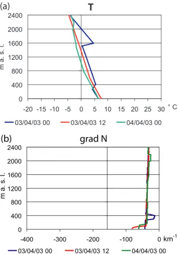
T
0 400 800 1200 1600 2000 2400 -20 -15 -10 -5 0 5 10 15 20 25 30 ° C m a . s . l . 03/04/03 00 03/04/03 12 04/04/03 00(a)
0 400 800 1200 1600 2000 2400 -400 -300 -200 -100 0km-1 m a . s . l . 03/04/03 00 03/04/03 12 04/04/03 00(b)
grad N
Fig. 4. Temperature (a) and refractivity vertical gradient profiles (b) obtained from radiosonde ascents during the 24-h period from 3rd 00:00 Z to 4th 00:00 Z April 2003.
clearly present due to the effect of a surface thermal inversion causing a strong surface duct. Therefore, these two cases are the most interesting to illustrate the effects of BDA method-ology.
5.1 Case study 1: April 2003
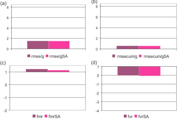
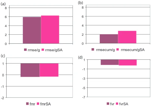
The first case presented took place from 2 to 4 April 2003. It was a clear stratiform event with minimum 0◦C level at around 1000 m (measured by radiosoundings) and normal re-fraction conditions, as it is visible in Fig. 4. The cumulated rainfall field, obtained using BDA method, seems to be more coherent and realistic as compared to SA output, because the shielding effect of mountains is reduced (Fig. 5). How-ever, no significant difference is shown by the raingauge-comparison RMSE and FVR indices, and the FMR is even slightly worse (Fig. 6).
One reason for this behaviour is probably the lack of cor-rection for vertical reflectivity variation. In fact, to avoid the mountain shielding effect in BDA method, the elevation is increased and the considered reflectivity values become less
Fig. 5. Cumulated rain of the April 2003 event, obtained using BDA (a) and SA (b) methods. In the SA precipitation field it is visible the shielding effect of the mountains; in BDA, after beam blockage correction, the field seems more coherent in the mountainous area and beyond. 0 2 4 6 8 rmse/g rmse/gSA
(a)
0 2 4 6 8 rmsecum/g rmsecum/gSA(b)
-2 -1 0 1 fmr fmrSA(c)
-4 -3 -2 -1 0 1 fvr fvrSA(d)
Fig. 6. Radar-raingauges comparison indices for the April event showing the performance of the BDA (dark pink) and SA (fuchsia) methods. Only raingauges located below 900 m a.m.s.l. (100 m below the minimum 0◦level) and in the mountainous sector (azimuth [135◦, 270◦], range >40 km) are considered. (a) RMSE normalised with respect to the mean gauge rainfall field for the hourly; (b) as a for the event cumulated rain rate; (c) FMR; (d) FVR indices.
representative of the ground value. So it seems plausible that during this event, at least in some cases, a blocked radar ob-servation nearer the ground might provide a more accurate
rainfall estimate than an unblocked observation aloft because of the presence of snowfall and sleet at higher altitudes.
T
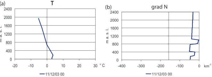
0 400 800 1200 1600 2000 2400 -20 -10 0 10 20 30 ° C m a . s. l. 11/12/03 00(a)
0 400 800 1200 1600 2000 2400 -400 -300 -200 -100 0 km-1 m a . s . l . 11/12/03 00(b)
grad N
Fig. 7. Temperature (a) and refractivity vertical gradient profile (b) obtained from radiosonde data during the 11th 00:00 Z December 2003.
Fig. 8. Cumulated rain of 10–11 December 2003 event, obtained using BDA (a) and SA (b) methods.
5.2 Case study 2: December 2003
The second event took place during 10 and 11 December 2003 and the minimum 0◦C level was approximately 600 m,
while the propagation conditions were normal (Fig. 7). Hence, the raingauges taken into consideration were those up to 500 m.
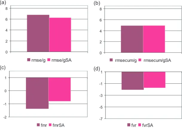
As in the previous case, the BDA output seems to be more coherent at the visual inspection (Fig. 8). In this case all the scores, calculated in the mountainous sector, were improved when the BDA methodology was applied: the RMSE and RMSECUM were reduced, patent improvement is visible in the FVR, the bias (positive, because FMR is lower than 1) decreased. The considerable reduction in FVR confirms the higher spatial coherence of BDA field beyond the orography obstacles.
Otherwise, the results, especially in this case, should be carefully considered. In fact, in the centre of the Fig. 8, that represents the event cumulated rainfall rate, a
remark-able concentric increase seems present, that evidences a clear bright band. Therefore, at longer ranges, the precipitation is probably snow and sleet. The bright band contribution is con-firmed by the positive bias and by the height of the midnight 0◦level (Fig. 9).
5.3 Case study 3: September 2003
The third case took place during 8 and 9 September 2003: the N gradient profiles, retrieved from the radiosoundings repre-sentative of the event, show deep superrefraction especially in the second day (moreover at midnight a temperature inver-sion is present), as pointed out in Fig. 10.
All scores yielded by the BDA method improved SA re-sults (except the FMR that does not provide relevant changes) either in the mountain region (Fig. 12) or in the 360◦domain (Fig. 13) presented separately for this case study. The im-provement, though still exists as pointed out by the scores, is less evident in the 360◦coverage: in fact, dealing with beam
0 2 4 6 8 rmse/g rmse/gSA
(a)
0 2 4 6 8 rmsecum/g rmsecum/gSA(b)
-2 -1 0 1fmr fmrSA
(c)
-7 -5 -3 -1 1fvr fvrSA
(d)
Fig. 9. Radar-raingauges comparison indices for the December event. Only the raingauges located below 500 m a.s.l. (100 m below the 0◦ level at midnight) and in the mountainous sector are considered. (a) RMSE normalised with respect to the mean gauge rainfall field for the hourly; (b) as a for the event cumulated rain rate; (c) FMR; (d) FVR indices.
T
0 400 800 1200 1600 2000 2400 -10 0 10 20 30 °C m a . s . l . 08/09/03 12 09/09/03 00 09/09/03 12(a)
0 400 800 1200 1600 2000 2400 -400 -300 -200 -100 0 km-1 m a . s . l . 08/09/03 12 09/09/03 00 09/09/03 12(b)
grad N
Fig. 10. Temperature (a) and refractivity vertical gradient profiles (b) obtained from radiosonde ascents during the 24-h period from 8th 12:00 Z to 9th 12:00 Z September 2003.
propagation and beam blocking, the BDA method produces the major effect in complex orography areas, and therefore, the scores improvement is smoothed by averaging over the whole radar domain (that includes a large flat land share). In either cases the higher impact is on RMSECUM, that is moreover, two-three times smaller than RMSE. This fact proves the higher usefulness of radar data in the estimate of
cumulated rainfall field, as compared to the instantaneous one.
Finally, the visual inspection of Fig. 11 reveals that the BDA precipitation field appears less affected from orography shielding (note the 170–270◦ and the 5–10◦ sectors of the image) than that obtained with the reference method SA.
Fig. 11. Cumulated rain of September 2003 event, obtained using BDA (left) and SA (right) methods. In the SA output, sectors 5◦–10◦and 170◦–270◦show the shielding effect of mountains, much less apparent in BDA field after the beam blockage correction was applied.
0 2 4 6 8 rmse/g rmse/gSA
(a)
0 2 4 6 8 rmsecum/g rmsecum/gSA(b)
-2 -1 0 1 fmr fmrSA(c)
-7 -5 -3 -1 1 fvr fvrSA(d)
Fig. 12. Radar-raingauges comparison indices for the September event, calculated in the mountainous sector. (a) RMSE normalised with respect to the mean gauge rainfall field for the hourly; (b) as a for the event cumulated rain rate; (c) FMR; (d) FVR indices.
5.4 Case study 4: July 2003
In 31 July 2003 the results were not so evident. The propaga-tion condipropaga-tions – showing an intense surface duct – are shown in Fig. 14 and the rainfall fields in Fig. 15. In particular, in the mountainous area the scores seemed to be worse (Fig. 16),
more specifically both the RMSE and FMR calculated from hourly values. A closer analysis revealed substantial tempo-ral variations throughout the event of the performance of the BDA algorithm.
Comparing the 17 p.m. hourly radar rainfall field ob-tained through BDA and SA methods with the rain gauges
0 2 4 6 8 rmse/g rmse/gSA
(a)
0 2 4 6 8 rmsecum/g rmsecum/gSA(b)
-2 -1 0 1fmr fmrSA
(c)
-7 -5 -3 -1 1 fvr fvrSA(d)
Fig. 13. Radar-raingauges comparison indices for the September event, calculated in the 360◦sector and beyond 20 km from radar site. (a) RMSE normalised with respect to the mean gauge rainfall field for the hourly; (b) as a for the event cumulated rain rate; (c) FMR; (d) FVR indices.
T
0 400 800 1200 1600 2000 2400 -10 0 10 20 30 °C m a . s . l . 31/07/03 00 31/07/03 12 01/08/03 00(a)
0 400 800 1200 1600 2000 2400 -600 -500 -400 -300 -200 -100 0 km-1 m a . s . l . 31/07/03 00 31/07/03 12 01/08/03 00(b)
grad N
Fig. 14. Temperature (a) and refractivity vertical gradient profiles (b) obtained from radiosonde ascents during the 24-h period from 31st 00:00 Z July to 1st 00:00 Z August 2003.
measurements, in the sector around the green line (–179◦ azimuth) shown by Fig. 17, it can be observed an overesti-mation, more evident in the new method. However, in that moment raingauges did not measure precipitation.
This was an unexpected result because at this time, due to anaprop risk, the BDA scheme chose nearly always the
second elevation scan, while in SA the first was mostly con-sidered (see the right panel of Fig. 18), and they were also expected lower reflectivity values.
The reason is probably another one: as it is visible at – 179◦ RHI (left panel of Fig. 18), overhanging precipitation is present and it is intercepted more widely from second
Fig. 15. Cumulated rain of July 2003 event, obtained using BDA (left) and SA (right) methods. 0 2 4 6 8 rmse/g rmse/gSA
(a)
0 2 4 6 8 rmsecum/g rmsecum/gSA(b)
-2 -1 0 1 fmr fmrSA(c)
-7 -5 -3 -1 1 fvr fvrSA(d)
Fig. 16. Radar-raingauges comparison indices for the July event, calculated in the mountainous sector. (a) RMSE normalised with respect to the mean gauge rainfall field for the hourly; (b) as a for the event cumulated rain rate; (c) FMR; (d) FVR indices.
elevation scan than from the first one. Therefore, a method to recognise such features could be very helpful in this case. Extending the analysis to the whole radar domain, and fo-calising it on the evening hours, Fig. 19, the indices become better in BDA with respect to SA output (except the FMR that is directly related to the bias). It seems clear that in the evening, when the anaprop contribution is stronger, the new methodology works well and the effects are visible too in flat
land areas. The improvement is partially due to the use of radiosounding information and to the modelling of the 3-dB beam lower limit path that conditions the elevation choice. This thesis is confirmed, in the same figure, by the yellow bars which represent the indices calculated on the output of a method that works analogous to BDA, except for assuming standard propagation to reproduce the beam path.
(a) 31/07/2003 17 BDA (b) 31/07/2003 17 SA
Fig. 17. Comparison between rainfall rates measured by the radar and by the raingauges at 31 July 2003 17:00 Z and using BDA (a) and SA (b) algorithms. The green line represents the RHI section illustrated in Fig. 18. In the area surrounding this line BDA produces precipitation where raingauges measure 0 mm. SA output is less affected from this problem.
azimuth:-170 Jul 31 16:04:43 2003
70 80 90 100 110 120
distance from radar (km) 0 2 4 6 8 10 he ig ht (k m ) -20 -15 -10 -5 0 5 10 15 20 25 30 35 40 45 50 55 60 dBZ (a) 120 60 0 60 120 km 120 60 0 60 120 km 12 0 6 0 0 60 12 0 k m 12 0 6 0 0 60 12 0 k m 0.5 1.4 2.3 3.2 4.1 deg
(b)
Fig. 18. Radar observations recorded on the 31 July 2003 16:04 Z (a): RHI at azimuth –170◦. (b): maps of antenna elevations chosen to retrieve rainfall rate from reflectivity data, for BDA and SA correction methods. The black line represents the RHI section. In the BDA map it is chosen the second elevation, nearly everywhere, which seems to intercept overhanging precipitation as is evidenced in the Fig. 17 from the comparison with the raingauges.
6 Conclusions
A post-processing operational method to correct single-polarisation radar reflectivity data for ground clutter and beam blocking has been evaluated in this paper. The method, called “BDA”, has among its main characteristics the detailed analysis of the beam shape and trajectory to build the correc-tion and the use of radiosounding informacorrec-tion as input data in the calculation of the radar beam path.
The advantages and limitations of the BDA method have been studied through the comparison with another previous method called “SA” based on static map clutter elimina-tion and anaprop removal, which neglects beam blocking er-rors and assumes standard refraction conditions for the radar beam. The two methods have been applied to four case stud-ies that took place at different seasons in the Po Valley (Italy). The analysis of the case studies was based on two tools:
vi-sual inspection and calculation of some statistic indices of comparison between the radar rainfall field and raingauge measures (FMR, FVR, RMSE).
In summary, through a comparison with raingauges the proposed BDA shows a tendency of the BDA method to re-duce the RMSE and the variance, and a growth of the bias (except for the December event). The choice of higher an-tenna elevation measurements of BDA with respect to SA and the lack of Vertical Profile of Reflectivity (VPR) cor-rection, is probably the reason of this bias increment. The improvement in the other indices, mainly in FVR, proves the higher coherency of the field obtained using BDA, con-firmed too from visual inspection of cumulated rainfall fields. It is also expected that, once removed the bias through ad-equate VPR correction the new method works consistently better than the older one. Moreover, taking into account re-alistic propagation conditions, this combined methodology is
0 2 4 6 8
rmse/g rmse/gSA rmse/gSP
(a)
0 2 4 6 8rmsecum/g rmsecum/gSA rmsecum/gSP
(b)
-2 -1 0 1 fmr fmrSA fmrSP(c)
-7 -5 -3 -1 1 fvr fvrSA fvrSP(d)
Fig. 19. Radar-raingauges comparison indices for the July event, calculated in the 360◦sector beyond 20 km from radar site and during the evening (from 17:00 Z to 23:00 Z) performance of the BDA (dark pink) and SA (fuchsia) methods. In yellow are the indices calculated on the output of a correction method analogous to BDA but considering standard propagation conditions during the event (SP). (a) RMSE normalised with respect to the mean gauge rainfall field for the hourly; (b) as a for the event cumulated rain rate; (c) FMR; (d) FVR indices.
efficient to avoid and remove anomalous propagation echoes. Finally, it should be taken into account the probability of overhanging rain, mainly during summer, as shown by one of the case studies. This could be done considering for ex-ample the Pohjola and Koistinen (2004) method to recognise such features through analysis of the VPR shape.
The version of the algorithm studied in the present work assumes as input the atmospheric data acquired in the 12 hours before and after the time of interest. This is a con-straint for real time applications. A possible solution is the use of NWP model forecasts of the refractivity field tendency (Bech et al., 2004), which could be complemented with the introduction of anaprop statistics in the simulation of the re-fractivity profile. Otherwise, it has been observed that the use of a detailed beam description produces the major effects in anaprop cases: a possible choice could be to use standard propagation or simply the average refractivity gradient, when anaprop has low probability, or when NWP model data are not reliable. After including these modifications, taking into account that the proposed methodology is not computation-ally expensive, this procedure is well suited for real-real time application.
Acknowledgements. This work was partially supported by CARPE
DIEM, a research project funded by the European Commission under the 5th FP (Contract N◦ EVG1-CT-2001-0045), and by the INTERREG IIIB programme through the RISK AWARE project (Contract N◦3B064) and was done within the framework of the EU-COST 717 action devoted to “Use of weather radar observations in NWP and hydrological models” and EU-COST -731 Action devoted to “Propagation of uncertainty in advanced meteo-hydrological forecast systems”.
Edited by: M. Bruen Reviewed by: two referees
References
Alberoni, P. P., Anderson, T., Mezzasalma, P., Michelson, D. B., and Nanni, S.: Use of the vertical reflectivity profile for identification of anomalous propagation, Meteorological Applications, 8, 257– 266, 2001.
Alberoni, P. P., Ducrocq, V., Gregoric, G., Haase, G., Holleman, I., Lindskog, M., Macpherson, B., Nuret, M., and Rossa, A.: Qual-ity and Assimilation of Radar Data for NWP – A Review, COST 717 document ISBN 92-894-4842-3, 38 pp, 2003.
Bean, B. R. and Dutton, E. J.: Radio Meteorology, Dover Publica-tions, 435 pp., 1968.
Bebbington, D.: DARTH EU Project Final Report, Part II. Anoma-lous Propagation Modelling, Essex University, UK, 18 pp., 1998. Bech, J., Codina, B., Lorente, J., and Bebbington, D.: The sensi-tivity of single polarization weather radar beam blockage correc-tion to variability in the vertical refractivity gradient, J. Atmos. Ocean. Tech., 20, 845–855, 2003.
Bech, J., Toda, J., Codina, B., Lorente, J., and Bebbington, D.: Using mesoscale NWP model data to identify radar anomalous propagation events, Proceedings of the 3rd European Radar Con-ference, Visby, Sweden, 310–314, 2004.
Bruen, M.: Using radar information in Hydrological Modelling, COST 717 WG-1 activities, Phys. Chem. Earth (B), 25, 1305– 1310, 2000.
Collier, C. G.: Applications of weather radar systems, John Wiley & Sons, 390 pp., 1996.
Collier, C. G.: Observations of sea clutter using an S-band weather radar, Meteorol. Appl., 5, 263–270, 1998.
da Silveira, R. B. and Holt, A. R.: A neural network application to discriminate between clutter and precipitation using polarisa-tion informapolarisa-tion as feature space, 28th Internat. Conf. on Radar Meteor., Amer. Meteor. Soc., Austin, Texas, 57–58, 1997. Fornasiero, A., Alberoni, P. P., Amorati, R., Ferraris, L., and
Tara-masso, A. C.: Effects of propagation conditions on radar beam-ground interaction: impact on data quality, Adv. Geosci., 2, 201– 208, 2005,
http://www.adv-geosci.net/2/201/2005/.
Fornasiero, A., Alberoni, P. P., and Bech, J.: Statistical analysis and modelling of weather radar beam propagation conditions in the Po valley (Italy), Nat. Hazards Earth Syst. Sci., 6, 303–314, 2006,
http://www.nat-hazards-earth-syst-sci.net/6/303/2006/.
Fulton, R. A., Breidenbach, J. P., Seo, D., Miller, D., and O’Bannon, T.: The WSR-88D Rainfall Algorithm, Wea. Forecasting, 13, 377–395, 1998.
Haddad, B., Adane, A., Sauvageot, H., Sadouki, L., and Naili, R.: Identification and filtering of rainfall and ground clutter echoes using textural features, Int. J. Remote Sensing, 25, 4641–4656, 2004.
Illingworth, A.: Improved precipitation rates and data quality by using polarimetric measurements, in: Weather Radar: Principles and Advanced Applications, edited by: Meischner, P., Springer-Verlag, chapter 5, 130–166, 2003.
Joss, J. and Waldvogel, A.: A method to improve the accuracy of radar-measured amounts of precipitation, Prepr., Radar Meteo-rol. Conf., 14th, 237–238, 1970.
Joss, J. and Waldvogel, A.: Precipitation measurement and hydrol-ogy, a review, in: Radar in Meteorolhydrol-ogy, edited by: Atlas, D., American Meteorol. Soc., Boston, chapter 29a, 577–606, 1990.
Joss, J. and Lee, R.: The application of radar-gauge comparisons to operational precipitation profile corrections, J. Appl. Meteor., 34, 2612–2630, 1995.
Marzano, F. S., Picciotti, E., and Vulpiani, G.: Rain field and re-flectivity vertical profile reconstruction from C-band radar volu-metric data, IEEE Trans. Geosci. Rem. Sens., 42(4), 1033–1046, 2004.
Michelson, D. B. and Sunhede, D.: Spurious weather radar echo identification and removal using multisource temperature infor-mation, Meteorol. Appl., 11, 1–14, 2004.
Pamment, J. A. and Conway, B. J.: Objective Identification of Echoes Due to Anomalous Propagation in Weather Radar Data, J. Atmos. Ocean. Tech., 15(1), 98–113, 1998.
Pankiewicz, G. S., Johnson, C. J., and Harrison, D. L.: Improving radar observations of precipitation with a Meteosat neural net-work classifier, Meteorol. Atmos. Phys., 76, 9–22, 2001. Pohjola, H. and Koistinen, J.: Identification and elimination of
over-hanging precipitation, Proceedings of the 3rd European Radar Conference, Visby, Sweden, 91–93, 2004.
Rigo, T. and Llasat, M. C.: A methodology for the classification of convective structures using meteorological radar, Nat. Hazards Earth Syst. Sci., 4, 59–68, 2004,
http://www.nat-hazards-earth-syst-sci.net/4/59/2004/.
Rossa, A. M.: COST-717: Use of radar observations in hydrological and NWP models, Phys. Chem. Earth (B), 10–12, 1221–1224, 2000.
Ryhzkov, A. V., Schuur, T. J., Burgess, D. W., Heinselman, P. L., Giangrande, S. E., and Zrnic, D. S.: The joint polarization exper-iment: polarimetric rainfall measurement and hydrometeor clas-sification, Bulletin American Meteorol. Soc., 86, 809–824, 2005. Ryhzkov, A. V. and Zrnic, D. S.: Polarimetric rainfall estimation in the presence of anomalous propagation, J. Atmos. Ocean. Tech., 15, 1320–1330, 1998.
S´anchez-Diezma, R., Sempere-Torres, D., Delrieu, G., and Za-wadzki, I.: An improved methodology for ground clutter sub-stitution based on a pre-classification of precipitation types, 30th Internat. Conf. on Radar Meteor., M¨unich, Germany, Amer. Me-teor. Soc., 271–273, 2001.
Smith Jr., P. L.: On the minimum useful elevation angle for weather surveillance radar scans, J. Atmos. Ocean. Tech., 15, 841–843. 1998.
Steiner, M. and Smith, J. A.: Use of three-dimensional reflec-tivity structure for automated detection and removal of non-precipitating echoes in radar data, J. Atmos. Ocean. Tech., 19, 673–686, 2002.
Todini, E.: A Bayesian technique for conditioning radar precipita-tion estimates to rain-gauge measurements, Hydrol. Earth Syst. Sci., 5, 187–199, 2001,
http://www.hydrol-earth-syst-sci.net/5/187/2001/.
Wesson, M. and Pegram, G. S.: Radar rainfall image repair tech-niques, Hydrol. Earth Syst. Sci., 8, 220–234, 2004,