Development of an aerodynamic/RCS framework for the preliminary design of a hypersonic aircraft

Development of an Aerodynamic/RCS Framework for the

Preliminary Design of a Hypersonic Aircraft

by

Daniel L. DiCara

Submitted to the Department of Aerospace Engineering in partial fulfillment of the requirements for the degree of

Master of Science in Aerospace Engineering at the

MASSACHUSETTS INSTITUTE OF TECHNOLOGY

@

Massachusetts

May 2006

Institute of Technology 2006. All rights reserved.

A uthor ... ... ... Department of Aerospace Engineering

May 26, 2006 A Certified by ... Jaime Peraire Professor Thesis Supervisor . i Accepted by... MASSACHUSETTS INSTITUTE OF TECHNOLOGY

OCT 15

2008

LIBRARIES

Chairman, Jaime Peraire Department Committee on Graduate Students

ARCHIVES

Development of an Aerodynamic/RCS Framework for the

Preliminary Design of a Hypersonic Aircraft

by

Daniel L. DiCara

Submitted to the Department of Aerospace Engineering on May 26, 2006, in partial fulfillment of the

requirements for the degree of

Master of Science in Aerospace Engineering

Abstract

The design of hypersonic airbreathing aircraft pushes the envelope of current state-of-the-art aerospace propulsion and materials technology. Therefore, these aircraft are highly integrated to produce adequate thrust, reduce drag, and limit surface heating. Consequently, every aircraft component (e.g., wings, fuselage, propulsion system) is sensitive to changes in every other component. Including Radar Cross Section (RCS) considerations further complicates matters. During preliminary design, this requires the rapid analysis of different aircraft configurations to investigate component inter-actions and determine performance trends. This thesis presents a framework and accompanying software for performing such an analysis. The intent is to optimize a hypersonic airbreathing aircraft design in terms of aerodynamic performance and RCS. Computational Fluid Dynamics (CFD) and Computational Electromagnetics (CEM) are the two main framework software components. CFD simulates airflow around the aircraft to analyze its aerodynamic performance. Alternately, CEM simulates the elec-tromagnetic signature of the aircraft to predict its RCS. The framework begins with the generation of a three-dimensional computer aided design aircraft model. Next, a grid generator discretizes this model. The flow simulation is performed on this grid and the aircraft's aerodynamic characteristics are determined. Flow visualization aids this determination. Then, aircraft geometry refinements are made to improve aero-dynamic performance. Afterward, CEM is performed on aeroaero-dynamically favorable designs at various aspect angles and frequencies. RCS values are determined and used to rank the different configurations. Also, inverse synthetic aperture radar images are generated to locate major scattering centers and aid the design refinement. The de-sign loop continues in this fashion until an acceptable aircraft dede-sign is achieved. The NASA X-43A test vehicle was used to validate this preliminary design framework.

Thesis Supervisor: Jaime Peraire Title: Professor

Acknowledgments

I would like to thank MIT Lincoln Laboratory and the Lincoln Scholars Committee for funding my graduate work and providing valuable feedback over the course of my research. Two other people at Lincoln Laboratory I would like to thank are Dr. Jack Fleischman and Dr. Hsiu Han. Jack was my group leader at Lincoln Laboratory when I applied to the Lincoln Scholars Program. I cannot thank him enough for supporting my entrance into the graduate program at MIT and providing me with a challenging and exciting research topic. Furthermore, Hsiu was my Lincoln Laboratory advisor during the course of my graduate work. He was an excellent resource and provided much needed instruction on all topics having to do with Electromagnetics. Having an aerospace engineering background, I was fairly inexperienced in this area prior to entering graduate school. I am very grateful for his patience and effort in instructing me in this field.

I am also thankful for the software installation and support given by William Jones and Karen Bibb at the NASA Langley Research Center. Bill provided me with the GridEx software that was a crucial component of my design framework. Despite his very busy schedule, he was quick to fix any problems that came up and provide guidance whenever necesary. Karen also took a lot of time out of her busy schedule to provide me with the FELISA Hypersonics code, also a crucial component of my design framework. Karen did an excellent job of modifying the code so it would compile and run on the Aerospace Computational Design Lab (ACDL) cluster. Without this help, simulation times would have easily taken an order of magnitude longer than using the

10 node ACDL cluster.

Last, but definitely not least, I would like to thank several members of the ACDL. For instance, Bob Haimes and Garret Barter were invaluable in assisting me with all of my computer related issues. Bob provided me with much needed installation and user support for VisualS. This tool is responsible for all of the flow visualizations presented in this thesis. Bob also provided advice and support on everything from

ProEngineer to system backups. I really appreciate his willingness to help me with problems that inevitably arise when trying to integrate a multitude of software into a coherent framework. Similarly, Garrett provided extensive time and effort into configuring my laptop, desktop, and the cluster to accomodate my needs. Also, I had two hard drive failures during my graduate studies, and Garrett was very helpful in getting me back online. He also put up with all of my day to day questions about how to print, using latex, and just about anything else you could think of. Lastly, I am very grateful for my advisor, Professor Jaime Peraire. His encouraging advice and enthusiasm about my research kept me motivated even when things were not going well. I also appreciated his knowledgable guidance and his ability to convey difficult subject matter to me in terms I could understand. Finally, Professor Peraire's friendly nature made him a real pleasure to work with.

Contents

1 Introduction 13

1.1 Hypersonic Aerodynamics ... 14

1.2 Scramjet Propulsion ... 17

1.2.1 Engine Description ... .. 18

1.2.2 Combustor Inlet Model ... 20

1.2.3 Combustor Exit Model ... 22

1.3 Radar Cross Section Reduction ... 25

1.3.1 Radar Equation ... 26

1.3.2 Radar Cross Section ... 27

1.3.3 Scattering Mechanisms ... .... 29

1.3.4 RCS Reduction Techniques .... . . ... .. . . 30

2 Preliminary Design Framework 33 2.1 3D Computer Aided Design Solid Modeling . ... 33

2.2 Grid Generation ... . . . .... . . ... . . . . . . 35

2.3 Flow Simulation ... . .. . . . .... .. ... .. . . . . 36

2.4 RCS Signature Prediction ... 36

3 X-43A Trade Study 39 3.1 Compression System ... 40

3.1.1 Aerodynamic Performance . . . ... . . . 42

3.2 Expansion System ... 51

3.2.1 Aerodynamic Performance ... .. 52

3.2.2 RCS Performance ... 53

List of Figures

1-1 1-2

X-43A Hypersonic Airbreathing Aircraft [8] Scramjet Engine Stages [3] . . . .

2-1 Aerodynamic/RCS Framework Outline . . . 2-2 EM Signature Prediction Techniques . . . .

X-43A Flight Test Aircraft Photograph [12] External Compression System Design . . . . Internal Compression System Design . . . . Total Pressure Ratio Design Comparison . . Kinetic Energy Efficiency Design Comparison

. . . . . 4 0 . . . . . 4 0 . . . . . 4 1 . . . . . 4 2 . . . . . 4 3 Mach Number Visualization for IFA = 600 LEA = 90 w/Ramp . . .

Mach Number Visualization for IFA = 1350 LEA = 90 w/out Ramp Density Visualization for IFA = 600 LEA = 90 w/Ramp . . . . Density Visualization for IFA = 1350 LEA = 90 w/out Ramp . . . Pressure Visualization for IFA = 600 LEA = 9' w/Ramp . . . . Pressure Visualization for IFA = 1350 LEA = 90 w/out Ramp . . . Median RCS Design Comparison . . . . Total Pressure Ratio Design Comparison Refinement . . . . Kinetic Energy Efficiency Design Comparison Refinement . . . . Leading Edge Angle RCS Comparison . . . .. Internal Ramp Configuration RCS Comparison . . . . Lift-to-Drag Ratio ... 3-1 3-2 3-3 3-4 3-5 3-6 3-7 3-8 3-9 3-10 3-11 3-12 3-13 3-14 3-15 3-16 3-17

3-18 Scramjet Engine Thrust ... . . ... . 53 3-19 Tail-End HC Configuration ... ... 53 3-20 Pressure Visualization for IFA = 1200 LEA = 9' No Ramp w/out HC . 55 3-21 Pressure Visualization for IFA = 120' LEA = 90 No Ramp w/HC . . . 55 3-22 Tail End Configuration RCS Comparison . ... 56 3-23 2D and 3D Flow Visualizations ... ... 57 3-24 Control Surface Configuration RCS Comparison . ... 58

List of Tables

Chapter 1

Introduction

Preliminary aircraft design requires efficient methods for estimating aircraft perfor-mance. Important performance considerations are lift, drag, stability, control surface authority, and propulsion system selection and integration. In military aircraft design, Radar Cross Section (RCS) is also crucial. These design considerations are highly cou-pled - improving one may adversely affect the others. Therefore, refining an aircraft design requires extensive simulation to examine trade-offs between different aircraft configurations. Unfortunately, predicting aerodynamic performance using Computa-tional Fluid Dynamics (CFD) is typically time-consuming. Similarly, predicting air-craft RCS using Computational Electromagnetics (CEM) takes a considerable amount of time. As a result, low fidelity tools are generally used in preliminary aircraft de-sign, and such tools may inaccurately predict aircraft performance, adversely affecting crucial design decisions. Therefore, this thesis provides a framework and accompany-ing suite of software to rapidly perform CFD and CEM simulations for preliminary aircraft design in terms of aerodynamic and RCS considerations.

To demonstrate the utility of this framework and the accompanying software, a case study was performed using a baseline aircraft configuration as a starting point. An idea underlying this thesis is to look towards the future of military aircraft design. Most would agree that future military air vehicles will need to fly higher, farther, and faster. The epitome of this concept is the NASA X-43A. This experimental aircraft

flies at hypersonic speeds (> Mach 5) within the atmosphere. It employs a scram-jet propulsion system, which is considered the most likely candidate for hypersonic airbreathing flight in production aircraft in the future. Additionally, the X-43A com-pleted two successful flight tests during my graduate studies lending credence to the viability of scramjet engine technology. Furthermore, photographs and diagrams of the X-43A are available in the open literature and were used in producing this thesis. Therefore, a canonical hypersonic airbreathing aircraft configuration was constructed based on the X-43A design; wherein the configuration was refined using the prelimi-nary design framework presented herein.

1.1

Hypersonic Aerodynamics

In Reference [5], Anderson identifies five flow phenomena that become significant as the freestream Mach number is increased through hypersonic values. They are the fol-lowing: thin shock layers, entropy layers, viscous interactions, high-temperature flows, and low-density flows. The influence of these phenomena distinguish hypersonic flow from other flow regimes. Firstly, thin shock layers result from the high Mach numbers encountered in hypersonic flow. According to oblique shock wave theory, higher flow Mach numbers produce smaller shock-wave angles. Consequently, sharp aircraft edges in a hypersonic flow produce oblique shock waves that reside very near the aircraft's surface. In certain instances, these shallow oblique shocks may interact with the vis-cous boundary layer. Alternately, blunt aircraft edges and nose cones in hypersonic flows produce what is called an entropy layer. These blunt surfaces effectuate strong curved bow shocks. Entropy increases across a shock and the magnitude of this in-crease depends on the shock strength and hence the shock-wave angle. Therefore, the curvature of the bow shock generates an entropy gradient (layer) normal to the aircraft surface that also interacts with the boundary layer.

Shallow oblique shock waves and entropy layers are not the only aspects of hy-personic flow that have the potential to affect the boundary layer. For instance, the

internal energy of hypersonic freestream fluid particles is small in comparison to their kinetic energy [1]. This kinetic energy is dissipated in the boundary layer and mani-fests primarily as a temperature increase. This increase in temperature has two effects: (i) it increases the viscosity of the fluid, and (ii) it decreases the density. Both effects feed off of one another to increase the boundary layer thickness. In extreme cases, the boundary layer may even merge with the shock wave. This interaction between the boundary layer and the outer inviscid flow region is termed viscous interaction. High-temperature flows are also a result of the increased temperature in the boundary layer. If the temperature is high enough, the internal vibrational energy modes of the fluid particles may become excited. Furthermore, dissociation of the fluid molecules and even ionization may take place. These are often referred to as real gas effects and they act to reduce the thickness of the boundary layer. Finally, most hypersonic aircraft travel to the edge of the atmosphere or even into outer space. At these high altitudes, density of the air is low enough to invalidate the assumption that air is a continuum (continuous medium). In these instances, the field of rarefied gas dynamics must be used to simulate the flow accurately.

The flow does not have to exhibit all of these phenomena at once to be con-sidered hypersonic. However, as the Mach number approaches higher values, all of these phenomena emerge and become significant. Thus, CFD codes of increasing fi-delity/complexity are required. For the hypersonic airbreathing aircraft studied in this thesis, relatively low hypersonic Mach numbers (< Mach 10) are analyzed. The reason for this is twofold: (i) the atmosphere must be dense enough to provide adequate oxy-gen to the airbreathing propulsion system, and (ii) the surface temperatures on the aircraft must be manageable for the given state-of-the-art materials employed. For a typical flight, this requires an altitude of 100 kft where air is still considered a contin-uum. At this altitude, relatively low Mach numbers are necessary to achieve sustained hypersonic flight without the aircraft overheating. Consequently, strong viscous inter-actions, low-density, and high-temperature flow effects have a limited significance in the case of hypersonic airbreathing aircraft. As scramjet engine technology matures

and materials designed to operate at higher temperatures are developed in the future, perhaps higher Mach numbers for these type of vehicles can be achieved. However, given current materials and scramjet engine limitations for hypersonic aircraft, the chosen freestream Mach number simulated in this thesis is reasonable. Therefore, the inviscid hypersonic flow solver (FELISA) utilized in this thesis provides adequate results for preliminary hypersonic airbreathing aircraft design.

The disparity between conventional and hypersonic airbreathing aircraft configu-rations reflects the aerodynamic differences just described. For instance, conventional aircraft can be broken down into distinct components (e.g., wings, fuselage, horizontal and vertical tail, engines). In conventional aircraft design, these components can be designed and analyzed separately with modest consideration of the interactions be-tween the different aircraft parts. This is not true when designing hypersonic aircraft. The components of hypersonic aircraft must be highly coupled in order to manage the harsh hypersonic flow environment [11]. For instance, in scramjet engine design, the airbreathing engine is typically integrated into the airframe to reduce wave drag and take advantage of the bottom compression/expansion surfaces of the aircraft. Also to reduce wave drag, blended wing body configurations and highly swept control surfaces are typically employed. A design that implements these ideas is the X-43A given in Figure 1-1.

First of all, notice that distinct wings are unnecessary for providing lift. High pressure air behind the leading edge shock exerts enough force (lift) on the underside of the aircraft to support its weight [5]. Furthermore, the engine is integrated into the airframe. The under-surface of the aircraft forward of the engine has been designed to efficiently compress the air through a series of oblique shocks. Similarly, aft of the engine, the under-surface has been designed to efficiently expand the combustion gases to produce additional thrust. Finally, the control surfaces are significantly swept back to reduce wave drag. These are common traits of hypersonic airbreathing aircraft that

X-43A B

NASA Dryden Flight Research Center Graphics Collection http://www.dfrc. nasa.gov/gallery/graphics/index.html

created April 6, 2004 by Tony Landis

X-43A 3-view

Figure 1-1: X-43A Hypersonic Airbreathing Aircraft [8]

1.2

Scramjet Propulsion

The typical modern jet engine requires a compressor that consists of alternating rows of rotating (rotor) blades and stationary (stator) vanes. The compressor provides a rise in static pressure to the combustor inlet. This static pressure rise is necessary for efficient combustion. A turbine residing behind the combustor also contains alternating rows of rotor blades and stator vanes. It extracts a portion of the energy from the hot combustion gases to power the compressor, wherein the remaining energy is discharged as useful work in the form of thrust. An advantage of hypersonic aircraft design is that this compressor and turbine hardware is unnecessary. A hypersonic aircraft is designed to take advantage of normal and/or oblique shock waves in the flow that provide adequate compression prior to the combustor inlet. This is known as the

"ram effect," and consequently, engines of this type are called ramjets. Scramjets (Supersonic Combustion RAMJETs) are a type of ramjet in which air entering the

combustor is supersonic. For vehicles traveling at hypersonic speeds (4 Mach 6), it is inefficient to slow the air to subsonic speeds prior to combustion. Therefore, scramjet engines are typically the chosen propulsion system for hypersonic airbreathing aircraft.

1.2.1

Engine Description

Compression Combustion

1 3 4

Expansion

9

Figure 1-2: Scramjet Engine Stages [3]

A generic scramjet engine is illustrated in Figure 1-2. Similar to a conventional jet engine, a scramjet performs three main functions: compression, combustion, and ex-pansion. The unconventional aspect of scramjets is their incorporation of the vehicle's airframe into the compression and expansion processes. Properly shaping the under-side of the aircraft prior to the engine inlet and aft of the engine outlet significantly reduces engine size and drag. In the figure, numbers are prescribed to each engine stage and will be used to denote the location of various fluid state variables mentioned in the discussion that follows. Furthermore, Table 1.2.1 provides a description of each engine stage.

FELISA simulates the flow field up to the combustor entrance (station 3). Since the flow is supersonic throughout the combustor, boundary conditions prescribed at

Stage Description 0 Freestream Conditions

External Compression Begins 1 External Compression Ends

Diffuser Entry 3 Diffuser Exit Combustor Entry 4 Combustor Exit Nozzle Entry 9 Nozzle Exit

External Expansion Begins 10 External Expansion Ends

Table 1.1: Scramjet Engine Reference Station Descriptions [3]

the combustor entrance will not affect the flow. However, a thermodynamic model of the compression system was derived to determine the desired fluid state (density, ve-locity, energy, pressure, and speed of sound) at the combustor entrance, as more fully described herein. The results from the compression system model will be compared to the CFD simulated fluid state. Then, the compression system will be iteratively modified to achieve the desired fluid state at the combustor inlet. Otherwise, combus-tion will be inefficient and adequate thrust will not be produced. A descripcombus-tion of the compression system model will be described below.

The actual combustion process will be treated as a black box in the CFD simula-tion, wherein a model of the combustor has been calibrated to arrive at the desired combustor exit fluid state. Unlike the combustor entrance, boundary conditions at the combustor exit will influence the fluid state in the CFD simulation. Typical scramjet engine operating conditions were gleaned, in most part, from Reference [3]. This design methodology will also be described below. Finally, ambient air properties were needed to evaluate the engine modeling equations. A typical flight altitude for hy-personic aircraft is 100 kft. Therefore, properties of the "U.S. Standard Atmosphere 1976" at 100 kft were used. These properties include To = 227 K, Po = 1090 Pa,

1.2.2

Combustor Inlet Model

Typically, a limiting factor in the design of a compression system is the cycle static temperature ratio (4 = 1). This is the ratio of static temperature at the combustor inlet to the ambient air temperature. For scramjet engines, acceptable combustor inlet temperatures typically range from 1440 K to 1670 K [3]. Consequently, the cycle static temperature ratio is 6.3 < b < 7.4. The ratio used in this model is

'

= 7. Furthermore, two assumptions that sacrifice very little accuracy are that compression is adiabatic and the fluid is a calorically perfect gas. The adiabatic compression assumption permits the conservation of total enthalpy during the compression process. Furthermore, a calorically perfect gas has a constant ratio of specific heats. The ratio used in this analysis will be > = 1.36. These assumptions help simplify the following derivation.

Definitions of the first two fluid state variables at the combustor inlet are given here. Speed of sound and specific internal energy are given in Equations 1.1 and 1.2, respectively. The speed of sound requires the specific gas constant for air, R = 287 J

kgK '

and the specific internal energy is defined using the specific heat of air at constant

volume, C,, R -797 J

c-1 kg.K

a3 = VyRT3=

/R

7To (1.1)

e3 = CT 3 (1.2)

Deriving the velocity at the combustor can be accomplished by using the conser-vation of energy given in Equation 1.3.

pouoAo (ho + ) + rhb+ (hb ) + + p 3U3A3 (h 3 + V (1.3)

Assuming no mass addition eliminates the summation term (Z nb = 0) and results

in the following simplification: rh = pouoAo = p3u3A3. Furthermore, the adiabatic

external work is being applied to the fluid, the work term is eliminated (W = 0). Fi-nally, the calorically perfect gas assumption permits the replacement of enthalpy with temperature and specific heat (ho = C,,To and h3 = CcT3). Applying these

assump-tions and rearranging Equation 1.3 gives Equation 1.4 for velocity at the entrance to the combustor.

V3 = V2 - 2CpTo ( - 1) (1.4)

Fluid velocity will be assumed parallel to the engine walls in the axial direction. Therefore, only the x-component of velocity will be assumed nonzero resulting in the three components of velocity given by Equations 1.5-1.7.

us = V3 (1.5)

v3 = 0 (1.6)

w3 = 0 (1.7)

Next, the static pressure ratio is defined using a compression system efficiency term,

c = hh. This term relates the ideal (i.e. isentropic) change in static enthalpy to the

h3-ho"

real (non-isentropic) change in enthalpy that occurs during the compression process. This efficiency term can be reformulated to yield Equation 1.8 in terms of an ideal temperature ratio.

Cpc (T3 - TX) T

c - To - = 0 (1 - o) + 7c (1.8)

C, (T3 - To) - 1 To

Subsequently, Gibbs equation (Equation 1.9) evaluated for an isentropic process yields the compression system static pressure ratio given in Equation 1.10.

dP dT dP Tds = dh - = ds = Cpc- R (1.9) p T P T3 P3 P3 T3 R (1.10) s - s = 0 = Cpcln- -R In =o = T, Po P0

I

p1'7)'c (1.10)

As a result of the ideal gas assumption, density is then computed as given in Equation 1.11. All the necessary state variables for the combustor entrance have now been defined in Equations 1.1-1.2, 1.5-1.7, and 1.10-1.11.

P3

P3 =(1.11) RT3

Two compression system figures of merit will be used to gauge the performance of different inlet configurations. These are total pressure ratio and kinetic energy efficiency. The total pressure ratio is simply the ratio of total pressure at the combustor entrance to the total pressure in the freestream. This is given in Equation 1.12. The kinetic energy efficiency is simply the ratio of velocity that would be achieved in isentropic compression to the actual velocity that is achieved at the combustor entrance. This is given in Equation 1.13. Ultimately, an efficient compression system converts the kinetic energy in the freestream into a large pressure and density rise at the combustor entrance, with as small a rise in temperature as is possible.

PT3 _

+

--

1

1 -1C- + 2 (1.12) 1 + N2 1 M2 PTO 2 0 V=2 V2 - 2Cpc (T - To) (113) V20 V0

1.2.3

Combustor Exit Model

A few decisions were made before modeling the combustion process. For instance, hydrogen fuel (H2) was modeled in this analysis due to its high heat of reaction (hpR =

119,954 kJ/kg Fuel). Additionally, hydrogen is a typical scramjet engine fuel and was used to power the X-43A. Next, an appropriate fuel-to-air ratio (fat) was derived using stoichiometric (ideal) combustion in which all the available fuel and requisite oxygen are consumed. Equation 1.14 provides this ratio for hydrocarbon fuels [3]. The fuel-to-air ratio for hydrogen fuel was determined by plugging in x = 0 and y = 2 for the

number of carbon and hydrogen atoms, respectively, in molecular hydrogen.

fst = 36x+3y = 0.0291 (1.14)

103 (4x + y)

Finally, as had been assumed in the compression process, air during combustion is assumed to be a calorically perfect gas. Therefore, a typical value of the ratio of specific heats for scramjet engines is Yb = 1.238. Consequently, the specific heats at constant pressure and volume were now known: Cpb = = -bR 1493 J and Cb

R1= 1206 J.

7b-1 kg-K

Combustion was modeled as a constant pressure deflagration. Therefore, pressure at the combustor exit is immediately known.

P4 = P3 (1.15)

Next, the combustor exit velocity is derived using conservation of momentum as given in Equation 1.16.

P3A3 + (p3u3A3) u3 + r nhbUb + F = P4A4 + (p4u4A4) u4 (1.16)

Devices in the combustor, such as fuel injectors and mixers, protrude into the flow path and cause drag. This is accounted for through a burner effective drag coefficient of the form C A- where A, is the wetted area of the internal combustor surfaces. Therefore, the force in this equation is given by F = -P3u'A3Cf. A- Second, the2 3 A₃ o

only mass addition is fuel. Therefore, E rhbUb is replaced with tif uf. In addition, the

fuel-to-air ratio can be defined in relation to the combustor inlet, exit, and fuel mass flow rates. This is given in Equation 1.17.

rif m4 - 3

- = .7i4 = mi (1 + f) (1.17)

Uf = _{Vf), Equation 1.16 can be reformulated using these considerations and the fact}

that

ni3

= P3u3A3 and

ni4

= p4u4A4. The result of these simplifications is given in

Equation 1.18.

P(A3 -A4) _{+4 = 1-+f. Y' CI + f A A3 (1.18)}

4 = V3 A V (1 +- f ) + 1 f 2 (1 +

f

1)

The first term within the brackets can often be neglected. Furthermore, a reasonable assumption for the fuel entrance velocity in comparison to V3 is - _V3 = 0.5. Lastly, a

conservative estimate of the burner effective drag coefficient is Cf - -= 0.1. Velocity at the combustor exit can now be defined using these assumptions. Equations 1.19

-1.21 give the three components of velocity.

4 = V4 = V3

_{V4 =}

₁₌

_f

V C

_{(1+ f)}

A = 0.937V₃ (1.19)

v4 = 0 (1.20)

W4= 0 (1.21)

Temperature at the combustor exit is defined using conservation of energy as given in Equation 1.3. Unlike the compression system, combustion is not adiabatic and includes mass addition through the incorporation of fuel. Therefore, heat addition is given by

Q

= rbrnfhPR where irb is the burner efficiency. A conservative estimate of the burner efficiency is 80%. Since mass addition occurs, a reference temperature

(TO = To = _{227 K) is used to accurately estimate the absolute static enthalpy. Finally,}

the work term can be neglected resulting in Equation 1.22.

nA3 [Cpb (T3 - T) + + m f [hif + + -brnfhhpR = r 4 [Cpb (T4 - TO) +

(1.22) The absolute sensible enthalpy of the fuel entering the combustor is hf. It is often neglected in comparison to Q which contains a much higher fuel heat of reaction term,

the temperature at the combustor exit in Equation 1.23.

T3 1 V[2 V 2

T4 +f fhPR +f bT+(+fV2) K] 2pb

(1.23)

1 + f CpbT3 V2

2

2pb

After computing T4, the speed of sound, density and internal energy of the fluid at

the combustor exit can be readily defined as given in Equations 1.24-1.26. Therefore, given the achieved fluid state at the combustor entrance from the CFD simulation, an appropriate fluid state at the combustor exit can be computed using Equations 1.15, 1.19-1.21, and 1.24-1.26. These values can then be enforced in the CFD simulation to accurately predict the scramjet engine's performance. The figures of merit used for gauging such performance will be Lift-to-Drag ratio (L/D) and thrust.

a4 = V/bRT4 (1.24)

P4

P4 = (1.25)

RT4

e4 CvbT4 (1.26)

1.3

Radar Cross Section Reduction

Before tackling RCS reduction techniques, a brief discussion concerning radar system performance, RCS, and the appropriate physics involved is warranted. To begin, radar stands for radio detection and ranging. As the name implies, a radar emits radio waves to detect, locate, and track targets. A target in the radar beam intercepts these EM waves and a current along the target's surface is induced. Behaving like an antenna, the target's surface current radiates its own electric field known as the scattered field [4]. RCS (often denoted by u) is a measure of this scattered field intensity compared to that of the radar emitted electric field incident on the target. The scattered field then makes its way back to the radar. The radar receiver intercepts and processes this field and depending on the Signal to Noise Ratio (S/N or SNR), a detection may occur.

Location, velocity, and other information about the target may also be obtained from these detections. A mathematical description of this process is given by the radar equation that follows.

1.3.1

Radar Equation

Some terms used in defining the radar equation are provided below.

* T, = Transmitter and R, - Receiver * PT - Transmitted Power

" PID _ Transmitted Power Density Incident on the Target

* Ps - Scattered Power at the Target

* pR E Scattered Power Density at the Radar * PR: - Scattered Power Incident on the Radar

The scattered power, given in Equation 1.27, is a measure of the scattered electric field strength. In this equation, RT. is the range to the target, GT, is the gain of the transmitting antenna, and a is the RCS of the target. The 4rR42 term in the denominator is known as the spreading loss. The transmitted power is distributed on the surface of a sphere centered at the radar with a radius RTX. Therefore, power density on the sphere decreases as distance from the radar increases. Counteracting this effect, the gain term represents the focusing capability of the transmitting antenna in comparison to an isotropic antenna.

Ps = PTGT (1.27)

Extending this equation to represent the scattered power density at the radar involves the addition of another spreading loss term. This accounts for the return trip from the target back to the radar. The result is given in Equation 1.28.

D PTxGTx

pD=4P _{S 47 R~q} 4 R (1.28)

The receiving antenna also has an associated gain, GR, that is incorporated into a term coined the effective antenna aperture. This is given in Equation 1.29. The scattered power received by the radar is then given by Equation 1.30.

Ae = - (1.29)

4r

PT.GTxr JAe PTxGTxGIR.A 2

Pax = r47rR = (4)3xR (1.30)

4wRL 4wR2

(4)

3 4R 2R

Monostatic radars share the same transmit and receive antenna. Therefore, the fol-lowing simplifications apply: RT~ = RRx = R and GTx~ = G = G. This reduces Equation 1.30 to Equation 1.31 that is commonly referred to as the radar equation.

PTXG2aA2

PRx = (1.31)

(47r)3R4

1.3.2

Radar Cross Section

A typical expression for RCS is given in Equation 1.32 [6]. In this equation, Es is the scattered electric field and Ei is the radar transmitted electric field incident on the

target.

r= 4R2 -2 (1.32)

To relate this back to the radar equation, it is helpful to see how electric fields are defined. The Maxwell equations are defined below for this purpose.

V

X

H(-, t) = 0D(f, t) + J(F, t) (1.33)

Sx

E(F, t) = -B(F- , t) (1.34)

V - D(F, t) = p(-, t) (1.35)

V. B(r, t) = 0 (1.36)

Equations 1.33 - 1.36 are Ampere's Law, Faraday's Law, Coulomb's Law, and Gauss's Law, respectively [7].

* (f', t)- Electric Field Strength (Volts/m) * B('F, t)- Magnetic Flux Density (Webers/m2₎

* H(f, t) - Magnetic Field Strength (Amperes/m) * 5)(i, t) Electric Displacement (Coulombs/m2₎ * J(F, t) = Electric Current Density (Amperes/m 2₎

* p(F', t) - Electric Charge Density (Coulombs/m3₎

The Helmholtz wave equation given in Equation 1.37 is derived from Maxwell's equations in source free regions where p = 0 and J = 0 [7].

+ 02

V2 o 00 -2 = 0 (1.37)

For the RCS study performed in this thesis, the radar will be considered in the far field of the target. Though far field is not a clearly defined concept, an approximation is given in Equation 1.38 [2].

4L2

Rmi = 4 (1.38)

In this equation, L is the length of the target perpendicular to the radar Line Of Site (LOS) and A is the transmitted wavelength. A radar farther than Rmin away from the target is considered in the far field. In the far field, the electric and magnetic fields can be approximated by plane waves. Plane waves are solutions to the Helmholtz wave equation, and an example is given in Equation 1.39 [4].

# = -(, t) = Re [ oei(r-wt)]

_E(r

_{= oe'" (1.39)}

Therefore, PD can be defined in terms of E1 or Es as given in Equation 1.40.

Can-celling terms and rearranging gives the original equation for RCS, Equation 1.32. Note that 71o is the characteristic impedance of free space as given in 1.41.

D = 2. -- a = 4rR2 ES 2

P 47rR 2 20 = 4 Ii2 (1.40)

0 4r x 10-7H

lo8.85 10- 12 m 377Q (1.41)

C E6o 8.85 x 10-m

Given this definition of RCS, a mention of units is appropriate. From dimensional analysis, RCS is measured in units of length squared. Furthermore, since an aircraft's RCS changes significantly with target aspect, it is appropriate to represent RCS in decibels. Therefore, RCS is typically given in units of dBsm as shown in Equation 1.42 [4].

UdBsm = 0loglo(a) (1.42)

1.3.3

Scattering Mechanisms

Understanding what influences scattering is essential in trying to reduce it. Hence, scattering mechanisms will be examined before proceeding to RCS reduction. Scatter-ing mechanisms are affected by four processes: reflections, diffractions, surface waves, and ducting [4]. Reflections are the strongest mechanism and include specular scatter-ing from surfaces normal to the radar LOS. Surfaces that are encountered are either flat, singly-curved, or doubly-curved. Furthermore, scattering strength is inversely proportional to the Gaussian curvature of the surface [6]. For instance, flat surfaces produce the strongest scattering, whereas spherical surfaces produce weaker returns. Alternatively, scattering strength persistence varies directly with Gaussian curvature. For instance, as aspect deviates from normal incidence to a flat surface, scattering strength decreases rapidly (the maximum scattering strength at normal incidence does not persist in aspect). Alternately, scattering strength is virtually constant as aspect to a spherical surface changes; therefore, a trade-off must be performed.

Diffractions are caused by discontinuities that launch scattered fields. Edge and vertex discontinuities typically give rise to strong diffractions. For instance, aircraft wing leading and trailing edges can contribute significantly to RCS. Other discontinu-ities that give rise to diffractions include gaps, ridges, and seams. Every gap, ridge, and seam will most likely increase aircraft RCS. Therefore, minimizing the occurrence of such characteristics is important.

Two types of surface waves are creeping waves and traveling waves [6]. Creeping waves are spawned at shadow boundaries. Such waves follow surface geodesics, shed-ding energy and emitting a scattered field as they travel along smooth closed surfaces shadowed from the incident radar energy. When these waves re-emerge on the illu-minated side of the target, they emit a weakened scattered field directly back at the radar. A common example involves a sphere in which a current wave is induced at the top shadow boundary. The wave will "creep" along the shadowed side of the sphere, emitting a scattered field and losing energy as it progresses. Then it reappears at the bottom shadow boundary emitting a scattered field directed back toward the radar. Alternately, traveling waves traverse illuminated surfaces and edges. Traveling waves suffer from little attenuation and may even increase in strength, a common example being waves generated along an aircraft's wing. The incident electric field induces a traveling current wave along the chord of the wing. Similar to the creeping wave, this wave constantly radiates a scattered field. Nonetheless, the wave may increase in in-tensity since it is constantly illuminated by the incident field. When the wave hits the trailing edge discontinuity, it reflects and contributes to trailing edge diffraction. The reflected wave continues to radiate a scattered field. Therefore, creeping and traveling waves could significantly contribute to RCS [6].

Ducting is related to partially closed structures such as engine intakes/exhausts, antenna radomes, infrared sensor windows, etc. Incident radar waves enter these structures and bounce off internal surfaces undergoing little attenuation. They often exit these structures directed back toward the radar. Therefore, engine cavities and similar structures can produce large returns over broad aspects [4]. Next, body shaping techniques for reducing scattering caused by these different scattering mechanisms are discussed.

1.3.4

RCS Reduction Techniques

While difficult to achieve in practice, an ideal aircraft is low observable from all as-pects. However, most attention is devoted to reducing RCS in a threat region centered

about the nose of the aircraft. For instance, the threat region is often defined as a solid cone that extends 120 degrees in yaw and 60 degrees in pitch [6]. To achieve reasonable simulation times, the threat region analyzed in this thesis was reduced to a waterline RCS prediction including 60 degrees in yaw. Taking this threat region into consideration when performing target shaping for RCS reduction is important. For instance, singly and doubly curved surfaces have lower maximum RCS values than flat surfaces. However, their sidelobes are higher and more persistent. Therefore, flat aircraft surfaces angled such that they scatter outside of the threat region is sometimes preferable [6].

This approach can be used for wing and control surfaces. For instance, wings are often swept back such that normal incidence to their leading and trailing edges is outside of the threat region [6]. This reduces scattering caused by edge diffractions. The same can be done with horizontal and vertical tail sections. Moreover, planform alignment is a practice of angling these surfaces and their leading/trailing edges in similar directions. Although this increases the magnitude of the aircraft's RCS in a few directions, it significantly reduces the persistence of these high RCS flashes, and thus enhances the low-observability footprint of the aircraft [6].

Also, engine inlets are usually exposed to the threat region. This is problematic for conventionally powered aircraft that have large rotating parts exposed in the engine cavity that can significantly contribute to RCS. However, the lack of moving parts in scramjet engines is probably beneficial when considering RCS reduction. It should be noted here that accurate modeling of the internal scramjet combustor components and hot combustion gases was beyond the scope of this thesis. Therefore, the face of the combustor entrance was modeled simply as a perfect electric absorber in the CEM simulation. Nonetheless, the internal compression ramps leading up to the combustor inlet face were modeled and adjusted appropriately to try and reduce the RCS of the engine inlet. One RCS reduction technique could have been placing the engine inlets on top of the aircraft, thereby using the body of the aircraft to shield the inlets from the radar. Since the X-43A does not employ such a design, this

particular technique will not be explored in this thesis to keep geometry modifications and their attendant aerodynamic/RCS implications more straightforward. The main body shaping concepts for RCS reduction that were employed in this thesis have now been discussed. Next, an overview of the framework and accompanying software will be given.

Chapter 2

Preliminary Design Framework

The Aerodynamic/Radar Cross Section Framework proposed for the preliminary de-sign of a hypersonic aircraft is outlined in Figure 2-1. As shown, the framework begins by developing a notional aircraft design on paper. The design is then generated in the computer using Computer Aided Design (CAD) software. The next step in the process is to discretize the air vehicle and its domain for use as input to the CFD and CEM codes. Based on certain figures of merit, CFD results are evaluated. Depending on the evaluation, the design is either modified to improve its aerodynamic qualities or passed on to the CEM code for simulation. Inverse Synthetic Aperture Radar images are then produced from the CEM results to examine and evaluate the main scatter-ing centers on the aircraft. Air vehicle geometry can than be modified to reduce the major scatterers and the design loop continues until satisfactory aerodynamic/RCS performance is obtained.

2.1

3D Computer Aided Design Solid Modeling

Pro/ENGINEER' (ProE) CAD software is the starting point of the preliminary hy-personic aircraft design framework. Using this tool, any three-dimensional (3D) air vehicle solid model can be generated. A key to the design is parameterization of the

solid model. This parameterization allows easy modification to air vehicle geometry for improving aerodynamic and RCS performance. Essentially, ProE provides the user with the ability to create associations between primitives. These associations allow

the model to remain consistent when modifications are made. For instance, most air vehicles are symmetric. In ProE, geometry can be mirrored across a plane of symme-try. When modifications are made to one portion of the model, ProE automatically updates its mirrored counterpart. Similarly, reference planes may be created in ProE. Points, curves, and solids may be associated with these reference planes. If translating a reference plane is desired, all associated geometry will be translated along with the reference plane. These are just two examples of the parametric associations available in ProE that provide easy and consistent ways of modifying air vehicle geometry. Most importantly, a ProE *.prt file can be read directly into the Grid Generator, GridEx.

2.2

Grid Generation

Utilizing GridEx2 to generate a grid that may be used in subsequent steps of the analysis is the next step in the design framework. This interactive software tool was developed by the NASA Langley Research Center Geometry Laboratory. It provides a Graphical User Interface for the control and generation of unstructured surface/volume meshes. This tool provides the necessary geometry input files for the CFD and CEM codes. The actual mesh generation in GridEx is performed using the advancing front technique. This technique was developed as part of the FELISA CFD package that will be used for the flow computation as part of this thesis. It produces unstructured triangular/tetrahedral meshes for arbitrary geometries. Furthermore, the FELISA package contains a mesh adaptation utility that can be used in collaboration with GridEx. This utility uses a computed flow solution to perform an error analysis based on first or second derivatives of either density, pressure, or Mach number. It produces a new spatial distribution of mesh parameters that are read by GridEx. An adapted

mesh is then generated using this information. The result is a higher fidelity mesh that better captures important flow phenomena such as shocks.

2.3

Flow Simulation

FELISA is a Finite Element Method Euler based flow solver for the simulation of three dimensional steady compressible inviscid flows [10]. Since its inception, FELISA has been updated to include improved algorithms for the simulation of hypersonic flows. It has also been parallelized using the Message Passing Interface Standard to enhance simulation efficiency. This code has been validated and is currently being used by NASA. For instance, FELISA played a roll in the Columbia Accident Investigation [9]. The main output from FELISA is a file containing the non-dimensionalized fluid state variables (density, velocity, specific internal energy, pressure, and speed of sound) at each node in the mesh. This file can be read by either Visual3 or Tecplot. These two tools permit the visualization of the various fluid state variables in the flow field about the aircraft. Further post-processing utilities compute the aerodynamic coefficients and the achieved fluid state at the engine entrance and exit. These tools are used to determine the aerodynamic characteristics of the vehicle and guage performance. Only the aircraft configurations with realistic flight characteristics are promoted to the RCS Signature Prediction design stage.

2.4

RCS Signature Prediction

There are numerous methods for RCS signature prediction. They are arranged into two main categories: exact techniques and approximate techniques. These two cate-gories and some of their corresponding techniques are illustrated in Figure 2-2. The hypersonic aircraft being examined in this thesis was improved based on its RCS as seen by a high-frequency (C-Band: 5-7 GHz) radar. To perform high-frequency RCS predictions of complex aircraft configurations, approximate techniques are usually

em-ployed. Though exact techniques are more accurate, they currently require computing power and time for the given complex aircraft configuration that is not considered commensurate for the improvement in results over approximate techniques, except in special cases where the accuracy requirement is high. This is especially true in the preliminary aircraft design stage. Therefore, Xpatch was used for the RCS signature prediction component of this framework.

The particular method employed by Xpatch is a ray tracing approach called the Shooting-and-Bouncing-Ray (SBR) method. This is a microwave optics technique that is valid for electrically large targets in which the characteristic target dimension is much larger (> 10) than the incident radar wavelength [4]. The principles behind this technique are closely related to reflection and refraction in optics. Median and maximum RCS values were determined from the Xpatch results and used as figures of merit. Furthermore, Inverse Synthetic Aperture Radar (ISAR) images were gen-erated. These images are formed by using a Fast Fourier Transform to convert the frequency/angle space of the results into downrange/crossrange space. By overlaying the aircraft mesh on top of the ISAR image, the major scattering centers on the air-craft can be identified. Geometrical modifications can then be made to those locations on the aircraft. At this point, the preliminary design framework can be iterated upon to refine the aircraft. A trade study illustrating this framework is given in the next chapter.

Exact Techniques Approximate Techniques

* Limited Phenomena * Limited Geometry _{* Computationally Fast}

SAll Phenomena • High Frequency

0 1Hybrid

ssical Numerical Methods Surface Integral Ray

itions Methods MoMIUTD Approaches Apr

eometries * Computationally Slow MoM/PO * Single scattering • Multiple iusly Exact * Low Frequency MoM/GO * Unlimited Geometries * Often Lii

Solutions Physical Optics (PO) • Geomet

Physical Theory of Geometl Diffraction (PTD) GO/PO Integral Hybrid Differential

Formulations Formulations Formulations

Method of Moments (MoM) HFEM Finite Element Rayleigh-Ritz UNIMOMENT Finite Difference-Tin

Model Matching FEM-EBCM Finite Diference-Fre

Fast Multipole Method

K-Space/Spectral Iterative (SIT)

Conjugate Gradient (CG) CGSIT/CGFFT ie Domain (FD-TD) quency Domain (FD-FD) Geometl Diffrac Shootin Rays (, Tracing proaches Scattering mited to Canonical ries

rical Optics (GO) rical Theory of tion (GTD) g and Bouncing SBR) Cla! Sol * Few ge * Rigorc Series m •

Chapter 3

X-43A Trade Study

A photograph of the X-43A is given in Figure 3-1. This was the first hypersonic scramjet-powered aircraft to be successfully flown. Therefore, it was used as a baseline configuration for demonstrating the utility of the preliminary aircraft design frame-work discussed in the previous chapter. This was accomplished by varying different aspects of the air vehicle's geometry and examining the aerodynamic and RCS con-sequences. First, the compression system was parameterized into three components: Leading Edge Angle (LEA), Inlet Face Angle (IFA), and Internal Compression Ramp Layout (ICRL). These parameters were varied to examine their affect on scramjet inlet performance. Then, aerodynamically viable designs were promoted to the RCS sig-nature prediction design stage. The number of candidate aircraft configurations was reduced again based on RCS performance. Next, the expansion system was exam-ined. First, engine outflow conditions were computed using the simulated fluid state at the combustor inlet and the combustor modeling equations given in Section 1.2.3. Once the appropriate boundary conditions were applied at the engine exit, realistic lift, drag, and thrust predictions were obtained. Based on these results, an optimal configuration was determined from the pool of candidate aircraft that were modeled.

NASA Dryden Flight Research Center Photo Catlection

htp',hAww ~frc nasa gov/galleryiphotainoex html

NASA Photo. EC99-45265-1 1 Date December 1999 Photo by Tom Tschida

X-43A Vehicle During Ground Testirg

Figure 3-1: X-43A Flight Test Aircraft Photograph [12]

3.1

Compression System

I FA - I galinn FrInar Annnl

V - I

IFA -Inlet Face Angle

Figure 3-2: External Compression System Design

Figure 3-2 illustrates the two external compression system parameters that were

varied: LEA and IFA. Two leading edge angles (7' and 90) and seven inlet face angles (450, 600, 750, 900, 1050, 1200, and 135°) were chosen. The X-43A LEA and IFA

were difficult to determine using a protractor on the drawing given in Figure 1-1. Nonetheless, the X-43A configuration is believed to have LEA 1 8' and IFA r 900; therefore, the simulated configurations bound the actual X-43A design. Figure 3-2 also illustrates that two external compression ramps are modeled. The actual X-43A

-am

appears to have three ramps, but only two were modeled here for simplicity. The second ramp closest to the engine inlet was set at 250 from the horizontal. Since the position of the engine remained the same as the LEA was varied, the 25' ramp became

elongated when the LEA was reduced from 90 to 7'.

Equal Top/Bottom Wall Compression Ramps

2x Top Wall Compression Ramp Bottom Wall Compression Ramp Eliminated

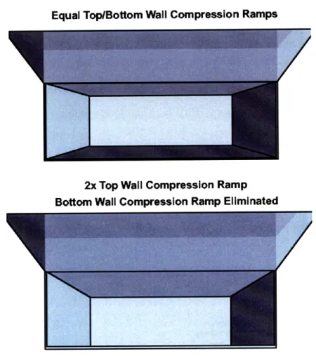
Figure 3-3: Internal Compression System Design

Figure 3-3 illustrates the two different internal compression system layouts. Scram-jet engines employ top and/or sidewall internal compression ramps. In this study, only the top and bottom wall compression ramps were modified. In the case referred to as "Ramp", both top and bottom wall compression ramps were equal. This case is illustrated at the top of Figure 3-3. The case referred to as "No Ramp" is illustrated at the bottom of this figure and employs only a top wall compression ramp. Therefore, the top wall ramp was increased by a factor of two to maintain a constant combustor inlet area.

3.1.1

Aerodynamic Performance

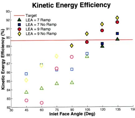
A total of 28 flow simulations were performed (every combination of leading edge angle, inlet face angle, and internal compression ramp layout). Then, the total pressure ratio and kinetic energy efficiency were used as figures of merit to guage the aerodynamic performance of each configuration. Furthermore, two constraints were imposed. Since scramjet engines require supersonic flow throughout, the first constraint required the combustor inlet Mach number to be greater than one. The second is a static tem-perature constraint. As stated in Section 1.2.2, a typical maximum combustor inlet temperature for scramjet engines is 1670 K. Therefore, combustor inlet temperatures below this limit were required. Results from the 28 cases are illustrated in Figures 3-4 and 3-5. The markers on the plot that are not filled represent those cases where one or both of the constraints were violated. Furthermore, the target total pressure ratio and target kinetic energy efficiency were computed using the combustor inlet model-ing equations given in Section 1.2.2 with an assumed compression system efficiency of

r/c = 80%.

Total Pressure Ratio

0.11 Target 0.1 A LEA = 7 Ramp U LEA=7 No Ramp 0.09 0 LEA =9 Ramp 0 LEA = 9 No Ramp

c

• .2 0.08 0.07 -, 0.06 0.05 - 0.04 0.03 0.02 0.01 3( 0 A -O O 0 45 60 75 90 105 120 135 150

Inlet Face Angle (Deg)

Kinetic Energy Efficiency

U o o y: LU o o uJ 0)

Inlet Face Angle (Deg)

Figure 3-5: Kinetic Energy Efficiency Design Comparison

Some trends are apparent in these two plots. Firstly, fixing the leading edge angle and internal ramp layout, pressure ratio and efficiency improve with increasing inlet face angle when IFA > 75'. This is likely due to the fact that the inlet capture area increases as the bottom inlet lip extends more forward. As more high pressure air is captured by the inlet, performance improves. Similarly, the hierarchy of results are

fairly consistent for IFA > 750. In other words, the LEA = 90 configurations are consistently better than LEA = 70 for IFA > 750. This is consistent with oblique

shock wave theory, wherein larger LEAs produce stronger shocks that increase the pressure and density of air behind the shock. This too increases the inlet capture area, because the higher the air density is, the more air that can fit through a given inlet geometry. One caveat is that a stronger shock produces a greater entropy and static temperature rise. Therefore, a trade-off must be performed to determine the point at which increasing the ramp angle (and shock strength) becomes detrimental.

A comparison of the Ramp and No Ramp configurations with LEA = 7' does not show a strongly correlated result from which to draw conclusions. However, the

LEA = 9' configurations show a strong correlation. For example, the No Ramp cases consistently outperform the Ramp cases. This is likely due to two effects: (i) a stronger expansion fan on the top internal surface and (ii) a stronger shock on the bottom internal surface. First, the internal top wall ramp angle is smaller for the Ramp configurations. Therefore, the transition from the external 250 ramp to the internal ramp produces a stronger expansion fan in the Ramp configurations. This stronger expansion is detrimental. Second, the bottom internal ramp increases the turning angle of the flow as compared to the No Ramp cases. This increases the shock wave strength, and consequently increases the entropy and static temperature rise across the shock. This is also detrimental. Therefore, the No Ramp case produces a weaker expansion on the top internal surface and a weaker shock on the bottom internal surface, resulting in consistently better performance. It should be noted that complex 3D interactions are also taking place. For instance, the interactions taking place between sidewall and top/bottom wall compression are difficult to envision. This is an excellent reason why simulation is worthwhile. Furthermore, some of the ambiguities seen in the results are probably due to these complicated 3D interactions that are difficult to interpret.

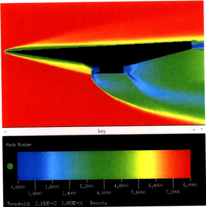
Flow visualizations of Mach number, density, and pressure were generated using Visual3 to corroborate some of the assertions made above. The best and worst case were chosen based on Figures 3-4 and 3-5 (IFA = 135°/LEA = 90_{/No Ramp and}

IFA = 600_{/LEA = 9}0_{/Ramp). Figure 3-6 reveals a couple inferiorities with this}

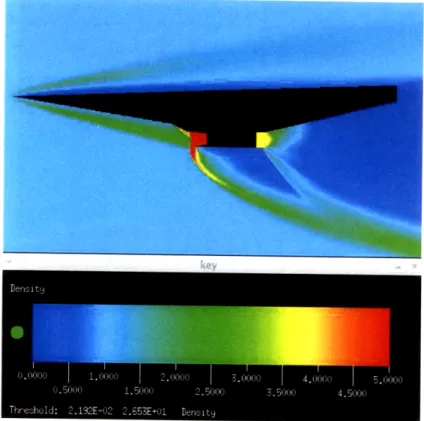
particular configuration. For instance, the Mach number at the combustor inlet is subsonic. Furthermore, the inlet face angle is too shallow and a significant amount of the air compressed by the leading edge shock is diverted beneath the engine (this is termed spillage). On the contrary, Figure 3-7 illustrates that the leading edge shock impinges on the bottom lip of the inlet. Therefore, the inlet captures most of the air compressed by the shock with very little spillage. Furthermore, the Mach number at

Figure 3-6: Mach Number Visualization for IFA = 600 LEA = 9' w/Ramp

Figure 3-8: Density Visualization for IFA = 600 LEA = 90 w/Ramp

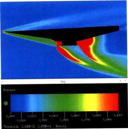
Figure 3-10: Pressure Visualization for IFA = 60' LEA = 90 w/Ramp

Figure 3-11: Pressure Visualization for IFA = 1350 LEA = 90 w/out Ramp

the combustor inlet is supersonic as required. The density plots given in Figures 3-8 and 3-9 and pressure plots given in Figures 3-10 and 3-11 tell a similar story.

3.1.2

RCS Performance

-9 -10 -11 -12 -13 -14 -15 -1; -1 -2(

Median RCS

Target A LEA= 7 Ramp N LEA =7 No Ramp * LEA = 9 Ramp LEA = 9 No Ramp O 6 7 8 -75 90 105 120 135

Inlet Face Angle (Deg)

Figure 3-12: Median RCS Design Comparison

Based on Figures 3-4 and 3-5, only 11 of the 28 configurations satisfied the com-bustor inlet Mach number and temperature constraints. Therefore, the RCS signature prediction was limited to these 11. Figure 3-12 gives the median RCS values for each of these configurations. The top three candidate aircraft configurations in terms of aerodynamics were also the top three in terms of their median RCS. ISAR images were generated for four of these configurations to compare the affect changes to LEA and ICRL had on RCS. Figure 3-15 compares the two LEA configurations for an IFA of 135'. Based on Figure 3-15, it appears that the 70 LEA case deflects more of the incident radar energy into the engine cavity. Due to the effect of ducting discussed