Adiabatic thermal Child-Langmuir flow

(1)

Adiabatic Thermal Child-Langmuir Flow

by Rachel V. Mok

B.S., Mechanical Engineering, Purdue University Calumet (2011) Submitted to the Department of Mechanical Engineering in partial fulfillment of the requirements for the degree of

Masters of Science in Mechanical Engineering MASSACHUSETTS INSTTE OF TECHNOLOGY

at the

_JUN

_{2 5 21}

MASSACHUSETTS INSTITUTE OF TECHNOLOGY

-L BRARIES

June 2013

A uth or ... I ... .... .. ... Department of Mechanical Engineering

May 10, 2013

Certified by ... ... Triantaphyllos R. Akylas Professor of Mechanical Engineering Thesis Supervisor

C ertified by ... C hiping Chen Chiping Chen Principal Research Scientist Thesis Superv or

A ccepted by ... ... David E. Hardt Chairman, Department Committee on Graduate Theses

(2)

(3)

Adiabatic Thermal Child-Langmuir Flow

by Rachel V. Mok

Submitted to the Department of Mechanical Engineering on May 10, 2013, in partial fulfillment of the

requirements for the degree of

Masters of Science in Mechanical Engineering

Abstract

A simulation model is presented for the verification of the recently developed steady-state one-dimensional adiabatic thermal Child-Langmuir flow theory. In this theory, a self-consistent Poisson equation is developed through the use of the fluid-Maxwell equations and an adiabatic equation of state. The adiabatic equation of state is also a statement of normalized rms thermal emittance conservation. Solving the self-consistent Poisson equation with the appropriate boundary conditions yields the current density, electrostatic potential, fluid velocity, equilibrium density, temperature, and pressure profiles at a given cathode temperature.

A one-dimensional simulation model has been developed. It consists of the initial

loading, the charged-sheet model algorithm, and the post-processing of the results. Great care has been taken in the initial loading of the beam, with the beam loaded as close to the equilibrium values as possible. Because there is no known solution for the interface problem between the quantum mechanical flow of electrons inside the solid material and the classical flow of electrons in the cathode vacuum, a reinjection scheme is proposed in which the initial phase space near the cathode be maintained throughout the simulation.

Three one-dimensional beams are simulated at dimensionless cathode temperatures of 0.1, 0.01, and 0.001. Great success is achieved at validating the theory at the dimensionless cathode temperature of 0.1. The simulation results for the dimensionless cathode temperature of 0.01 and 0.001 cases are consistent with the theoretical prediction. Because of the good

agreement between the simulation and theory, the use of the adiabatic equation of state is justified.

A strategy to extend the one-dimensional adiabatic thermal Child-Langmuir theory into two-dimensions is presented. Because two-dimensional adiabatic equation(s) of state are currently unknown, a two-dimensional simulation is used to both investigate and help formulate the adiabatic equation(s) of state.

(4)

A two-dimensional simulation model has been developed to simulate flows in a Pierce gun slab geometry. The two-dimensional simulation consists of the meshing of the domain, the initial loading, the particle-in-cell algorithm, and the post-processing of the results. An estimate on the two-dimensional form of the equilibrium density is used to initially load the beam. Like the one-dimensional case, the proposed particle boundary condition for the two-dimensional simulation is that the initial phase space near the cathode be preserved throughout the simulation. Preliminary results from the two-dimensional simulation model are presented.

Thesis Supervisor: Triantaphyllos R. Akylas Title: Professor of Mechanical Engineering Thesis Supervisor: Chiping Chen

(5)

Acknowledgements

This thesis would not have been possible without the help of many, many people. I would first like to thank my advisors Dr. Triantaphyllos R. Akylas and Dr. Chiping Chen. This work is completely a result of their guidance, great patience, insights, and support. I have gained much under their combined tutelage.

Thanks must also be given to MIT undergraduate researchers, Adrian Jimenez-Galindo, Kevin B. Burdge, Tenzin Rabga, and Trung V. Phan for the their assistance in the development of the one-dimensional simulation code.

Thank you to the faculty at MIT for greatly expanding my knowledge. Never before have I felt such accelerated growth in so many aspects of my life.

I would also like to thank the Engineering faculty and support staff at Purdue University Calumet for their belief and confidence in me during a time when I filled with self-doubt. I would like to especially thank Dr. Chenn Zhou, Dr. Yulin Kin, and Krasimir Zahariev for their support and guidance in my educational pursuits.

Thanks also go to all of the friends I have made here in Boston. Without their friendship and support, I would have never made it through this experience.

Finally, special thanks go to my family. My parents' unwavering love and support has been such a blessing in my life and has seen me through all the good and challenging times in my life. My brothers make life fun (most of the time). Each of my family members has

(6)

influenced me by their individual examples of love, strength, faith, perseverance, and openness. I know that I would have never become the person I am today without my family.

This work was supported in part by the United States Department of Energy, Grant No. DE-FG02-95ER40919, Grant No. DE-FG02-05ER54836, and Grant No. DE-FG02-13ER41966.

(7)

List of Figures

Figure 1-1: Theoretical and measured transverse normalized emittances for the thermionic electron gun designed for the x-ray free electron laser project at Spring-8 [12]... 23 Figure 2-1: Schematic of steady-state ID charged particle flow between two infinite plates... 28 Figure 2-2: Axial variation of the normalized electrostatic potential with space charge and

w ithout space charge... 31 Figure 2-3: Illustration of an injector with Pierce-type electrodes in a 2D slab geometry... 32 Figure 2-4: Derivation of Pierce-type electrode shapes. (a) Planar gun with a beam of infinite

width. (b) Planar gun with a beam restricted to x!5 0. In other words, the only region with electron s is x 5 0 ... 33 Figure 2-5: Plot of various normalized equipotential lines,

#

/ (Dd , _{for a Pierce-type electrode}

gun. The beam has a normalized half beam width of 0.25. Outside of the beam (x / d > 0.25 and x / d <-0.25), the normalized equipotentials are given by Eq. (2.2.3); inside the beam

(-0.25 x / d:5 0.25 ), the equipotentials are given by Eq. (2.1.8). ... 35 Figure 3-1: Schematic of steady-state ID ATCL flow between two infinite plates... 38 Figure 3-2: Evaluated dimensionless electrostatic potential distributions at the following

dimensionless cathode temperatures: T, =0.1, 0.01, 0.001 with

J= 2.6055, 1.4886, 1.1526, respectively. As a comparison, the cold-fluid solution at

(12)

Figure 3-3: Plots of the following normalized theoretical curves: (a) electrostatic potential, (b) electric field, (c) velocity, (d) equilibrium density, (e) temperature, and (f) pressure at the dimensionless cathode temperatures of T =0.1, , =0.01, and T, =0.001. As a

comparison, the cold-fluid theoretical curves, for which T, =0, are also shown... 44 Figure 3-4: 1D simulation model. The simulation loop, which implements the charged-sheet

model algorithm, consists of an electric field solver, a leapfrog scheme, and a reinjection sch em e... 4 7 Figure 3-5: Charged sheet with surface charge density a ... 51 Figure 3-6: Schematic of three charge sheets in the interelectrode space. (a) depicts the ordering

of the sheets and sources of the total electric field in each region in between the charge sheets. (b) illustrates the total electric field and the definitions of E, and SE . ... 52 Figure 3-7: Phase space of T = 0.1 at (a) t =0 and (b) t =

I.

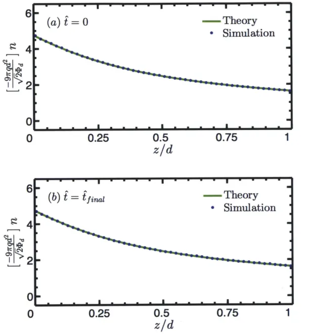
. The green line represents the

theoretical fluid velocity. ... 62 Figure 3-8: Comparison between the theoretical and simulated variation of n throughout the

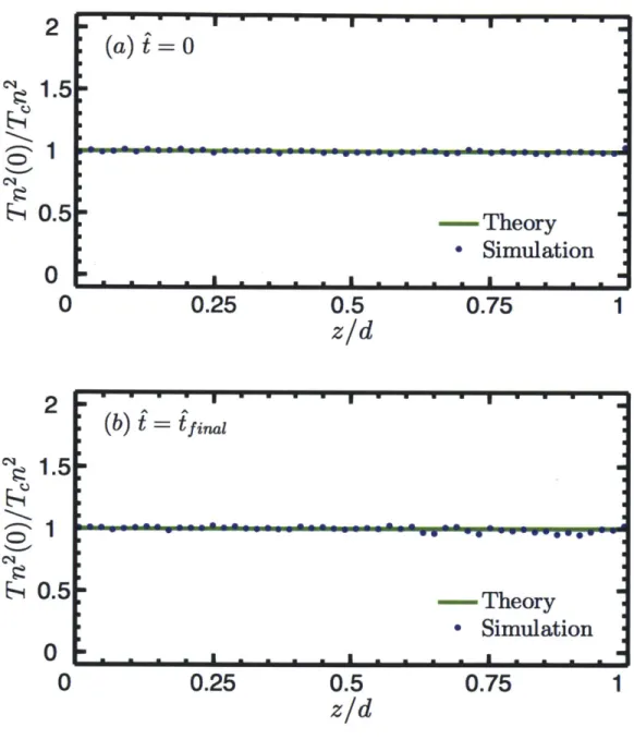
beam with Te =0.1 at (a) ?=0 and (b) = f ... 63 Figure 3-9: Comparison between the theoretical and simulated variation of Tn2 (0)/Tn2

throughout the beam with T = 0.1 at (a) t= 0 and (b) t= t, ... 64 Figure 3-10: Phase space of T, = 0.01 at (a)

i

= 0 and (b) ^ =

ifj

.The green line represents the theoretical fluid velocity ... 66 Figure 3-11: Comparison between the theoretical and simulated variation of n throughout the

(13)

Figure 3-12: Comparison between the theoretical and simulated variation of Tn2 _(0)/Tn 2 throughout the beam with T, = 0.01 at (a) ?=0 and (b)= f,...68

Figure 3-13: Phase space of T = 0.001 at (a) t =0 and (b) f =

ifj,.

The green line represents the theoretical fluid velocity. ... 70 Figure 3-14: Comparison between the theoretical and simulated variation of n throughout the

beam with T = 0.001 at (a) t= o and (b) = fi,, . ... 71 Figure 3-15: Comparison between the theoretical and simulated variation of Tn2_(0)/Tn2

throughout the beam with T, =0.001 at (a) i=0 and (b) i= ... 72 Figure 4-1: Schematic of steady-state 2D ATCL flow between two axisymmetric plates. Note

that the plates shown are just a depiction. The shapes of the plates are not limited to the geometry depicted in the figure. The only constraint applied to the plates is that they be ax isy m m etric... 76 Figure 4-2: 2D computer simulation schematic. The cathode surface is held at a constant

electrostatic potential of 0, and the anode surface is held at a constant electrostatic potential of <D. A Neumann boundary condition is applied to both the left and right sides... 78 Figure 4-3: 2D simulation model. The simulation loop, which implements the PIC algorithm,

consists of a weighting scheme from the macroparticles to the grid, a field solver, a

weighting scheme from the grid to the macroparticles, a leapfrog scheme, and a reinjection sch em e... 8 1 Figure 4-4: Mesh of simulation boundary for Ai = 0.25 and A = 0.1. The grey line shows the

original simulation boundary using the Pierce gun solution. The blue line is the staircase approximation of the simulation boundary, which defines the boundary used in the

(14)

computer simulation. The pink dots are the interior grid points. As observed in the figure, the mesh is refined in the z direction in Region I... 82 Figure 4-5: Plot of ^(i,2) using Eq. (4.2.23) for T, = 0.001 and b=0.25... 85

Figure 4-6: Loading parameters diagram. The red box shown is the loading box where loading algorithm is implemented. Although the loading box extends outside of the simulation boundary shown by the blue line, the estimated equilibrium density, Eq. (4.2.23), decays quickly to zero for T, = 0.001 and

sb

= 0.25 ... 87 Figure 4-7: PIC area weighting technique in two dimensions for a Cartesian coordinate system.

The fraction of the subdivided areas over the total area A = AM is used to weight the dimensionless charge of the macroparticle, which is assigned to the opposing corner of the cell. For example, the red area is assigned to the red grid point, the blue area to the blue grid p oint, etc... 9 0 Figure 4-8: The 5-point stencil for the Laplacian about the point (i,

j)...

92 Figure 4-9: Diagram of the example problem... 94 Figure 4-10: Numbering of the unknowns for a mesh with AI = 0.25 and W = 0.05 for

0 2 0.2 and W = 0.1 for ^ > 0.2. The unknowns are the electrostatic potential at the interior grid points... . 96 Figure 4-11: Sparsity pattern of matrix A. There are 655 nonzero elements... 97 Figure 4-12: 9^ vs. - phase space at (a) i=0 and (b)

i

=

?fi. The green line represents the ID

theoretical fluid velocity... 102 Figure 4-13: V^' vs. ^ phase space at (a)

f

=0 and (b) =

...

103

(15)

Figure 4-14: Normalized equipotential lines for the 2D slab at

I=0.

(a) shows the normalized equipotential lines for the entire geometry. (b) illustrates the normalized equipotential lines n ear th e cath ode. ... ₁₀₄ Figure 4-15: Normalized equipotential lines for the 2D slab at i = f .(a) shows the normalized

equipotential lines for the entire geometry. (b) illustrates the normalized equipotential lines n ear th e cath ode. ... 105 Figure 4-16: Comparison between the ID theoretical, 2D estimate, and simulated variation of h

along the beam axis at (a) = 0 and (b) F = fi ... 107 Figure 417: Comparison between the 2D estimate and simulated variation of n^ along the x

-axis at t= _{0 at the following locations: (a) 2= 0.1, (b) 2= 0.5, and (c) 2}= 0.9. ... 108 Figure 418: Comparison between the 2D estimate and simulated variation of n along the x

-axis over the final transit (i.e. from t = _{600 to i=1200 ) at the following locations: (a)}

Z = 0.1, (b) 2=0.5, and (c) 2=0.9. The blue dots and error bars represent the average and standard deviation of the simulation data over this time period, respectively... 109 Figure 4-19: Comparison between the theoretical and simulated variation of the dimensionless

normalized transverse emittance along the beam axis over the final transit (i.e. from

t = _{600 to t =1200 ). The blue dots and error bars represent the average and standard} deviation of the simulation data over this time period, respectively. The first two data points at the beginning of the beam have been neglected from this plot because of their high deviation from the theoretical value. ... 111

Figure A-1: Uniform grid spacing in the x direction... 117 Figure A-2: Nonuniform grid spacing in the z direction... 119

(16)

(17)

List of Tables

Table 3.1: Evaluated current densities and diode voltage at various dimensionless cathode

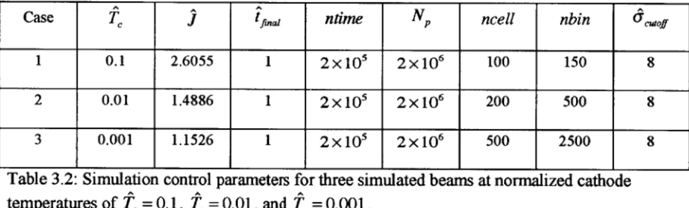
tem peratures... 46 Table 3.2: Simulation control parameters for three simulated beams at normalized cathode

temperatures of T = 0.1, T = 0.01, and

f,

=0.001... 59 Table 3.3: Derived simulation parameters for the three simulated beams... 60 Table 3.4: Maximum percent error between simulation and theoretical values for various fluid

param eters at the final tim e step. ... 60 Table 4.1: Simulation control parameters for a simulated 2D beam... 100

(18)

(19)

Chapter 1 Introduction

Adiabatic Thermal Child-Langmuir (ATCL) flows describe charged-particle flows under both a temperature and electrostatic potential bias subjected to adiabatic equation(s) of state. These

flows occur between two conducting plates and are found in the beam generation and acceleration diode of charged-particle beam systems. Recently, there is much interest and research in the development of beams with higher brightness, which is characterized by low emittance and high current, because of their potential to vastly improve the performance of many charged-particle beam applications [1, 2]. However, due to an incomplete understanding of beams in this regime, current designs experience emittance growth. Therefore, by gaining a better understanding of these flows the design of the future charged-particle beam applications may be greatly improved.

Two theoretical descriptions of non-neutral plasmas, of which charge-particle beams are a part, are the macroscopic fluid description and the kinetic description. A majority of plasma phenomena can be described using the macroscopic fluid description, which utilizes the traditional laws of conservation used in fluid mechanics, namely, the continuity equation and equation of motion for a fluid, combined with Maxwell's equations to find a self-consistent solution for the evolution of the fields and motions in the plasma from a macroscopic standpoint

(20)

certain plasma phenomena, such as Landau damping, that are unexplainable using the

macroscopic fluid description. The kinetic description utilizes the Vlasov-Maxwell equations to find the self-consistent evolution of the average electric and magnetic fields and one-particle distribution function [3]. In this thesis, the macroscopic fluid description is used and

computational simulations are performed to verify the theoretical predictions and provide insight for theoretical models.

Due to the infrequent occurrence of collisions in plasmas [4], collisions will not be considered in this thesis.

An important tool to utilize when studying plasmas is computational simulation.

Although simulations of the past could only capture the essence of plasma behavior, nowadays, with the advancement of computational capabilities, simulations can describe nearly all of the details of plasma behavior. In general, charged-particle simulations find the electric and magnetic fields from the particles' charge and current densities by solving the Maxwell

equations. Then, the classical equation of motion is used to determine the subsequent positions of charged particles [5].

The organization of this thesis is as follows. In Chapter 1, common examples of the applications of charged-particle beams are briefly discussed. In addition, recent experimental results from a state-of-the-art dc thermionic electron gun, which provides the main motivation for this research, are discussed. Chapter 1 closes with a review of two important measures of determining the quality of the beam, emittance and brightness. In Chapter 2, important background materials relevant to this work are reviewed. In particular, the known analytical results for ATCL flows in the zero temperature limit for both the one-dimensional (ID) and two-dimensional (2D) case are reviewed. In Chapter 3, the recently developed theory of ID ATCL

(21)

flows is reviewed. The ID simulation model is presented, and simulation results from three illustrative cases discussed. These results provide validation to the theory. In Chapter 4, the approach to generalize the ATCL flow theory from ID to 2D is given. The 2D simulation model is presented, and preliminary simulation results are provided. In Chapter 5, concluding remarks and directions of future work are discussed.

1.1 Motivation

Motivation for studying ATCL flows come from the shear number of charged-particle

applications and recent experimental results. By gaining a better understanding of ATCL flows, the performance of many of charged-particle beam applications may be greatly improved. In addition, experimental results from a state-of-the-art dc thermionic electron gun show a discrepancy between the measured and theoretical transverse emittances despite vast design improvements in the beam generation system. We wish to understand the causes of this discrepancy so that the designs of future beam generation systems may be improved.

1.1.1 Applications

There are many applications of high-brightness charged-particle beams, many of which are related to scientific research [2]. Two examples of charged-particle beams applications are free electron lasers (FELs) and high-energy colliders.

The main difference between a free electron laser and a traditional optical laser is that the lasing medium is from unbounded or free electrons. (Traditionally, the lasing medium of an optical laser is from electrons bound to an atom.) Therefore, because the electrons used in the FEL are unbounded, a wide range of wavelengths of the output beam can be realized through adjusting the accelerator energy and undulator parameters. The source of electrons is first

(22)

accelerated in an electron injector to near the speed of light. The electrons then move through the undulator, which comprises of a series of magnets with alternating north and south poles. The generated magnetic field forces the electrons to oscillate back and forth such that they emit light of a specific wavelength. Currently, x-ray FEL facilities are constructed or under development in the United States, Japan, and Germany. Experiments at these facilities allow the investigation of

previously unrealized areas of scientific research such as the structure of biomolecules and extreme states of matter. Furthermore, the U.S. Navy is looking into using these lasers as a defensive weapon to protect against land and air threats [6-9].

High-energy colliders are used to advance the field of particle physics, which is the study of the fundamental constituents of matter. With high-energy colliders, particle physicists hope to answer questions about the existence of extra dimensions, the postulation of unified forces at high energies, dark matter, supersymmetry, subatomic particles, antimatter, and Higgs boson particle. The largest particle accelerator to date is the Large Hadron Collider (LHC) at the European Center for Nuclear Research (CERN) in Geneva, Switzerland. At the LHC, which has

a circumference of approximately 27 km, two proton-proton beams traveling in opposite directions collide at energies of 14 TeV at four different locations around the accelerator ring [10]. Prior to the discovery of the Higgs bosons, electron-positron collider, the International Linear Collider (ILC), was proposed which would have operated at the same energies as the LHC but provide higher precision results. The design of the ILC consisted of two linear accelerators, for a total length of approximately 31 km, that collide electrons and positrons at energies up to 500 GeV. Furthermore, the proposal consisted of an option to upgrade to a 50 ki,

1 TeV collider. As a result of the recent discovery of the Higgs bosons, however, there is a demand for creating factories that collide electrons with positrons at energies of 150 GeV [11].

(23)

Other applications of charged-particle beams include spallation neutron sources, high-power microwave sources, and medical accelerators and x-ray sources [1, 2].

1.1.2 Recent Experimental Results

In a state-of-the-art dc thermionic electron gun in the Spring-8 XFEL in Japan, the following innovative design techniques were utilized: small-size cathode (the 3 mm diameter cathode consisted of a single-crystal CeB6), elimination of the cathode control grid, and adiabatic bunching and acceleration. This thermionic electron gun was able to measure a fairly low beam emittance than what is traditionally measured. For example, the transverse normalized emittance of a 1 A, 500 keV, 1400 *C beam was measured to be 1.1 mm at the gun exit. As a comparison, traditional guns typically have transverse normalized emittances of approximately 30 mm. However, the theoretical transverse normalized emittance at those parameters is 0.4 mm. Shown

in Figure 1-1 are transverse emittance measurements for different currents. Note that all of the experimental results are above the theoretical prediction [12].

2 0 100% Particles E 90% Particles E E 1.5 w 0.5

Ideal C o dae Emiltare: 0.40x mm mrad

0

z

0 0.1 0.2 0.3 0.4 0.5

V(fry)2

Figure 1-1: Theoretical and measured transverse normalized emittances for the thermionic electron gun designed for the x-ray free electron laser project at Spring-8 [12].

(24)

It is this discrepancy between the theoretical and the measured emittance that motives this research. By gaining a better understanding of the behavior of these adiabatic thermal beams, a better electron gun can be designed.

1.2 Beam Quality

Two important ways to measure the quality of a charged-particle beam are emittance and

brightness. Physically, the emittance is a measure of the parallelism of a beam, and brightness is a measure of the maximum focused power flux of the beam [13].

While there are many definitions of beam emittance, the normalized root-mean-square (rms) emittance in the transverse direction defined below is most commonly used [2].

Exn'r'M = fl) _1..1

2

where

#

=v/c, y=l 1-L, c is the speed of light in a vacuum, and ex,.,defined below, is

the unnormalized rms emittance in transverse direction

Exr. = [(x2)(X2)(X x -x' ]2 (1.2.2)

where x'= d= _ and

( )

denotes that a statistical average of the quantity inside the brackets is

dz _vZ

taken over the phase space. By Liouville's Theorem, which is a statement of phase space volume conservation, the normalized rms emittance is also conserved throughout the beam length [13].

For a thermal circular electron beam, Eq. (1.2.1) can be simplified to

- rc kBT _(1.2.3)

(25)

where me is the mass of an electron, kB is the Boltzman constant, r is the cathode radius, and T is the cathode temperature.

Brightness of a continuous beam, which can be written as a function of emittance for beams that have Cartesian symmetry in the transverse directions, is most widely defined as [2,

13]

B= (1.2.4)

(26)

(27)

Chapter 2 Child-Langmuir Flows

Many charged-particle beam applications operate in the space-charge-dominated regime because beams in this regime have high brightness. This is because the equilibrium density of beams in this regime is relatively flat over the core of the beam and then drops drastically to zero in a few Debye lengths [2]. Space-charge dominated beams are often generated by a charged-particle source operating under the space-charge-limited regime where the current is restricted by the space-charge and the electric field at the emitter is zero [14]. The cold beam, in which all thermal effects are neglected, is the simplest model of the space-charge limited regime. Flows in this regime that occur in planar diodes are also known as Child-Langmuir flows [3]. The derivation of theoretical results in this regime are reviewed.

2.1 Child-Langmuir Law

In 1911, C. D. Child derived the maximum current density of a ID flow of charged particles across an extraction gap, which is the where low-energy charged particles from a source are accelerated to moderate energy levels. It is the first stage of an accelerator. Although his derivation is only applicable to a specific geometry, it nevertheless provides a good estimate for the maximum current density of a generic charged particle extractor [13].

(28)

In his derivation, Child considered a steady-state 1 D flow of charged particles between two infinite plates separated by a distance, d, as shown in Figure 2-1. At the cathode, the electrostatic potential is zero, and at the anode the electrostatic potential is cId The velocity of

the particles at the cathode is zero. Let us further assert that the charged particles are electrons, and apply the following assumptions [13, 15]:

a) The flow is non-relativistic;

b) No collisions between the charged particles;

c) The cathode provides an unlimited flux of particles which is only limited by space-charge effects; and

d) Effects of the self-generated magnetic field are negligibly small.

d

Electron

z

Cathode (#0) Anode (#= d)

Figure 2-1: Schematic of steady-state 1 D charged particle flow between two infinite plates

(29)

dv a

m--= qE= -q- (2.1.1)

dt az

In Eq. (2.1.1), E= _{is the electric field, v is the velocity of the particle, # is the}

az

electrostatic potential, and m and q are the mass and the charge of the electron, respectively. Integrating Eq. (2.1.1) results in

v(z)= q (#(z-# (0)) (2.1.2)

where use has been made of the fact that at the cathode, all particles have zero velocity. From charge conservation, J = qnv = _{constant where n is the equilibrium density. Thus,}

J

qn = V2 (2.1.3)

2q (#(Z)-# ₍₀₎₎

where use has been made of Eq. (2.1.2). Inserting this into the ID version of Poission's equation in cgs units, V2

#

= -4 iqn, results in a2- q2 _- _{C[O(z)-_()]} 112 (2.1.4) az 2 Lq(#(z)-# (0))1/ mm

where C =-4rJ _{m. The boundary conditions for Eq. (2.1.4) used to define a unique solution}

-2q

are (0) =0,

p(d)=<D

,and =0. The third boundary condition states that the electric

field is zero at the cathode. As the amount of charged particles increases in the gap, the electric field at the cathode surface reduces until it reaches zero. At this point the surface flux at the cathode reaches its maximum value, and the flow becomes space-charge-limited flow instead of source-limited flow [13]. Therefore, the zero electric field at the cathode condition is a statement

(30)

of the maximum allowable current. Integrating Eq. (2.1.4) and applying the boundary condition

= 0 results in

= 2v5

[#(z)

-(0)]" (2.1.5)

Integrating and applying the boundary condition $(0) =0 results in

(z) =

[

315z]

(2

Finally, by applying the boundary condition

#(d)

= <Dd, the maximum current density can be expressed as

.1.6)

1 -2qo 312

97c m 2

Eq. (2.1.7) can be used to obtain a dimensionless result for the electrostatic potential in the beam

I-d (2.1.8)

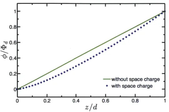
Notice that the normalized electrostatic potential with no space charge (i.e. in a vacuum) is linear, but the normalized electrostatic potential with space charge is nonlinear as shown in Figure 2-2.

(31)

z/d

Figure 2-2: Axial variation of the normalized electrostatic potential with space charge and without space charge.

2.2 Pierce Gun Solution

In 1940, J. R. Pierce was able to analytically design a space-charge dominated injector by finding the electrode shapes needed to produce a laminar beam with a uniform current density in a 2D

slab geometry. In a high-energy accelerator, the injector consists of the particle source and initial acceleration gaps. An injector with Pierce-type electrodes in a 2D slab geometry is illustrated in Figure 2-3.

(32)

z

Cathode(# = O Anode_(# =<D)

Figure 2-3: Illustration of an injector with Pierce-type electrodes in a 2D slab geometry.

To determine the electrode shapes analytically, the following assumptions were applied [13,

16]:

a) The flow is non-relativistic;

b) Effects of the self-generated magnetic field are negligibly small;

c) The emitter and collector are conducting surfaces, which maintain a potential bias. The beam exits through a grid or foil in the collector.

Consider the situation illustrated in Figure 2-4 (a). For a beam of infinite width, the variation of the electrostatic potential through the beam is given by the Child-Langmuir law, Eq. (2.1.8). However, now consider the situation illustrated in Figure 2-4 (b). There are no electrons for x >0, but there is still a flow of electrons for x! 0. For the flow of electrons in x ! 0, we

(33)

want to maintain the characteristics of an infinite width beam. In other words, in this region the resultant beam would need to be laminar, have a uniform current density, have only axial electric fields, and its electrostatic potential must vary as Eq. (2.1.8). In order to achieve this, the

boundary at x = 0 will need to satisfy the following two conditions: (1) the potential must vary as Eq. (2.1.8) at x = 0, and (2) a$/ax =0 at x = 0 because there are no transverse electric fields

for x 5 0. These two conditions can be met by using shaped electrodes.

#(0)=0=#'(0)x

+X

#(0)=0=#'(0)T

x

X

d

Emitter Collector (a) -+z

d

Emitter Collector (b)

Figure 2-4: Derivation of Pierce-type electrode shapes. (a) Planar gun with a beam of infinite width. (b) Planar gun with a beam restricted to x 0. In other words, the only region with electrons is x 0 .

To find the shape of the electrodes, the 2D Laplace equation,

3J2

_f(u)

_32fu

f = 0 (2.2.1)

ax2 az2

(34)

will need to be solved for x >0. Notice that if f(u) is an analytical function of a complex variable u = z + ix where i = -Zi , Eq. (2.2.1) is automatically satisfied for both the real and

imaginary parts of f(u) [17]. Therefore, in the vacuum region, we take $ = Re[f(u)]. Because

the potential at x = 0 is required to equal Eq. (2.1.8), the analytic function can be taken as

f(u)=<D 4/3 _ d 413 (2.2.2)

d d

Thus, the potential would be

$(x,z)=<bdRe +ix 43 (2.2.3)

It is obvious that at x = 0 , Eq. (2.2.3) satisfies condition (1), i.e. $(0,z) = CDd(z / d)4

/3. To check

if condition (2), i.e.

#/az

= 0 at x = 0, is satisfied, Eq. (2.2.3) is first expressed in polar

coordinates using

z=rcos9 , x=rsin9 (2.2.4)

where r = Vx2+ Z2 and 0 = tan-1(x/z). Eq. (2.2.3) then becomes -(

z) = Re [ 43 i4e3 = 43 cos - I (2.2.5)

[Ldd j

d

C3)

Taking the derivative with respect to x results in

a#(x,z) 4 4 2 -13 4tan-1(xz) 4 tan-'(x z)

=- D(x 2) xco -zsmn _(2.2.6)

ax 3 d3 3

Thus, at x = 0, a$(x,z)/ax =0 which satisfies condition (2). Therefore, Eq. (2.2.3) or Eq. (2.2.5) describes the electrostatic potential outside of the beam needed to maintain a laminar, uniform current density beam. The dimensionless equipotentials,

#

/ CD, for a Pierce-type

(35)

0 0.2 0.4 0.6 0.8 1 1.2 1.4 1.6 1.8

z/d

Figure 2-5: Plot of various normalized equipotential lines, / d for a Pierce-type electrode gun. The beam has a normalized half beam width of 0.25. Outside of the beam (x / d > 0.25 and

x / d <-0.25 ), the normalized equipotentials are given by Eq. (2.2.3); inside the beam

(-0.25 x /d 0.25 ), the equipotentials are given by Eq. (2.1.8).

For the cathode,

#

/Dd =0. Using Eq. (2.2.5), the cathode electrode shape would be

0= 31c /8 (2.2.7)

Therefore, the cathode is a straight line angled at 67.5* from the horizontal. For the anode,

(36)

(r/d)

4_'3_{cos(40 / 3)=1}

( The

#/<Dd=O

and

#

/CDd =1 in Figure 2-5 represent the cathode and anode electrode shapes, respectively. Thus, the modified electrode geometry has countered the beam divergence from space-charge repulsion to create a laminar beam with a uniform current density.

It is important to note that the equations that have been derived are only applicable for a planar beam. However, the electrode shapes of a cylindrical beam are close to those of a sheet beam when r, / d >>1 where r, is the radius of the beam [13].

It is also important to note that the analytical results presented in this chapter do not take thermal effects into account. In reality, however, the injector always operates at a finite

temperature. The following chapters present the development of the beam theory in which thermal effects are accounted for using the concept of adiabatic thermal beams.

(37)

Chapter 3 One-Dimensional Adiabatic Thermal

Child-Langmuir Flows

The basic theory of one-dimensional adiabatic thermal Child-Langmuir flow is reviewed. Examples of such flows are discussed. Validation of this theory is achieved through self-consistent simulations.

3.1 Theory

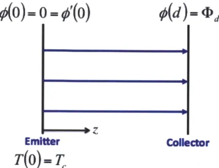
Let us consider a steady-state 1 D flow of charged particles between infinite planar conducting plates located at z = 0 and z = d subjected to a potential bias and finite temperature distribution,

as illustrated in Figure 3-1. Let us make the following assumptions:

a) The emitting plate at z = 0 is held at a constant temperature of T(0)= T;

b) The flow is space-charge dominated so that the electric field vanishes at the emitting plate;

c) The flow is nonrelativistic;

d) Effects of the self-generated magnetic field are negligibly small; and e) Effects of the fluid shear stresses are negligibly small.

(38)

#(0)=0

#'(O)

Iz

Z

Emitter

T(O)-rT

I

Collector

Figure 3-1: Schematic of steady-state 1 D ATCL flow between two infinite plates.

Under these conditions, the warm-beam fluid equations in cgs units are [18]:

mnV = -qn a ai az z aJz anV=0 = -4rqn (3.1.1) (3.1.2) (3.1.3) 0 n 3(3.1.4) p=kBnT (3.1.5)

where n, V,

#,

_{p, and T are the equilibrium density, flow velocity, electrostatic potential,}

pressure, temperature, respectively. kB is the Boltzmann constant, and m and q are, respectively, the rest mass and charge of the charged particle.

(39)

Equation (3.1.1) describes the fluid equation of motion. Equation (3.1.2) is the equation of continuity for one species. Equation (3.1.3) is Poisson's equation, which can be derived from Maxwell's equations under electrostatic conditions. Equation (3.1.4) is the ID adiabatic equation of state. Finally, Equation (3.1.5) is the ID stress tensor.

It is important to note that Eq. (3.1.4) is a statement of normalized rms thermal emittance conservation. In fact, it is a statement of entropy conservation because the propagation is

assumed to be both adiabatic (i.e. negligible heat flow) and reversible. From [19], it can be derived that in ID the square of the normalized rms thermal emittance is proportional to p /n' or

TIn2 _{. Therefore,}

T/n2 ₌_const. _(3.1.6)

along the beam.

As shown in [18], the following self-consistent Poisson equation can be derived using Eqs. (3.1.1) - (3.1.5):

32

_ 4,Ug

{- q 3 - J4W2

1/2

(3.1.7)

-qp+3kB c +[-q ~ q$ Bc c1/

subject to the following boundary conditions

(0)= 0=#0'(0) (3.1.8)

and

(d) =<Dd _(3.1.9)

where prime indicates differentiation with respect to z.

(40)

V = qp+3kB, e+

m

t

[(-~

_ q- m q, + m 6kBTc )-1/2 1/2

(3.1.10)

And at the cathode,

=3kB 1/2 mJ n(0) = 1/2 r3kBT m~c (3.1.11) (3.1.12)

3.1.1 Nondimensionalization

It is helpful to scale the relevant equations with respect to the cold beam values. The following dimensionless scales are used:

a,

- -kBT J=-, J ~z

z=-JcL d

(3.1.13)

V2 a d2, V = dV (3.1.14)

where d is the distance between the cathode and the anode; 'd is the electrostatic potential at the anode, i.e. 4D = $(0,d); T is the cathode temperature; and JcL is the Child-Langmuir cold

bemuen3 ,3/2

beam current density, i.e. Jc, = 77rd2 ( C2 ) -The dimensionless velocity, equilibrium

density, temperature, pressure, and time are defined as follows:

_ mV2 m V -

K-J

n V = -9rqd 2 vr2i(]dJ (3.1.15) (3.1.16)

(41)

=kT _(3.1.17)

9xd

p = nd2 _(3.1.18)

^d 2 1

(t g. )12t _(3.1.19)

Furthermore, the dimensionless electric field, E, is defined as

P=

R=$(3.1.20)

The dimensionless form of Poisson's equation, Eq. (3.1.3), is

V#=--n (3.1.21)

9

where use has been made of Eqs. (3.1.13), (3.1.14), and (3.1.16). Neglecting any magnetic field forces, the equation of motion for a particle is

m = qR (3.1.22)

dt2

which becomes, in dimensionless form,

d2.x

i2=

-E= $(3.1.23) where use has been made of Eqs. (3.1.13), (3.1.19), and (3.1.20).

Using Eqs. (3.1.13) and (3.1.15), the fluid velocity along the beam, Eq. (3.1.10), in dimensionless form is

(42)

In addition, using the fact that the square of the normalized rms thermal emittance, which is proportional to T / n2 in one-dimension, is conserved along the beam, the temperature profile along the beam is found to be

T= 32 2] (3.1.25)

where use has been made of Eqs. (3.1.6), (3.1.12), (3.1.16), and (3.1.19).

As shown in [18], Poisson's equation, Eq. (3.1.7), in dimensionless form becomes

a2 41 _(3.1.26)

Za-2 9 )+3]+1/26f

and the boundary conditions become

o(0)=0= 0'(0) and 0(1)=1 (3.1.27) Note that at the zero-temperature limit, i.e. T =0, Eq. (3.1.26) becomes

a2~ 4 j

(3.1.28)

which is satisfied by the solution

Z=- 3 _(3.1.29)

with J = 1. Thus, the derived Poisson's equation, Eq. (3.1.26), recovers the Child-Langmuir Law in the zero-temperature limit.

3.2 Sample Analytical Results

The ID theory discussed in §3.1 has enabled us to determine the current density and the electrostatic potential, fluid velocity, equilibrium density, temperature, and pressure profiles

(43)

given the cathode temperature for a finite-temperature nonrelativistic Child-Langmuir flow. This is accomplished by solving Eq. (3.1.26) under the boundary conditions specified in Eq. (3.1.27). Now, we present theoretical results for some illustrative normalized cathode temperatures.

1 0.751 0.5 0.25 0 0 0.25 0.5

z/d

0.75 1

Figure 3-2: Evaluated dimensionless electrostatic potential distributions at the following dimensionless cathode temperatures: T =0.1, 0.01, 0.001 with J1=2.6055, 1.4886, 1.1526, respectively. As a comparison, the cold-fluid solution at T, =0 is also shown.

Figure 3-2 shows the normalized electrostatic potential found by solving Eq. (3.1.26) with the boundary conditions in Eq. (3.1.27) for various normalized cathode temperatures. Notice that as the dimensionless cathode temperature increases, the normalized electrostatic potential becomes more and more depressed.

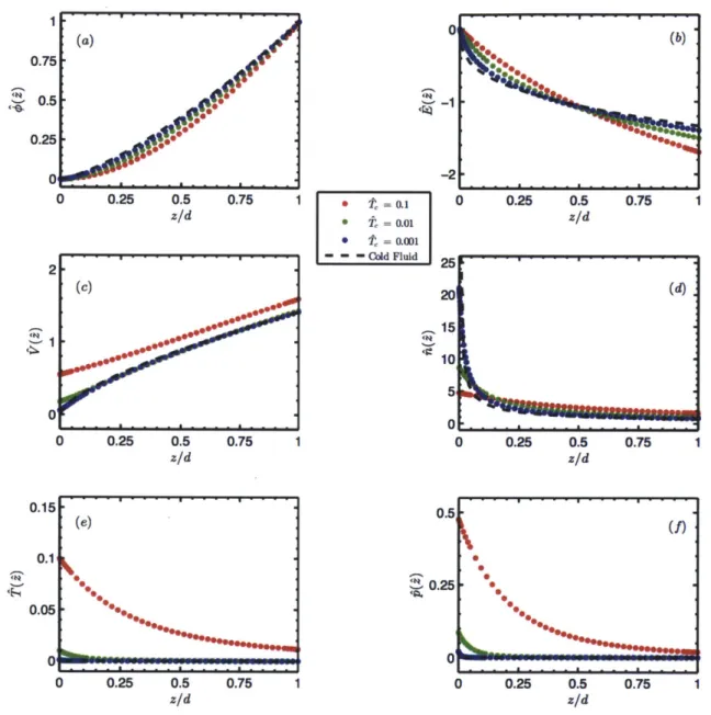
Shown in Figure 3-3 are the following normalized theoretical values: (a) electrostatic potential, (b) electric field, (c) fluid velocity, (d) equilibrium density, (e) temperature, and (f) pressure evaluated at various dimensionless cathode temperatures.

-A - 4

-eC

.

Te = 0.1 * *T = 0.01 -., = 0.001 --- Cold Fluid

(44)

'-e. 0 0.25 0.5 z/d -1 0 0.25 0.5 0.75 1 z/d I.-2 0.75 1 0 0.0 e =0.001 - - - -_{CodFluid 1 95j} 0.25 0.5 0.75 1 z/d OF-- -0 0.25 0.5 0.75 1 z/d 0.15 0.1 0.05 -- -0 0.25 0.5 0.75 z/d 0. 0.2 0 0.25 0.5 0.75 z/d 1

Figure 3-3: Plots of the following normalized theoretical curves: (a) electrostatic potential, (b) electric field, (c) velocity, (d) equilibrium density, (e) temperature, and (f) pressure at the

dimensionless cathode temperatures of T, -0.1, T = 0.01, and T = 0.001. As a comparison, the cold-fluid theoretical curves, for which T, = 0, are also shown.

-~~~~ ~ ~ -(e) e. g 5 eM 0 5 0 0 00. 1

(45)

Figure 3-3 (a) has been discussed previously. Figure 3-3 (b) describes the normalized electric field. The area bounded by this curve and the z -axis should always be equal to 1. (This will be demonstrated more formally in a subsequent section. For now, it is sufficient to know that the area is constant at all normalized cathode temperatures.) As shown in Figure 3-3 (b), the electric field does adjust itself in order to preserve the area at each T. It is interesting to note that as T decreases the rate of change in the electric field near the emitter increases. Figure 3-3 (c) illustrates the dimensionless fluid velocity. Note that at the emitter, the velocity is nonzero for the ATCL flow cases. In fact, from Eq. (3.1.11), V(O) = (3TJ .Furthermore, higher

i

results in higher velocities and a near linear profile. The dimensionless equilibrium density is shown in Figure 3-3 (d). Note that because the velocity is nonzero for ATCL flows, the equilibrium density is finite at the emitter. However, for the cold-fluid case, the velocity is zero at the emitter, resulting in an infinite equilibrium density at the emitter as shown in Figure 3-3 (d). As

T, increases, the equilibrium density becomes smoother and has a more gradual decay along the beam. Figure 3-3 (e) is a plot of the normalized temperature profile along the beam. At low

iT

's, the temperature is nearly constant throughout the beam. At high

iT's,

the temperature profile becomes more noticeable, and it is observed to decrease monotonically along the beam. Finally, Figure 3-3 (f) shows the normalized pressure variation along the beam. Because the normalized pressure is defined as the product of the dimensionless equilibrium density and temperature, pressure plot should have a form similar to Figure 3-3 (d) and Figure 3-3 (e). Like the

temperature, the pressure is nearly uniform for low Ti's. As T. increases, the profile becomes

(46)

Table 3.1: Evaluated current densities temperatures.

and diode voltage at various dimensioniess cathode

As shown in Table 3.1, ATCL flow results in a higher current density than cold-fluid Child-Langmuir flow. In fact, the current density increases as the normalized cathode temperature increases. Also shown in Table 3.1 is the corresponding diode voltage for each normalized cathode temperature with kBT, = 0.1 eV for the shown ATCL cases. Note that for

kBT =0.1 eV, a lower T corresponds to a higher diode voltage.

3.3 Simulation Model

A computer code, named One-Dimensional Adiabatic Thermal Child-Langmuir (ATCL1D), has been developed in MATLAB in order to simulate ID ATCL flows in an effort to validate the theory of ID ATCL flow. (The MATLAB code is included in Appendix C). The simulation model

and algorithms implemented in the ATCL1D code are discussed.

3.3.1 Charged-Sheet Model

The charged-sheet model is used to simulate the 1D beam. This model does not take Coulomb collisions into account [5].

kBTc J ForkB c=0.1eV, -q d CL _d 0.1 2.6055 1 0.01 1.4886 10 0.001 1.1526 100 0 1

(47)

--Loading

-I-7

Eleti Field Solve6r: r obtain electric field

a-:t

each macroparticle

I

At)

*

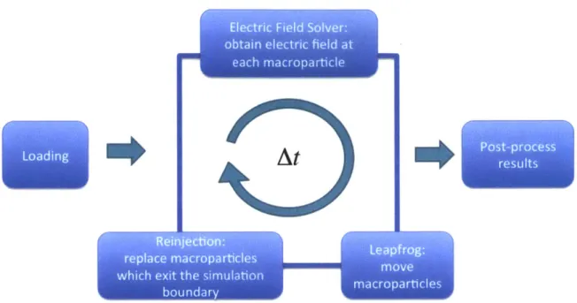
Figure 3-4: 1D simulation model. The simulation loop, which implements the charged-sheet model algorithm, consists of an electric field solver, a leapfrog scheme, and a reinjection scheme.

Figure 3-4 summarizes the computational sequence for the charged-sheet model. First, the beam is initially loaded with a set number of charged-sheets or macroparticles. In other words, all of the macroparticles are assigned an initial position and an initial velocity. Second, the simulation loop is executed. In the simulation loop, the electric field is evaluated, the macroparticles are pushed, and a reinjection scheme is implemented at each time step [5]. Finally, once the simulation loop has finished executing the set number of time steps, the results

are post-processed. In the post-processing stage, simulation values are compared to the

theoretical values and illustrative plots are obtained. In the subsequent sections, more details are given on the procedures used to execute the steps in the simulation model.

(48)

3.3.1.1 Loading

It is desirable to load the beam as close to equilibrium values as possible, achieving a so-called "quiet start." In doing so, all of the transits of the simulated beam will die out quickly; thus, the overall computational time can be decreased. To achieve a quiet start, the following strategy is employed to determine the loading of a total number of macroparticles, N,, that best represents the warm beam.

First, the total dimensionless charge of the beam is calculated from

d 25 6 di dj _di

".9,.

fffif44(3.3.1)

0

Then, the following equation is solved for the parameter, tj,,

g(?7) h((i -91)1A A

)A=

(3.3.2)

dxdy

d2 Q

where NZ is the total number of grid cells between 0 and 1 in the z direction and ddis

dd

determined from Eq. (3.3.1). Eq. (3.3.2) discretizes the theoretical equilibrium density and provides a method to find the best location in which to evaluate the equilibrium density such that the total dimensionless charge is still equal to the theoretical value. For Cell (i), the local

dimensionless charge would be

Cd

2_Q

m w((i rAe)As - 1)nAe + (3.3.3)

(49)

For the first cell, Cell (1), the number of macroparticles and residual, r, is calculated, respectively, as

d2Q

Ncel!(l) = Nearest Integer Less Than or Equal to N, ddj (3.3.4)

Pd _l) J dd2 2 r\dedj lceno> rceno>=NP d2 ~NCel>(l) (3.3.5) \# /cen(1)

For all subsequent cells, the number of macroparticles is determined by

d 2Q

NeUg, ,,,l= Nearest Integer Less Than or Equal to rceno-o + N

(d

₂

(3.3.6)

Q

Cefl~i) bd = - -1) +NP A#\ /ceu(i).J (.36

and the residual is updated according to the following equation

d 2Q

rCellO). i.1= rCell(i-1) N didd -N (3.3.7)

r -r +

(dQ

(il CeIQ)

Because there can be discrepancies using this strategy between the total loaded macroparticles and N,, a correction is implemented in which the loaded number of macroparticles are uniformly depressed or accumulated depending on if the loaded number of macroparticles is greater than or less than N,. Thus, the loaded number of macroparticles is always equal to N,.

The position of each macroparticle is determined by using a uniform random number generator for Ncell(,), with the bounds adjusted for each cell limit. To exemplify, for Cell (i), the

(50)

cell limits, a and b , that bound the uniform random number generator would be a, = (i-1) x A2

and b, = i x W.

The macroparticle's velocity is determined using a Maxwellian velocity distribution. Compared to a Gaussian distribution, the Gaussian distribution will equal the Maxwellian velocity distribution when the standard deviation is equal to

o-=kT 2

(3.3.8)

The normalized standard deviation is defined as

-1/2

m=

o m (3.3.9)

Thus, the velocity of each macroparticle is determined using a normalized Gaussian distribution random number generator with the mean equal to

V= V +31e +[q(q+6f) (3.3.10)

and the standard deviation equal to

or= T'2 (3.3.11)

where use has been made of Eqs. (3.1.24), (3.3.8), and (3.3.9). Notice that the mean of the normalized Gaussian distribution is equal to the local theoretical fluid velocity and the standard

(51)

3.3.1.2 Electric Field Solver

OF

E E

Figure 3-5: Charged sheet with surface charge density uT.

In one dimension, the macroparticles are infinite charged sheets. Let us consider the infinite charged sheet illustrated in Figure 3-5, which has surface charge density a. By planar

symmetry, the electric field emerging from a charged sheet would be perpendicular to the surface of the charged sheet and be independent of its vertical position, and for a positive surface charge density, the electric field would radiate out from the sheet. Using a Gaussian pillbox, the

magnitude of the electric field is found to be

E = I 4jra (3.3.12)

in cgs units. Notice that the electric field is not dependent on distance from the plate. In fact, the electric field is constant. Thus, for an infinite charged sheet, the electric field is constant and extends to all space [20].

Now, consider three charged sheets placed in between two conducting plates with an electrostatic potential bias as shown in Figure 3-6 (a). Let us assume that the charge sheets all have the same positive surface charge density. Thus, the magnitude of the electric field arising

(52)

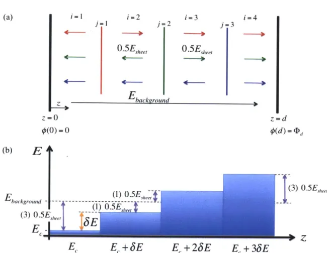
(a) i=- i-2 i-3 i-4 j-I j-2 j-3 O.5_Esee 0.5Esheet Ebackground z-0 z-d #(0)-0 _#(d)-<Ds (b)

_E

--(3) O*5Ehret E (1) ).5E0. background- --- -(3 O.5 -- (1) O5Ehe

E

.

E .

EC+

3E

EC+23E

E,+3

ME

Figure 3-6: Schematic of three charge sheets in the interelectrode space. (a) depicts the ordering of the sheets and sources of the total electric field in each region in between the charge sheets. (b) illustrates the total electric field and the definitions of Ec and SE.

from each sheet has the same constant value, 0.5E,,,,, where Esheet is equal t0 the surface charge density and any proportionality constants. For example, Esheet = 47rcr in cgs units. Because each

sheet has positive charge, the electric field of each sheet would point to the left for all regions left of the sheet and would point to the right for all regions right of the sheet. This is illustrated by the colored arrows in Figure 3-6 (a). Furthermore, an external electric field, with magnitude

Ebackground is applied throughout the region in between the conducting plates due to the potential

(53)

The total electric field for the region in between the conducting plates is the superposition of all the different electric field sources. Referencing Figure 3-6 (a), the total electric field for Region i=1 would be

E,,, = ,,,,,,,, -3 x 0.5 E,,,,,(..3

Et0,t'i1 = E,kgroufd -3X*5st (3.3.13)

For Region i =2, the total electric field would be

E,,, =2 = Ebkgru,,+ 0.5E,,, - 2 x 0.5E₅ ₁, (3.3.14)

=

)))Jkgozd- O-5Ese

= Ebk,,,, .5 E,h,, The total electric field in Region i = 3 would be

E,,,j= = Ebkgr,,,,,+ 2 x 0.5E,,, - 0.5Ehe(..5_{~ ~O~Eshed(3.3.15)}

= E,,wk,,r,,+0.-5Eh, Finally, the total electric field for Region i = 4 would be

E,,, i4 = Ekg,,,,,d+3x 0.5Eh, (3.3.16)

The total electric field in each region is illustrated in Figure 3-6 (b). Notice that total electric field is discrete and increases by a constant amount after encountering a charged sheet. An alternative way to view this problem would be to define the total electric field at Region i =1, which is the electric field at the cathode as E, and the discrete constant electric field jumps as

SE. In doing so, the electric field in each region can be described by

E,0,(i) = E, + (i-1) x SE (3.3.17) This is also shown in Figure 3-6 (b). Eq. (3.3.17) provides the basis to solve for the total electric field given a distribution of charged sheets.

Referring to Eq. (3.1.22), the electric field at each charged sheet position must be known in order to move the charged sheets forward in time. To find this quantity, the charged sheets are

(54)

first sorted according to position in ascending order. Then, Eq. (3.3.17) can be used to describe the electric field. In dimensionless form, Eq. (3.3.17) is

E(i) = E, + (i-1) x SE (3.3.18) where index i runs from 1 to (N, + 1) and corresponds to the space between the charged sheets,

E, is the dimensionless electric field at the cathode, and SE is the dimensionless magnitude of

the electric field jump from one side of the charged sheet to the other because of the presence of the charged sheet. For example, the space between the first charged sheet (at location 2^) and the

boundary ^ =0 would correspond to E(i =1) = E, and the space between the second charged

sheet (at location 2 ) and the first charged sheet (at location

z^)

would correspond to

E(i =2) = E, + SE. This is illustrated in Figure 3-6.

The quantity SE is found by considering the ID version of Eq. (3.1.21)

d _-2z0 2 _=-d do) _- d

4.Nf-=- -n (3.3.19)

d d! d4 dE 9

which can be integrated and scaled to find SE

SE = - f hdi (3.3.20)

Np 90

Note that this quantity does not change once the number of macroparticles is set. In other words,

SZ is constant throughout the simulation.

To find E , the ID version of Eq. (3.1.20) is used

$= - (3.3.21)

(55)

- d= 0=(1)- 0(0)=1I

0 _0(3.3.22)

fEd=-1

0

Notice that Eq. (3.3.22) clearly demonstrates that the area bounded by the electric field and the z

-_{axis is always a constant value independent of the normalized cathode temperature. Figure 3-3}

(b) illustrates this feature. Because the electric field is discrete, the integration can be evaluated using the following sum

E d =E x 2+

Z(L

+jx3)(+,1 - 2)+( +N, x

Z

)(1-N)

0

N-1 (3.3.23)

=E+ I (jx8Z 2,-Z-)+(N x8Z 1)(-N

j=1

where 2 is the location of the j' charged sheet. Solving for

Z,

N -1

E= - (jx SZ)(. - ,)-(NP x 8E)(i- - (3.3.24)

j=1

where use has been made of Eq. (3.3.22). Note that each time step

ZP

will change because the positions of the charged sheets will change at each time step. As a side note, recall that Ec should be zero for the space-charge-limited regime.

The electric field at the charged sheets' position is assumed to be the average of the electric fields found immediately adjacent to the charged sheet. In other words,

E()2 = [# _{(j -1E+ c+j3Ej}

(3.3.25)

Adiabatic thermal Child-Langmuir flow

Adiabatic Thermal Child-Langmuir Flow

JUN

2 5 21

-L BRARIES

Adiabatic Thermal Child-Langmuir Flow

Abstract

Acknowledgements

Contents

List of Figures

#

I.

i

ifj

ifj,.

sb

j)...

i

=

f

...

I=0.

List of Tables

f,

Chapter 1

Introduction

1.1 Motivation

1.1.1 Applications

1.1.2 Recent Experimental Results

1.2 Beam Quality

#

( )

Chapter 2

Child-Langmuir Flows

2.1 Child-Langmuir Law

#

p(d)=<D

[#(z)

[

315z]

#(d)

z/d

2.2

Pierce Gun Solution

#(0)=0=#'(0)x

#(0)=0=#'(0)T

x

X

d

d

f(u)

#/az

d

C3)

#

z/d

#

(r/d)

#/<Dd=O

#

Chapter 3

One-Dimensional Adiabatic Thermal

Child-Langmuir Flows

3.1 Theory

#(0)=0

#'(O)

Iz

Z

Emitter

T(O)-rT

Collector

#,

32

1/2

[(-~

3.1.1 Nondimensionalization

K-J

R=$(3.1.20)

3.2 Sample Analytical Results

z/d

_JUN

_{2 5 21}

_f(u)

₂

_E