Detection of a Population of Carbon-enhanced Metal-poor Stars in the Sculptor Dwarf Spheroidal Galaxy*

Detection of a Population of Carbon-enhanced

Metal-poor Stars in the Sculptor Dwarf Spheroidal Galaxy*

The MIT Faculty has made this article openly available. Please share

how this access benefits you. Your story matters.

Citation

Chiti, Anirudh et al. “Detection of a Population of Carbon-Enhanced

Metal-Poor Stars in the Sculptor Dwarf Spheroidal Galaxy.” The

Astrophysical Journal 856, 2 (April 2018): 142 © 2018 The American

Astronomical Society

As Published

http://dx.doi.org/10.3847/1538-4357/AAB663

Publisher

American Astronomical Society

Version

Final published version

Citable link

http://hdl.handle.net/1721.1/117539

Terms of Use

Article is made available in accordance with the publisher's

policy and may be subject to US copyright law. Please refer to the

publisher's site for terms of use.

Abstract

The study of the chemical abundances of metal-poor stars in dwarf galaxies provides a venue to constrain paradigms of chemical enrichment and galaxy formation. Here we present metallicity and carbon abundance measurements of 100 stars in Sculptor from medium-resolution (R ∼ 2000) spectra taken with the Magellan/ Michigan Fiber System mounted on the Magellan-Clay 6.5 m telescope at Las Campanas Observatory. We identify 24 extremely metal-poor star candidates ([Fe/H] < −3.0) and 21 carbon-enhanced metal-poor (CEMP) star candidates. Eight carbon-enhanced stars are classified with at least 2σ confidence, and five are confirmed as such with follow-up R∼ 6000 observations using the Magellan Echellette Spectrograph on the Magellan-Baade 6.5 m telescope. We measure a CEMP fraction of 36% for stars below[Fe/H] = −3.0, indicating that the prevalence of carbon-enhanced stars in Sculptor is similar to that of the halo(∼43%) after excluding likely s and CEMP-r/s stars from our sample. However, we do not detect that any CEMP stars are strongly enhanced in carbon ([C/Fe] > 1.0). The existence of a large number of CEMP stars both in the halo and in Sculptor suggests that some halo CEMP stars may have originated from accreted early analogs of dwarf galaxies.

Key words: galaxies: dwarf– galaxies: individual (Sculptor dSph) – galaxies: stellar content – stars: abundances – stars: carbon

Supporting material: machine-readable tables

1. Introduction

The oldest stars in the Milky Way contain trace amounts of elements heavier than helium(or “metals”), and measurements of their relative chemical abundances provide key constraints on the early phases of chemical evolution (e.g., McWilliam

1997; Kirby et al. 2011), galaxy formation (e.g., Freeman

& Bland-Hawthorn 2002), and the star formation history

(SFH) and initial mass function (IMF) of their birth environ-ment (e.g., Bromm & Larson 2004). Studying metal-poor

(MP) stars ([Fe/H] < −1.0, where [Fe/H] =log10(NFe NH) -

(N N )

log10 Fe H ) and, in particular, extremely metal-poor

(EMP) stars ([Fe/H] < −3.0) in the Milky Way’s dwarf satellite galaxies effectively probes the aforementioned topics due to the simpler dynamical and chemical evolution histories of dwarf galaxy systems(see Tolstoy et al.2009for a complete review). Furthermore, dwarf galaxies have innate cosmological significance, as they are hypothesized to be the surviving analogs of the potential building blocks of larger systems in hierarchical galaxy formation scenarios. Studying the most MP stars in these systems is a promising avenue to explore this intriguing potential connection.

While the specific relationship between dwarf galaxies and their ancient analogs is not entirely understood, detailed abundance studies of the most MP stars in ultra-faint dwarf galaxies and classical dwarf spheroidal (dSph) galaxies have

shown some remarkable similarities between the chemical composition of EMP stars in dSphs and in the halo of the Milky Way(Cohen & Huang 2009,2010; Kirby et al.2009; Frebel et al.2010a,2010b; Norris et al. 2010a,2010b; Simon et al.

2010; Tafelmeyer et al. 2010; Lai et al.2011; Gilmore et al.

2013; Frebel et al. 2014; Koch & Rich 2014; Roederer & Kirby2014; Jablonka et al.2015; Simon et al.2015; Ji et al.

2016). These results hint, at some level, of universality in early

chemical evolution and suggest that some of the most MP stars in the Milky Way halo could have formed in dwarf galaxies. Because of the rarity of EMP stars, further identification and study of these objects in any dwarf galaxy provides key information to further investigate these initialfindings.

Chemically characterizing members of the Sculptor dSph galaxy has provided insights on its chemical evolution and formation using high-resolution spectroscopy of red giant stars(Shetrone et al. 2003; Tolstoy et al. 2003; Geisler et al.

2005). Tolstoy et al. (2004) found evidence for two stellar

components in Sculptor, as also seen in other dSphs. More recently, Kirby et al. (2009) and the DART team (Battaglia

et al.2008; Starkenburg et al. 2010; Romano & Starkenburg

2013) used samples of ∼400–600 Sculptor stars to derive the

metallicity distribution function (MDF). Later, Kirby et al. (2011) used the MDFs of Sculptor and other dSphs to

investigate chemical evolution models. Additional modeling of Sculptor by de Boer et al. (2012) showed evidence for

extended star formation, and further modeling by Romano & Starkenburg (2013) suggested the importance of dilution and

∗_{This paper includes data gathered with the 6.5 m Magellan Telescopes}

metal removal in chemical evolution scenarios. Moreover, observations of a few individual EMP stars in Sculptor provided the first evidence that low-metallicity stars in dSphs are present and have chemical signatures matching those of EMP halo stars (Frebel et al.2010a; Tafelmeyer et al. 2010).

Further studies of the S abundances of stars in Sculptor have shown similarities with the halo at lower metallicities (Skúladóttir et al. 2015a), and studies of Zn abundances have

suggested complex nucleosynthetic origins for the element (Skúladóttir et al. 2017). Recently, work by Jablonka et al.

(2015) and Simon et al. (2015) has indicated that EMP stars in

Sculptor may have been enriched by just a handful of supernovae from the first generation of stars.

The population of stars with[Fe/H] < −2.5 in the Milky Way halo has long been known to include a large fraction enhanced in carbon (Beers et al. 1992; Rossi et al.1999; Aoki et al. 2002; Ryan 2003; Beers & Christlieb2005; Cohen et al.2005; Aoki et al. 2007; Placco et al. 2014; Frebel & Norris 2015). This

discovery led to the classification of carbon-enhanced metal-poor (CEMP) stars (MP stars with [C/Fe] > 0.7), within which exist subdivisions contingent on the enhancements of r-process and/or s-process elements. Of those, CEMP-s and CEMP-r/s stars are readily explained as the products of binary mass transfer from an asymptotic giant branch (AGB) companion (Lucatello et al.

2005; Hansen et al. 2016). However, stars that show [C/Fe]

enhancement reflecting the chemical composition of their formative gas cloud, as is thought to be the case for CEMP-r and CEMP-no stars, are the most useful in constraining theories of early chemical evolution. Proposed mechanisms behind this early carbon enhancement include“mixing and fallback” super-novae and massive rotating stars with large [C/Fe] yields, as discussed in, e.g., Norris et al.(2013).

Interestingly, the current sample of stars in Sculptor with [Fe/H] < −2.5 from Starkenburg et al. (2013), Jablonka et al.

(2015), and Simon et al. (2015) contains no CEMP stars,

contrary to expectations set by the high fraction of CEMP halo stars and earlier results that low-metallicity chemical evolution appears to be universal. Only one CEMP-no star has been previously detected in Sculptor(Skúladóttir et al.2015b), with

[Fe/H] = −2.03 and [C/Fe] ∼ 0.51, and only three CEMP-s stars are known in the galaxy out of spectroscopic samples of hundreds of stars (Lardo et al. 2016; Salgado et al. 2016).

Under the assumptions that the ancient analogs of today’s dwarf galaxies formed the Milky Way halo, one would expect that dwarf galaxies would show carbon enhancement in their oldest stellar population as well. Earlier work detected a number of carbon-strong stars in dSph galaxies, including Sculptor, but did not report individual metallicities for stars, precluding the characterization of these detected carbon-strong stars as CEMP stars (Cannon et al.1981; Frogel et al.1982; Mould et al.1982; Aaronson et al.1983; Blanco & McCarthy

1983; Richer & Westerlund 1983; Azzopardi et al. 1985,

1986). More recent searches in dSph galaxies (Lai et al.2011; Shetrone et al.2013; Starkenburg et al.2013; Kirby et al.2015; Skúladóttir et al.2015b; Susmitha et al.2017) have, however,

detected only a handful of any category of CEMP stars. To investigate this apparent dearth of true CEMP stars, or CEMP-no stars, we surveyed Sculptor with the goal of identifying EMP star candidates and robustly characterizing its MP population (T. T. Hansen et al. 2018, in preparation). We conducted follow-up observations of the most promising of these candidates to establish the low-metallicity tail of the

MDF of Sculptor and constrain the CEMP fraction in the system. In this paper, we present [Fe/H] and [C/Fe] measurements of the stars in our sample. In Section 2, we provide an overview of the target selection and observations. In Sections3and4, we outline our methods of obtaining[Fe/H] and [C/Fe] abundances for our sample. In Section 5, we discuss additional measurements and considerations that are useful in analyzing our sample. We present our results, discuss implications, and conclude in Section6.

2. Observations and Data Reduction 2.1. Target Selection

Wefirst obtained low-resolution (R ≈ 700) spectroscopy of eight fields in Sculptor using the f/2 camera of the IMACS spectrograph (Dressler et al. 2011) at the Magellan-Baade

telescope at Las Campanas Observatory. Each IMACS field spans a diameter of 27 4, and the eightfields together produce nearly complete coverage of the upper three magnitudes of Sculptor’s red giant branch (RGB) over a 37′ × 39′area centered on the galaxy, which approximately corresponds to complete coverage out to∼2 times the core radius of Sculptor (Battaglia2007). The IMACS observations were taken with a

narrowband CaK filter attached to a 200 linesmm−1 grism. With this setup, approximately 900 stars can be observed at a time. IMACS targets were selected from the photometric catalog of Coleman et al. (2005) using a broad window

surrounding the RGB so as not to exclude stars at the extremes of the metallicity distribution. The selection limits were based on a Padova isochrone(Marigo et al.2008) passing through the

Sculptor RGB and extended from 0.37mag bluer than the isochrone to 0.19mag redder than the isochrone in V−I, down to V= 20.

We selected Sculptor stars from the IMACS spectra for more extensive spectroscopic follow-up observations. We identified a sample of low-metallicity candidates by searching for stars with the smallest CaK equivalent widths, adjusting for the color of each star according to the calibration of Beers et al. (1999). The most MP known Sculptor stars from Frebel et al.

(2010a) and Tafelmeyer et al. (2010) were independently

recovered in this data set, as were two new[Fe/H] < −3.5 stars (Simon et al. 2015). We then obtained R ∼ 4000 and 6000

optical spectra of 22 of the best candidates using the MagE spectrograph(Marshall et al.2008) at the Magellan telescopes.

The majority of the observed stars were confirmed as EMP stars, including a number with spectra dominated by carbon features.

2.2. M2FS Observations

Having confirmed the utility of the IMACS data for identifying both EMP and carbon-rich candidates in Sculptor, we set out to obtain medium-resolution spectra of a much larger number of EMP candidates. We observed two partially overlapping 29 5 diameter fields in Sculptor using the Michigan/Magellan Fiber System (M2FS; Mateo et al.2012)

on the Magellan-Clay telescope. We employed the low-resolution mode of M2FS, producing R= 2000 spectra cover-ing 3700–5700 Å for 256 fibers.

The M2FS targets were selected in two categories. First, we chose all of the EMP candidates from the IMACS sample (including those confirmed as low-metallicity and/or carbon-rich with MagE spectra). Since these candidates only occupied

about half of the M2FS fibers, we then added a magnitude-limited“bright” sample containing all stars along the Sculptor RGB brighter than V= 18.1 in field 1 and V = 18.0 in field 2 (the difference between the two reflects the number of fibers available and of bright stars in each field). This bright sample should be unbiased with respect to metallicity or carbon abundance. About 30fibers per field were devoted to blank sky positions. A few brokenfibers were not used. The first M2FS field, centered at R.A., decl. (J2000) = 00:59:26, −33:45:19, was observed for 5× 900 s on the night of 2013 November 23. The second M2FSfield, centered at 01:00:47, −33:48:39, was observed for a total of 6838 s on 2014 September 14. Figure1

shows the M2FS targets for which [Fe/H] and [C/Fe] were measured in this work on color–magnitude diagrams (CMDs) of Sculptor. We note that stars with saturated CH G-bands are circled in red in the bottom left panel of Figure1. While the most carbon-enhanced stars do appear to be biased redward of the Sculptor RGB, they are not excluded from our selection procedure.

The M2FS data were reduced using standard reduction techniques(Oyarzún et al.2016). We first bias-subtracted each

of the four amplifiers and merged the data. We then extracted 2D spectra of all thefibers by using the spectroscopic flats to

trace the location of science spectra on the CCD,flattened the science data, and took the inverse variance-weighted average along the cross-dispersion axis of each science spectrum to extract a 1D spectrum.

We computed wavelength solutions using spectra of HgArNeXe and ThAr calibration arc lamps. The typical dispersion of our wavelength solution was ∼0.10 Å, which we derived byfitting third-degree polynomials to the calibra-tion lamp spectra for the 2013 data. We derived the wavelength solution for the 2014 data by fitting third-degree Legendre polynomials. We performed the sky subtraction by fitting a fourth-order b-spline to the spectra of ∼10 sky fibers on the CCD andfitting a third-order polynomial to the dependence of these spectra on the cross-dispersion direction of the CCD(e.g., the location of the fiber’s output on the CCD). We then subtracted the predicted sky model at the location of each science spectrum on the CCD and extractedfinal 1D spectra.

2.3. Follow-up MagE Observations

Motivated by the number of EMP and CEMP candidates from the M2FS data, we observed an additional 10 Sculptor stars using the MagE spectrograph on the Magellan-Baade

Figure 1.CMDs of Sculptor from Coleman et al.(2005). The M2FS targets for which [Fe/H] and [C/Fe] are computed are overplotted. Top left: [Fe/H] of stars on

the RGB of Sculptor that were selected as the most MP candidates. Top right:[Fe/H] of bright stars that were selected to fill available fibers. Much of the bright-star sample was excluded from this work(see Section3.3). Bottom left: [C/Fe] of stars on the RGB of Sculptor that were selected to be MP. Stars with saturated G-bands

telescope in 2016 September. This brought the total number of Sculptor stars observed with MagE to 31 stars, as one star had already been observed as part of the original 22 star sample(see Section 2.1). Five of these 10 stars showed strong carbon

features in their M2FS spectra. Anotherfive were not seen to be as carbon-enhanced from their M2FS spectra, but we chose to observe them due to their similar stellar parameters to the strongly carbon-enhanced stars. These 10 stars were analyzed to corroborate our M2FS carbon measurements. We also observed the halo CEMP-r/s star CS29497-034 for reference purposes. Five stars(four CEMP candidates and CS29497-034) were observed with the 0 7 slit (R ∼ 6000), which granted sufficient resolution to resolve barium lines at 4554, 4934, 5853, 6141, and 6496Å. The remaining stars were observed with the 1 0 slit (R ∼ 4000). The MagE spectra were reduced using the Carnegie Python pipeline described by Kelson (2003). With these observations, we confirmed the CEMP and

regular MP nature of our candidates, as suggested by the M2FS observations.

3. Metallicity Measurements

We used established calibrations of two spectral line indices to measure[Fe/H] from the M2FS spectra. The first such index is the KP index, a measure of the equivalent width of the CaII

K line at 3933.7Å. The second index is the LACF index, a line index derived from applying the autocorrelation function (ACF) to the wavelength range 4000–4285 Å, which is chosen due to the presence of many weak metal lines. Both line indices, along with the nature of their calibration to [Fe/H] values, are thoroughly discussed by Beers et al. (1999), and

their implementation in this work is detailed in this subsection.

3.1. Membership Selection

We measured radial velocities for each star primarily to exclude nonmembers of Sculptor. Radial velocities were measured by cross-correlating the spectrum of each star with a rest-frame spectrum of the MP giant HD122563. Wavelength calibration for spectra obtained in 2013 was carried out using a ThAr lamp, resulting in a well-calibrated range from 3900 to 5500Å. For the cross-correlation, we used this full range to determine velocities. However, spectra obtained in 2014 had associated HgArNeXe arc lamp frames taken, which provided fewer usable reference lines. It was found that cross-correlating over only the Hβ line (4830–4890 Å) gave the most precise (∼10 km s−1_{) velocity measurements for these spectra.}

More-over, velocities obtained from the M2FS fiber observations in 2014 had to be adjusted to ensure that the mean velocity of the stars was centered on the velocity of Sculptor. Accordingly, velocities measured based on fiber observations on the red CCD chip were increased by 35 km s−1. Those from the blue CCD chip observations were increased by 31 km s−1. For stars on both the 2013 and 2014 fiber plates, we used the velocity measurement from the 2013 spectrum.

We assumed that stars with velocities within 35 km s−1of the systemic velocity of Sculptor were members. This threshold corresponded to roughly 2.5σ of our distribution of velocities after excluding outliers. We found that applying this member-ship criterion recovered known members of Sculptor from Kirby et al.(2009) and Walker et al. (2009). Using this criterion, we

excluded four stars in our sample that would otherwise have been part of this data set.

3.2. Stellar Parameters

We derive initial B–V color, Teff, andlogg estimates of

stars in our IMACS sample by transforming V- and I-band photometry from Coleman et al. (2005) using a 12 Gyr,

[Fe/H] = −2.0 Dartmouth isochrone (Dotter et al. 2008).

After a first-pass measurement of [Fe/H] with this initial B–V estimate (see Section 3), we iteratively update the

metallicity of the isochrone and rederive parameters until convergence. Before any measurement of [Fe/H], the spectrum was shifted so that the CaII K line was centered at 3933.7Å. This recentering was necessary, given that the wavelength calibration was not necessarily accurate around the CaII K feature, since there was only one line below 4000Å (a weak ArIIline at 3868.53Å) in our arc frames.

3.3. KP Index

The KP index is a measurement of the pseudo-equivalent width of the CaII K line at 3933.7Å. To determine final KP indices, wefirst compute the K6, K12, and K18 indices using bandwidths of Δλ = 6, 12, and 18 Å, respectively, when calculating the equivalent width of the CaII K feature (Beers et al. 1990). Table1 lists the bands of these indices. The KP index assumes the value of the K6 index when K6< 2 Å, the K12 index when K6> 2 and K12 < 5 Å, and the K18 index when K12> 5 Å.

To derive an estimate of the local continuum around the CaII

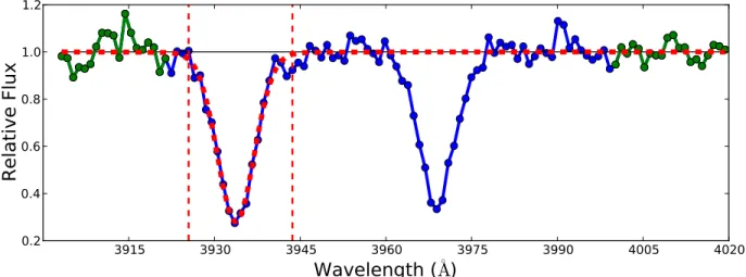
K feature, wefit a line through the red and blue sidebands listed in Table 1. We then visually inspected each continuum placement and applied a manual correction for a small subset of our sample that had an obviously badfit (e.g., due to low S/N or nearby absorption features). After continuum normal-ization, we derived estimates of the K6, K12, and K18 indices using two methods. For the first approach, we directly integrated across the line band to estimate the pseudo-equivalent width. For the second approach, we integrated over the best-fit Voigt profile to the CaII K line, as illustrated in Figure2. These two methods gave largely similar results, but the KP values from direct integration were adopted to ensure consistency with previous work involving the calibration. We derive [Fe/H] values using the KP index and B–V color as inputs to the Beers et al.(1999) calibration.

The KP index calibration from Beers et al. (1999) is only

valid for stars with B–V„1.2, meaning it can only be readily applied to 100 stars in our sample. This population largely excludes the bright-star sample, which is unbiased with respect to metallicity.

3.4. LACF Index

The LACF index measures the strength of many weak metal lines between 4000 and 4285Å (Ratnatunga & Freeman1989; Beers et al.1999). It is computed by taking the autocorrelation

Table 1 KP Line Indices(Å)

Line Blue Red Band

Index Sideband Sideband

K6 3903−3923 4000−4020 3930.7−3936.7

K12 3903−3923 4000−4020 3927.7−3939.7

of a spectrum within the aforementioned wavelength range after excising extraneous line features. The LACF index is then defined as the log of the value of the ACF at τ = 0, as defined in Equation(1) over this interval.

To ensure that we computed the LACF index in a manner consistent with that of Beers et al. (1999), we closely

reproduced their methodology. We first interpolated each spectrum using a cubic spline and rebinned in 0.5Å increments to match their calibration sample. We then excised the ranges 4091.8–4111.8 and 4166–4216 Å to remove effects from the Hδ region and CN molecular absorption, respectively. To calculate the continuum, each of the three resulting ranges were independently fit by a fourth-order polynomial, after which outliers 2σ above and 0.3σ below each fit were excluded. An acceptable continuum estimate was returned after four itera-tions of this process.

After normalizing each wavelength segment by its corresp-onding continuum estimate, we restitched the three segments together and computed the power spectrum of the resulting spectrum. We then set the high- and low-frequency compo-nents of the power spectrum to zero in order to remove the effects of high-frequency noise and continuum effects, respectively. The inverse Fourier transform of the power spectrum was taken to derive the ACF, which was then divided by the square of the mean counts in the normalized region. We finally computed the LACF index by taking the log of the resulting ACF at τ = 0.

It is important to note that an alternative expression of the ACF is

ò

where f¯ ( )l is the complex conjugate of the function f(λ). From Equation(1), it is clear that computing the LACF index,

defined as the log of the value of the ACF at τ = 0, is analogous to integrating the squared spectrum after manipulat-ing Fourier components to remove continuum and noise-related effects. This fact motivates the application of an ACF to measure line strength. As with the KP index, the LACF index is only calibrated to [Fe/H] for stars with B–V„1.2 (see discussion in Section3.3).

3.5. Comparison of Methods and Final[Fe/H] Values To ensure our measured KP and LACF indices were consistent with the existing [Fe/H] calibration, we measured them on a subset of the calibration sample in Beers et al. (1999). We found agreement in the KP indices but a

gradually increasing scatter in the LACF measurements when LACF<0, which roughly corresponds to very MP stars, stars with high effective temperatures, or stars with spectra that have low S/N. We thus chose to discard the LACF-based metallicity measurement for stars with LACF<−0.5 or when [Fe/H]KP<

−2.5. Since the LACF works best at measuring [Fe/H] in the more metal-rich regime, where weak metal lines are more prominent, this exclusion seems reasonable. We also chose to discard KP-based metallicity measurements when[Fe/H]KP>

−1.0, motivated by the failure of the KP calibration at high metallicities due to the saturation of the CaII K line. In the regime where both KP- and LACF-based metallicities are valid, we take the average of the two measurements weighted by the measurement uncertainty.

Theα-element abundance of stars in the Beers et al. (1999)

calibration is assumed to be[α/Fe] = +0.4 for [Fe/H] < −1.5 and[α/Fe] = −0.27×[Fe/H] for −1.5 < [Fe/H] < 0. Stars in Sculptor display a different trend in[α/Fe] with [Fe/H]. We account for this discrepancy by first computing an [α/H] measurement for our stars based on the aforementioned α-element trends used in the Beers et al. calibration for both the KP- and LACF-derived metallicities. We thenfit a line to a Sculptor [Fe/H] versus [α/H] trend derived from measure-ments in Kirby et al.(2009) and use this trend to compute an

[Fe/H] measurement from our [α/H] measurement for each of our Sculptor stars. This adjustment is motivated by the fact that the Beers et al.(1999) calibrations measure the strength of

α-element features and derive metallicities under the assumption of a given[α/Fe] for halo stars, which is discrepant from the trend in dwarf galaxy stars. This correction typically increased the metallicities of stars in our sample by0.1 dex, since it had no effect on stars with [Fe/H] < −3.0 and increased metalli-cities of stars with[Fe/H] = −2.5 by ∼0.1 dex.

Initial [Fe/H] uncertainties were assigned following Beers et al.(1999). To account for uncertainties in using an isochrone

to transform between V–I and B–V color, we propagated the uncertainty in our original V–I color to the final [Fe/H]

Figure 2.Spectral region around the CaIIK line(3933.7 Å) after continuum normalization. The horizontal black line depicts the continuum fit to the blue and red sidebands(green), and the vertical red dashed lines correspond to the range of integration for the KP index. The overplotted red dashed line corresponds to the best-fit Voigt profile.

measurements and added this effect in quadrature to the other uncertainties. We also propagated uncertainties in the age of the isochrone, which had negligible effects. Finally, we remeasured the metallicities after shifting the continuum by the standard errors of thefluxes in the red and blue continuum regions. The difference between the remeasured and original metallicities was added in quadrature with the other estimates of uncertainty. Typical uncertainties are∼0.25 dex.

3.6. External Validation: Comparison to Globular Cluster Members

As an external check on our metallicity measurements, we determined [Fe/H] values for cool (Teff< 5500 K) member

stars in four globular clusters (M2, M3, M13, and M15) with metallicities ranging from[Fe/H] = −2.33 to −1.5. We retrieved medium-resolution spectra of these stars from the Sloan Digital Sky Survey-III7(Eisenstein et al. 2011; Ahn et al. 2014). The

V–I colors were derived by applying an empirical color transformation following Jordi et al.(2006).

The metallicity spread among members of a globular cluster is a fraction of our measurement uncertainties, with the exception of some anomalies in M2(Yong et al.2014). Thus,

we used the offset of our[Fe/H] values of each cluster member from the average metallicity of the globular cluster to gauge the validity of our metallicity calibration. Before measuring metallicities, we recorded the mean [α/Fe] of these globular clusters from Carney (1996), Kirby et al. (2008), and Yong

et al. (2014) and corrected them for the discrepant [α/Fe]

assumption in our calibrations. As shown in Figures 3 and 4, our measurements gave largely reasonable results, with an overall[Fe/H] offset of −0.02 dex and scatter of 0.18 dex. This is consistent with our typical derived uncertainty in[Fe/H] of ∼0.25 dex.

3.7. External Validation: Comparison to Kirby et al. Kirby et al. (2009, 2010,2013) measured the metallicities

and α-abundances of a total of 391 stars in Sculptor with medium-resolution spectroscopic data from the Deep Imaging Multi-Object Spectrometer on the Keck II telescope. We found 86 stars in common with our full sample of ∼250 stars, of which 20 stars have B–V„1.2. We compare the stellar parameter measurements of all 86 stars. We find reasonable agreement in our Teffmeasurements as demonstrated by a mean

offset of DTeff =25 K and a standard deviation of σ(ΔTeff) = 137K. For log , we correct the significant offsetg

of +0.39 dex compared to the Kirby et al. sample. The mean difference in logg after this correction is 0, with a standard deviation of 0.17 dex. If we were to only consider stars with B–V„1.2, then the standard deviation would be 0.23 dex. This correction also results in agreements withlogg values of stars with high-resolution spectroscopic stellar parameters(see Table 2). We note that not applying this gravity correction

would artificially increase the carbon abundance correction we apply to take into account the evolutionary state of the star(see Placco et al.2014) and thus the number of CEMP stars in the

sample. We then compare our metallicities for the subset of stars with B–V„1.2. We find a mean offset of [Fe/H]−[Fe/H]K10≈−0.11 dex with a standard deviation

of ∼0.15 dex (excluding two outliers below B–V = 1.2, for

which we measure a lower metallicity by over ∼0.5 dex; see Figure5). Including these outliers changes the mean offset to

[Fe/H]–[Fe/H]K10≈−0.16 dex and increases the scatter to

∼0.19 dex.

Both outliers(10_8_2730 and 10_8_2788) in Figure5have low reported calcium abundances ([Ca/Fe] = −0.23 ± 0.30 and 0.05± 0.39) in Kirby et al. (2010). This could lead to a

weaker CaII K line than our assumed [α/Fe] would suggest and would cause an underestimation of the metallicity.

Figure5 also demonstrates the failure of the KP and ACF calibrations for B–V > 1.2. Accordingly, we choose to limit this work to the subset of stars in our sample with B–V„1.2.

3.8. External Validation: Comparison to High-resolution [Fe/H]

As afinal check to ensure that the KP calibration holds for EMP stars, we retrieved high-resolution spectra of four EMP Sculptor members from Simon et al. (2015).8 We smoothed these spectra to match the resolution of our medium-resolution data and degraded the S/N to 20 Å−1. We then computed the KP-derived metallicities of these stars. The results are shown in the top section of Table2and demonstrate the accuracy of KP calibration.

We also compared the KP-derived metallicities from our M2FS sample to high-resolution measurements in Jablonka et al.(2015) and Simon et al. (2015) for five stars in common to

both samples. The results are shown in the bottom section of Table2. We note a marginally higher KP-derived metallicity in most cases for the EMP stars in the M2FS data. The largest residual(11_1_4296) can reasonably be explained due to the presence of noise near the CaIIK line. Interpolating over this noise spike results in a marginally lower disagreement of +0.34 dex when compared to the high-resolution [Fe/H] measurement.

4. Carbon Abundance Measurements

To derive carbon abundances ([C/Fe]), we matched each observed spectrum to a grid of synthetic spectra closely following the methodology of Kirby et al. (2015). We

generated these using the MOOG spectrum synthesis code with an updated treatment of scattering(Sneden1973; Sobeck et al.2011) and model atmospheres from ATLAS9 (Castelli &

Kurucz 2004). We independently computed [C/Fe] using

regression relations from Rossi et al. (2005) but found that

fitting to a grid allowed accurate [C/Fe] measurements over a broader range of input parameters.

4.1. Spectrum Synthesis

Table3 lists the stellar parameters of the generated grid of synthetic spectra. We used a comprehensive line list spanning 4100–4500 Å compiled by Kirby et al. (2015). The list

comprises transitions from the Vienna Atomic Line Database (VALD; Piskunov et al.1995; Kupka et al.1999), the National

Institutes of Standards and Technology(NIST; Kramida et al.

2014), Kurucz (1992), and Jorgensen et al. (1996). We

assumed an isotope ratio of 12C/13C= 6 based on the low surface gravity (logg2.0) of most of our stars. The

α-element abundance of the grid was chosen to be +0.2 dex,

7

http://dr10.sdss3.org

8 _{The spectrum of thefifth star in that paper does not extend blueward to the}

which is the mean expected value for this sample of Sculptor members, as gleaned from measurements by Kirby et al. (2009). Each synthetic spectrum was degraded to match the

resolution of medium-resolution M2FS spectra. This grid was then used for measuring the carbon abundances reported in this paper. It should have similar inputs (e.g., line lists, model

atmospheres) to previous works on the CEMP fraction in dwarf galaxies(e.g., Kirby et al.2015) and other studies of halo stars.

This enables a fair comparison of our results with literature values.

To appropriately compare our [C/Fe] measurements with nearly all values in the literature, we generated two smaller test grids based on model atmospheres and line lists different from those in the primary grid used in our analysis. Thefirst test grid was generated using the Turbospectrum synthesis code (Alvarez & Plez 1998; Plez 2012), MARCS model

atmo-spheres (Gustafsson et al.2008), and a line list comprised of

atomic data from VALD, CH data from Masseron et al.(2014),

and CN data from Brooke et al. (2014) and Sneden et al.

(2014). The second test grid had the same inputs as the first but

was generated using MOOG to compare differences between just the two synthesis codes. Both test grids spanned 4500–4800 K in effective temperature, 1.0–2.0 dex in log g, and −4.0 to −2.5 dex in [Fe/H], which roughly covers the stellar parameters of the more MP stars in our sample.

4.2. Fitting to the Grid

Since synthetic spectra computed by MOOG are generated as normalized spectra, we normalized each spectrum. We found that iterativelyfitting a cubic spline to the observed data from 4100 to 4500Å, excluding points 5σ above and 0.1σ below in each iteration, reproduced the continuum well. After dividing

Figure 3.Histograms of the difference between our measured metallicity of each globular cluster member and the overall cluster metallicity for globular clusters M3 (top left), M13 (top right), M2 (bottom left), and M15 (bottom right).

Figure 4.Difference between our measured metallicity of each cluster member and the overall cluster metallicity as a function of B–V color. Dashed lines correspond to±0.25 dex. The mean of the distribution of residuals is −0.02, and the standard deviation is 0.18.

the observed spectrum by our continuum estimate, we found the best-fitting synthetic spectrum by varying [C/Fe].

We then implemented a χ2minimizer to match the region spanning the CH G-band (4260–4325 Å) to the synthetic grid. We measured[C/Fe] by setting the three parameters Teff, log g,

and [Fe/H] equal to the values determined from our medium-resolution M2FS measurements and letting [C/Fe] vary as a free parameter. We then interpolated between thefive [C/Fe] measurements around the best [C/Fe] value with the lowest χ2_{values to determine afinal carbon abundance. Sample fits}

are shown in Figure 6. Each [C/Fe] measurement was corrected to account for the depletion of carbon for stars on the upper RGB (Placco et al.2014). After this correction, we

find no statistically significant trend in the [C/Fe] abundances with respect to measured log g values.

To determine the uncertainty in our carbon abundance measurements, we remeasured [C/Fe] 100 times for each spectrum after varying the stellar parameters each time. For each measurement of[C/Fe], we drew values of Teff, log g, and

[Fe/H] from Gaussian distributions parameterized by the medium-resolution measurements and uncertainties of those parameters. We adopted stellar parameter uncertainties of ±150 K for Teff and ±0.15 dex for log g. Before each

measurement, the continuum was multiplied by a number drawn from a Gaussian distribution centered on one with σ = 0.01 to capture the uncertainty in continuum placement. The standard deviation of the resulting [C/Fe] measurements was taken as the total uncertainty in our measurement.

4.2.1. External Validation: Comparison to SkyMapper Sample from Jacobson et al.(2015)

We applied our framework to measure [C/Fe] values to a sample of high-resolution Magellan/MIKE spectra of MP halo stars selected from the SkyMapper survey. These spectra were degraded to match the resolution of our medium-resolution spectra and injected with Gaussian noise to bring the S/N down to 20Å−1. High-resolution[C/Fe] abundances computed by Jacobson et al. (2015) were used as reference values.

Analyzing a sample of 84 stars, we find that our [C/Fe] values differ from the high-resolution [C/Fe] values by a median value of 0.03 dex, with σ(Δ[C/Fe]) = 0.22 dex (see Figure 7). We regard this agreement as excellent, since

different normalization routines tend to produce different

[C/Fe] measurements, given the difficulty of normalizing the G-band due to ubiquitous absorption features. Furthermore, the average offset is dwarfed by the typical measurement uncertainty of ∼0.35 dex. Raising the continuum placement by 2% increases[C/Fe] by ∼0.1 dex in this sample.

4.3. External Validation: Comparison to Kirby et al.(2015) and Simon et al.(2015)

Three stars in our sample have high-resolution [C/Fe] measurements in Simon et al. (2015) with which we find

agreement, as shown in Table4. Eight stars in our sample have medium-resolution [C/Fe] measurements in Kirby et al. (2015). We find good agreement with their measurements,

except for one star for which we measure a higher[C/Fe] by 0.6 dex. If we adopt the stellar parameters provided by Kirby et al. (2015), then the discrepancy reduces to 0.33 dex. This

resulting discrepancy appears to be reasonable given the reported uncertainty in our[C/Fe] measurements of ∼0.35 dex and the low S/N of the M2FS spectrum of the star.

4.4. External Validation: Comparison to Jablonka et al.(2015) Two stars in our sample have high-resolution [C/Fe] measurements in Jablonka et al. (2015). We do not find

agreement in the [C/Fe] measurements, as our measurements are at least ∼0.8 dex higher (see Table 4). We note that

Jablonka et al. (2015) adopted log( )C=8.55 (Anders &

Grevesse1989; Grevesse & Sauval1998), which is discrepant

with thelog( )C=8.43 assumed in MOOG(Asplund et al.

2009). This can account for 0.12 dex of the total [C/Fe] offset

between the measurements.

To explore whether the rest of this discrepancy could reasonably be explained by differences in the spectrum synthesis codes, model atmospheres, or line lists, we first attempted to reproduce the synthesis shown in Jablonka et al. (2015) for star ET0381. We were able to reproduce their

synthesis using Turbospectrum, the MARCS model atmos-phere, and the Masseron line list, but we noticed a consistent offset of∼0.5 dex if we attempted to reproduce the synthesis with our adopted line list and MOOG. This total observed discrepancy between our two approaches reasonably accounts for most of the observed offset between[C/Fe] measurements, and about half of this observed ∼0.5 dex discrepancy can be

Table 2

Stellar Parameter Comparison

ID loggMR loggHR TeffMR(K) TeffHR(K) [Fe/H]KP [Fe/H]HR Δ[Fe/H] References

S1020549 1.30 1.25 4610 4702 −3.74±0.21 −3.68 −0.06 S15 Scl 6_6_402 1.67 2.00 4796 4945 −3.91±0.25 −3.53 −0.38 S15 Scl 11_1_4296 1.52 1.45 4716 4770 −3.90±0.21 −3.77 −0.13 S15 Scl 07−50 1.35 1.05 4676 4558 −3.96±0.20 −4.05 +0.09 S15 S1020549 1.29 1.25 4581 4702 −3.63±0.21 −3.68 +0.05 S15 Scl 11_1_4296 1.55 1.45 4697 4770 −3.33±0.22 −3.77 +0.44 S15 Scl 07−50 1.40 1.05 4641 4558 −3.77±0.20 −4.05 +0.28 S15 ET0381 1.19 1.17 4532 4540 −2.83±0.19 −2.83 +0.00 J15 Scl_03_059 1.10 1.10 4492 4400 −3.00±0.15 −3.20 +0.20 J15

Note.Here[Fe/H]KPis the metallicity measured by applying the KP index calibration, and[Fe/H]HRis the metallicity measured in the indicated reference paper.

Measurements labeled “MR” are medium-resolution measurements following the methodology of this paper. Top section: measurements from smoothed high-resolution spectra of stars presented in Simon et al.(2015). Bottom section: measurements from our medium-resolution M2FS spectra. Here S15 and J15 refer to

Simon et al.(2015) and Jablonka et al. (2015), respectively. The log g values in this table have been corrected by +0.39 dex to account for the measured offset with

ascribed to differences in the line lists and adopted solar abundances.

To ensure that our CEMP detections were not susceptible to differences in synthesis codes, line lists, and model atmo-spheres, we replicated our analysis for our CEMP stars using the two test grids discussed in Section 4.1. We measured [C/Fe] for the subset of stars falling within the grid. As shown in Figure 8, the discrepancies in [C/Fe] between the two synthesis codes are largely within 0.2 dex but grow larger for carbon-poor stars. Different model atmospheres and input line lists cause up to another∼0.1–0.2 dex difference. Referring to Figure 8, we note that a star such as ET0381 with a measurement of [C/Fe] ∼ −0.20 in MOOG tends to have an abundance lower by∼0.15 dex in Turbospectrum. If we apply additional offsets accounting for differences in line lists and adopted solar abundances, we recover the aforementioned offset of ∼0.50 dex. However, the classification of carbon-enhanced stars appears to be largely robust to different synthesis codes, model atmospheres, and input line lists.

4.5. Confirmation of [C/Fe] with MagE Spectra and Further Classification

Motivated by the high number of CEMP stars in the M2FS sample, we conducted follow-up observations of 10 Sculptor stars with the MagE spectrograph as outlined in Section 2.3. This sample included five strong CEMP candidates and five stars that were not as carbon-enhanced but had similar stellar parameters to thefive CEMP candidates. We also observed one halo CEMP-r/s star, CS29497-034, as a comparison.

The purpose of these observations was to apply an independent check on our overall classification scheme and to potentially derive the barium abundance of the stars to further classify them. Large Ba abundances in carbon-rich MP stars are a strong indicator of the stars belonging to the CEMP-s and CEMP-r/s classes that are generally explained as being caused by accretion from a binary companion(Hansen et al.2016). The

more metal-rich analogs are the CH-strong and Ba-strong stars (McClure & Woodsworth1990). Any of these stars have to be

excluded when computing a CEMP fraction, as their carbon enhancement does not reflect the abundance pattern in their birth environment. We indeed verified the carbon-rich nature of the five stars in our sample but found four of them to be more metal-rich stars of potentially either the CH-strong or Ba-strong class (see Section5.1). The other star was observed with the 1″ slit,

which does not provide sufficient resolution to measure barium features. The M2FS spectra of a few strong carbon-enhanced stars are shown in Figure9.

4.6. Identifying Accreting Binary Carbon-rich Stars in Our M2FS Sample

It is necessary to exclude carbon-rich stars whose source of enhancement is extrinsic (e.g., accretion from a binary companion) from our calculation of the CEMP fraction. Generally, members of this class of carbon-rich binary stars can be identified by radial velocity monitoring or by detecting a combined enhancement in s-process elements (e.g., Ba) together with carbon that would have been produced in a companion AGB star. But recent work by Yoon et al.(2016)

suggests that stars with sufficiently high absolute carbon abundance (A(C)) can already be identified as CEMP-s stars just based on the[Fe/H] and A(C) measurements, as shown in Figure10.

We can readily apply the Yoon et al. criterion to both our M2FS and MagE samples. However, for the four most carbon-enhanced stars in our MagE sample, there is a discrepancy in our carbon abundance measurements. The A(C) values derived from the MagE data suggest these stars to be clearly s-process-rich stars, while the M2FS A(C) measurements

Figure 5.Left: comparison of[Fe/H] measured by Kirby et al. (2010) and in this work for the 86 stars in both samples. Blue points correspond to stars with

B–V„1.2, and red points correspond to stars with B–V > 1.2. Right: difference between [Fe/H] measured in this work and by Kirby et al. (2015) as a function of

B–V color. The vertical line marks the cutoff, to the right of which B–V colors are not directly calibrated to [Fe/H] in Beers et al. (1999). Dashed lines indicate

±0.30 dex.

Table 3

Synthetic Spectrum Grid Stellar Parameter Range

Parameter Minimum Maximum Step

λ 4250Å 4350Å 0.01Å

Teff 3700 K 5700 K 50 K

log g 0.0 4.0 0.5

[Fe/H] −4.0 +0.2 0.2

place them on the boundary according to the Yoon et al. criterion.

The higher resolution of the MagE spectra better resolves the G-band and the C2band head and suggests that these four stars

are more carbon-enhanced than inferred from the lower-resolution M2FS spectra. In addition, renewed inspection of the CaII K line reveals the same trend; these four stars are actually more metal-rich than the KP index measurement from the M2FS data had indicated. Overall, these revisions strongly suggest that the four stars could either be CEMP-s stars(if they indeed have [Fe/H]−1.5) or belong to the class of even more metal-rich CH-strong or Ba-strong stars.

Regarding the carbon abundance discrepancy, we note that when high carbon abundances lead to strong spectral absorp-tion features (especially in cool stars), there is no region in the vicinity of the G-band (4250–4350 Å) to place the true continuum value in M2FS spectra. Thus, even accounting for this effect can still easily lead to systematically underestimating the continuum and thus the carbon abundance. These four stars all had[C/Fe]M2FS1. We thus speculate that the G-band in

the M2FS spectra begins to saturate around[C/Fe]M2FS∼ 1.

We note that the G-band in the higher-resolution MagE spectra also begins to saturate for those four stars. This is illustrated by our inability to use the G-band to recover the literature[C/Fe] measurement of CS29497-034, a star with a similar G-band depth in the MagE spectra as our Sculptor members with high[C/Fe]. Motivated by the near-saturation of the G-band for these stars, we instead determined the carbon abundances of CS29497-034 using the C2band head at 5165Å.

We used a line list compiled from Sneden et al.(2009,2016)

Figure 6.Spectral region around the G-band together with the best-fitting synthetic spectra (blue) for three example observed M2FS spectra (black). Synthetic spectra with[C/Fe] closest to the 1σ upper and lower [C/Fe] measurements are overplotted in red and green, respectively.

Figure 7.Carbon abundance measurements of MP stars from Jacobson et al. (2015) after the spectra were degraded to the same resolution as the Sculptor

M2FS spectra vs. high-resolution[C/Fe] measurements of the same stars. The median offset between the medium- and high-resolution[C/Fe] measurements is 0.03 dex, and the observed scatter is 0.22 dex.

and Masseron et al.(2014) and the MOOG synthesis code. We

measure[C/Fe] = 2.6 ± 0.1 for CS29497-034, consistent with the literature value of [C/Fe] = 2.72 (Aoki et al. 2007). We

thus use the C2band head to measure carbon abundances for

the stars observed with MagE that have a near-saturated G-band.

We find 11 stars with [C/Fe]M2FS> 1.0 and showing the

presence of a C2band head and a very strong G-band, which

we suspect to have underestimated carbon abundances. If the A(C) value of these stars were revised upward by ∼1 dex (following the results for CS29497-034 and the four stars also observed with MagE), they would clearly be members of the

ET0381 −0.18±0.34 −1.00±0.15a +0.82b J15

scl_03_059 −0.39±0.40 −1.20±0.40a _+0.81b _J15

Notes.Here S15, K15, and J15 refer to Simon et al.(2015), Kirby et al. (2015), and Jablonka et al.(2015), respectively. a

Jablonka et al.(2015) presented asymmetric uncertainties. These are the average of their asymmetric uncertainties. b

See Section4.4for a discussion of the potential causes of these discrepancies.

Figure 8. The [C/Fe] measured with Turbospectrum, the MARCS model atmospheres, and the Masseron et al.(2014) line list vs. [C/Fe] measured with

MOOG and the same inputs. Dashed lines indicate±0.2 dex offsets to guide the eye.

Figure 9.The M2FS spectra of four stars(from top: 10_7_486, 10_8_3963, 11_1_4121, and 11_1_6440) that have saturated G-bands (∼4315 Å). We measure their carbon abundance using the C2 band head at 5165Å in their corresponding MagE spectra.

Figure 10.Yoon et al. plot with the original sample of halo stars in black and our Sculptor CEMP candidates overlaid in red, cyan, and magenta points. Groups I, II, and III are represented by blue, green, and orange ellipses, respectively. Cyan points correspond to M2FS measurements of stars with saturated G-bands and lower limits on their carbon abundances and metallicities, magenta points correspond to M2FS measurements of stars with saturated G-bands but accompanying MagE carbon abundance measurements, and magenta points in Group I are MagE measurements of those stars with saturated G-bands. The majority of Group I stars are CEMP-s stars, and the majority of Group II and III stars are CEMP-no stars

class of s-process-rich stars, based on the Yoon et al. plot(see Figure 10). We thus consider these stars as s-process-rich

candidates and list our derived carbon abundances strictly as lower limits in Table 6. Table5has afinal list of the iron and carbon abundances computed for the subset of all 31 MagE spectra with B–V < 1.2. Given the ambiguity in the metallicities of the carbon-rich stars observed with MagE, we cautiously only list A(C) measurements for those stars.

5. Chemical Signatures of the MP Stellar Population of Sculptor

5.1.[Ba/Fe] Estimates from MagE Spectra and Exclusion from CEMP-no Classification

In our follow-up MagE observations (Section 2.3) of

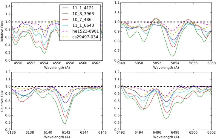
10 stars, we observed four of the five very carbon-enhanced candidates with the 0 7 slit to obtain sufficient resolution (R ∼ 6000) to also resolve barium lines at 4554, 4934, 5853, and 6141Å. We used a line list from Sneden et al. (2009,2016)

and the MOOG synthesis code to synthesize these lines and constrain [Ba/Fe].

At R∼ 6000, these four lines can be blended, e.g., with praseodymium at 5853Å, when neutron-capture element abundances are high, as in s-process-rich stars. We are able to reproduce the literature [Ba/Fe] = 2.2 measurement of

CS29497-034 when considering the depth of the centroid of the line and neglectingfitting the entire line profile. This suggests that the blending features do not significantly affect the centroid of the barium lines. In Figure11, the barium lines of the stars are overplotted with the resolution-degraded MIKE spectrum of the halo r-process star HE1523–0901 (Frebel et al. 2007), which has similar stellar parameters to the four

Sculptor stars. The barium features of the Sculptor stars are stronger than those in the reference stars CS29497-034 ([Ba/Fe] = 2.2) and HE1523–0901 ([Ba/Fe] = 1.1), suggest-ing that they are s-process-enhanced stars with[Ba/Fe] > 1.0. The centroid measurements for these stars yield high [Ba/H] values of 0.36, 0.8, −0.53, and −0.18. Taking our KP-based Fe measurements at face value, these abundances translate to [Ba/Fe] = 3.00, 3.80, 2.50, and 2.60. However, these stars show strong CH features in the vicinity of the CaIIK line in their spectra. This prevents an accurate [Fe/H] measurement (see Section5.2). Even if the [Fe/H] values of these stars were

underestimated by up to 1.5 dex, these stars would still be considered s-process-rich stars due to their high barium abundance. In addition, just based on the A(C) criteria described in Yoon et al. (2016) and as shown in Figure 10, these stars could independently be classified as s-process-rich stars.

Table 5

Stellar Parameters and Abundances from MagE Spectra

Names Slit log g Teff [Fe/H]KP A(C) [C/Fe] [C/Fe]corr [C/Fe]final [Ba/H]

(arcsec) (dex) (K) (dex) (dex) (dex) (dex) (dex) (dex)

CS29497−034a 0.7 1.50 4900 −2.90±0.27 8.25±0.29 2.60±0.10 0.09 2.69±0.10 −0.70:b 10_8_3963 0.7 1.08 4513 >−3.00 8.10±0.15 L L L 0.80:b 10_7_486 0.7 1.05 4523 >−2.64 7.96±0.15 L L L 0.36:b 11_1_6440 0.7 1.29 4605 >−2.78 7.82±0.15 L L L −0.18:b 11_1_4121 0.7 1.24 4579 >−3.03 7.52±0.10 L L L −0.53:b 11_1_4422 1.0 1.75 4810 −2.85±0.23 6.80±0.34 1.10±0.25 0.16 1.26±0.25 L 6_5_1598 1.0 1.08 4516 −2.83±0.16 6.02±0.26 0.30±0.20 0.65 0.95±0.20 L 11_2_661 1.0 1.16 4550 −2.93±0.17 5.67±0.23 0.05±0.15 0.67 0.72±0.15 L 10_8_1566 1.0 1.53 4659 −2.11±0.34 5.84±0.40 −0.60±0.20 0.47 −0.13±0.20 L 7_4_2408 1.0 1.06 4524 −2.64±0.16 5.51±0.26 −0.40±0.20 0.72 0.32±0.20 L 11_1_4673 1.0 1.21 4570 −2.94±0.18 5.31±0.27 −0.30±0.20 0.65 0.35±0.20 L 10_8_3804 1.0 1.62 4752 >−2.78 8.24±0.22 L L L L 11_1_3334a 1.0 1.62 4721 L 7.88±0.15 L L L L 6_5_505a 1.0 1.57 4706 L 7.52±0.15 L L L L 11_2_556 1.0 2.04 4939 >−3.27 7.48±0.20 L L L L 7_4_3280 0.7 3.59 5518 −2.41±0.25 <6.84 <0.70 0.00 <0.70 L 10_8_2714 1.0 3.02 5328 −2.96±0.38 <6.59 <1.00 0.01 <1.01 L 10_8_3810 1.0 2.69 5199 −3.10±0.33 <6.15 <0.70 0.01 <0.71 L 6_5_1035 0.7 1.27 4589 −2.86±0.20 5.69±0.28 0.00±0.20 0.61 0.61±0.20 L 10_8_1226 1.0 1.47 4685 −3.05±0.21 5.68±0.33 0.18±0.25 0.44 0.62±0.25 L 10_7_442 1.0 1.61 4752 −3.33±0.22 5.67±0.30 0.45±0.20 0.29 0.74±0.20 L 7_4_1992 1.0 1.66 4769 −3.14±0.22 5.60±0.33 0.19±0.25 0.23 0.42±0.25 L 11_1_4296 1.0 1.52 4720 −3.99±0.22 <5.56 <1.00 0.36 <1.36 L 11_1_6015 1.0 1.87 4824 −2.42±0.30 5.53±0.36 −0.60±0.20 0.12 −0.48±0.20 L 10_7_790 0.7 1.23 4574 −3.03±0.17 5.47±0.34 −0.05±0.30 0.63 0.58±0.30 L 6_6_402 1.0 1.68 4802 −3.91±0.25 <5.44 <0.80 0.17 <0.97 L 10_7_923 1.0 1.39 4666 −3.87±0.20 <4.88 <0.20 0.49 <0.69 L

Notes.Stellar parameters and[Fe/H] for CS29497−034 are from Aoki et al. (2007). Stars in the top portion were observed as a follow-up to M2FS observations to

confirm [C/Fe] measurements, and stars in the bottom portion were observed immediately after the initial IMACS observations as EMP candidates.

a

The S/N over the CaIIK feature was too low to estimate a[Fe/H] from the KP index. The M2FS [Fe/H] was assumed when calculating [C/Fe] (see Table6). b

The colon(:) indicates large and uncertain error bars. (This table is available in machine-readable form.)

5.2. Sample Bias Assessment

Our M2FS sample is composed of the most MP members of Sculptor as selected from measurements of the CaIIK line in lower-resolution IMACS spectra. Our initial metallicity cut based on the IMACS data attempted to include all stars with [Fe/H] < −2.9. The majority of stars are cool red giants. There is a potential for CEMP stars to be preferentially included or excluded from the M2FS sample if their metallicity measure-ments are systematically biased because of strong C absorption. At face value, we expect CH absorption features to depress the continuum blueward of the CaIIK line in the lower-resolution IMACS spectra, causing a lower measurement of the equivalent width of the CaIIK line and thus a faulty selection. This would mean that carbon-rich stars may be preferentially selected into our M2FS sample because they may appear to be EMP stars.

Stars whose carbon enhancement is driven by accretion across a binary system, such as CEMP-s, Ba-strong, and CH-strong stars, have the highest A(C) values and would thus be the most likely to be preferentially selected into our sample. Indeed, we find four more metal-rich CEMP-s, Ba-strong, or CH-strong stars in our M2FS sample based on follow-up observations with MagE (see Section 4.6). All of these stars

were initially found to have [Fe/H] ∼ −3.0 based on measurements of the strength of the CaII K line. But these stars must actually be much more metal-rich, as a simple comparison of the magnesium triplet region (∼5175 Å) of these stars to that of the halo CEMP-r/s star CS29497-034 ([Fe/H] = −2.9) shows (see Figure 13). Given this

compar-ison, we also chose to investigate the magnesium triplet region

of stars without extreme A(C) values to determine whether their metallicity measurements were biased.

For each star in Table5, we derived a Mg abundance from the 5172.7 and 5183.6Å lines if the S/N was sufficiently high. Then, we compared the derived[Mg/Fe] ratio of these stars to the expected [Mg/Fe] ratio for dwarf galaxy stars in their metallicity regime. We would expect to see systematically higher[Mg/Fe] values if the CaII K–based metallicities were biased lower, such as in the case of stars with high A(C) values. We consider two examples: stars 10_7_442 and 10_8_1226 have carbon abundances close to the CEMP threshold and Mg line equivalent widths in the linear regime of the curve of growth (reduced equivalent widths −4.45). For these two stars, we measure [Mg/Fe] values of 0.23 and 0.17, respectively. These [Mg/Fe] ratios are roughly at the lower end of the regime of what is expected for dwarf galaxy stars at these metallicities. This suggests that we are not strongly underestimating our [Fe/H] measurements for stars that are near the CEMP threshold.

If we include stars from Table 5 with Mg line equivalent width measurements in the nonlinear regime of the curve of growth at face value and adopt the M2FS metallicities and carbon abundances when available, the average [Mg/Fe] of stars with[C/Fe] > 0.50 is 0.43. This [Mg/Fe] ratio is also in the regime of expected values. As mentioned, if the metallicities were substantially underestimated, we would expect to get much larger [Mg/Fe] values. For comparison, all the CEMP-s candidates have[Mg/Fe]1.0 if we take the KP-based[Fe/H] measurements at face value. While these Mg abundance estimates may have large uncertainties (up to

Figure 11.Plots of barium lines at 4554, 5853, 6141, and 6496Å in MagE R ∼ 6000 spectra for four Sculptor CEMP stars (solid lines). The MagE (R ∼ 6000) spectrum of CS29497-034([Ba/Fe] = 2.23 from Aoki et al.2007), a halo CEMP-r/s star, and a high-resolution MIKE spectrum of HE 1523–0901 ([Ba/Fe] ∼ 1.1

∼0.4 dex, as is expected for data of this quality), they suggest that we are not strongly biased in our metallicity estimates for stars without copious carbon enhancement.

We also compared our observed MagE spectra to MIKE spectra of CS22892-52 ([Fe/H] = −3.16; Teff= 4690 K) and

HD122563 ([Fe/H] = −2.93; Teff= 4500 K) that had been

degraded to match the resolution of the MagE data. Measure-ments of these standard stars are from Roederer et al. (2014).

We find that the strengths of the Mg b lines observed with

MagE appear to be roughly consistent with what is expected from our CaIIK derived metallicities.

Thus, only stars with very strong carbon enhancement are incorrectly selected into our M2FS sample. These stars are overwhelmingly likely to have their carbon abundance elevated by accretion from a binary companion (see Figure 10) and

should already be excluded in a calculation of the CEMP fraction. This confirms that our selection is not biased in favor of CEMP-no stars.

Below a fiducial metallicity of [Fe/H] ∼ −3.0 and after excluding CEMP-s, Ba-strong, and CH-strong stars, we can reasonably assume that there is not a strong bias toward high carbon enhancement in our EMP sample in Sculptor.

5.3. Measurement of the CEMP Fraction in Sculptor In a measurement of the CEMP fraction, we must exclude stars whose carbon enhancement is extrinsic (e.g., driven by accretion from a binary companion). We identify such stars in our M2FS sample by applying the Yoon et al.(2016) criterion

(see Figure 10), as discussed in Sections4.6and 5.1. We then excluded 90% of those stars, which is the probability of correct classification according to Yoon et al., from our calculation of the CEMP fraction.

We note that there is a group of stars that sits blueward of the Sculptor RGB by up to ∼0.25 mag (see Figure 1). Despite

detailed investigation, the evolutionary status and hence the nature of these stars remain somewhat ambiguous. While they are generally bluer than would be expected for Sculptor RGB stars, they do tend to have velocities similar to Sculptor. Due to this uncertainty, we thus cautiously exclude these stars from our calculation of the CEMP fraction, and we list them

Figure 12.Top:[C/Fe] as a function of [Fe/H] for RGB stars in our M2FS Sculptor sample. CH-strong, Ba-strong, and CEMP-s candidates are not displayed in this panel. The displayed[C/Fe] measurements have been corrected for the evolutionary state of each star following Placco et al. (2014). The dashed red line marks the

cutoff for a star to be considered a CEMP star([C/Fe] > 0.7). Red downward-facing triangles are upper limits on [C/Fe] from nondetections of the G-band. Bottom: measured cumulative CEMP fraction as a function of[Fe/H] for our Sculptor sample (blue) and the Milky Way halo from Placco et al. (2014; black). The shaded blue region corresponds to the 95% confidence interval of our measured CEMP fraction.

Figure 13. Plot of the Mg region of the MagE spectra of CS29497-034 ([Fe/H] = −2.9) and four other more metal-rich Sculptor members. These stars were classified as [Fe/H] ∼ −3.0 from measurements of the CaIIK line. It appears that the strong carbon enhancement of these Sculptor members biased the CaIIK metallicities in lower-resolution spectra(see Section5.2).

11_1_5047 00:59:26.68 −33:40:22.43 1.49 4662 −3.23 0.2 −0.01 0.35 0.36 0.35 7_4_2408 00:59:30.43 −33:36:05.23 1.07 4500 −2.68 0.16 −0.72 0.35 0.75 0.03 11_1_4824 00:59:30.49 −33:39:04.16 1.09 4508 −2.66 0.24 −0.97 0.47 0.75 −0.22 11_1_4673 00:59:33.63 −33:49:10.10 1.23 4546 −3.11 0.17 −0.11 0.35 0.64 0.53 11_1_4422 00:59:36.61 −33:40:38.51 1.76 4783 −3.04 0.25 0.74 0.34 0.16 0.90 11_1_4277 00:59:38.42 −33:40:11.57 1.81 4805 −2.94 0.25 <0.00 L 0.12 <0.12 11_1_4296 00:59:38.75 −33:46:14.58 1.55 4697 −3.33 0.22 0.25 0.32 0.34 0.59 11_1_4122 00:59:41.24 −33:48:03.56 1.2 4467 −2.01 0.2 −0.88 0.24 0.67 −0.21 11_1_3738 00:59:45.30 −33:43:53.83 1.79 4756 −1.92 0.35 −1.01 0.37 0.26 −0.75 11_1_3743 00:59:45.37 −33:45:34.19 1.66 4740 −2.97 0.23 0.53 0.36 0.26 0.79 11_1_3646 00:59:46.67 −33:47:19.71 1.72 4764 −3.05 0.24 0.55 0.38 0.2 0.75 11_1_3513 00:59:48.19 −33:46:50.01 1.59 4724 −2.62 0.27 0.18 0.39 0.37 0.55 11_2_425 00:59:50.64 −33:58:07.10 1.6 4715 −3.15 0.22 0.39 0.37 0.33 0.72 7_3_243 00:59:50.78 −33:31:47.06 1.25 4491 −1.48 0.27 −1.32 0.32 0.66 −0.66 11_1_3246 00:59:51.19 −33:44:51.82 1.36 4546 −1.83 0.58 −1.05 0.53 0.58 −0.47 10_8_4250 00:59:51.51 −33:44:02.67 1.29 4573 −2.73 0.22 −0.75 0.40 0.63 −0.12 7_4_1514 00:59:54.47 −33:37:53.50 1.23 4479 −1.45 0.26 −1.14 0.27 0.64 −0.50 10_8_4020 00:59:55.22 −33:42:11.34 1.4 4624 −3.05 0.21 −0.07 0.36 0.51 0.44 11_1_2583 00:59:57.59 −33:38:32.54 1.35 4539 −1.78 0.78 −0.78 0.61 0.56 −0.22 6_5_1598 00:59:59.09 −33:36:44.90 1.09 4492 −2.92 0.16 0.18 0.34 0.67 0.85 10_8_3751 00:59:59.33 −33:44:24.34 1.6 4711 −3.05 0.24 0.18 0.39 0.3 0.48 10_8_3709 00:59:59.95 −33:47:02.03 1.67 4742 −2.85 0.24 0.26 0.40 0.25 0.51 10_8_3698 01:00:00.04 −33:45:28.81 1.18 4546 −2.59 0.21 −0.47 0.38 0.69 0.22 10_7_923 01:00:01.12 −33:59:21.38 1.4 4641 −3.77 0.20 <0.34 0.36 0.47 <0.81 10_8_3625 01:00:01.44 −33:51:16.74 1.0 4469 −2.11 0.17 −0.84 0.31 0.75 −0.09 10_8_3520 01:00:03.27 −33:47:44.44 1.33 4591 −2.85 0.21 −0.38 0.38 0.59 0.21 10_8_3315 01:00:05.93 −33:45:56.39 0.99 4465 −2.54 0.18 −0.59 0.35 0.76 0.17 10_8_3167 01:00:07.86 −33:47:07.62 1.51 4672 −3.05 0.22 0.11 0.42 0.4 0.51 10_8_2933 01:00:11.19 −33:40:38.65 1.78 4790 −2.96 0.23 <0.25 L 0.14 <0.39 10_8_2927 01:00:11.30 −33:39:35.67 1.18 4527 −2.94 0.17 0.03 0.39 0.65 0.68 10_8_2908 01:00:11.72 −33:44:50.34 0.99 4451 −2.78 0.15 −0.53 0.32 0.75 0.22 10_8_2824 01:00:12.77 −33:38:53.56 1.45 4646 −3.14 0.22 0.39 0.31 0.45 0.84 10_8_2818 01:00:12.95 −33:42:03.91 1.2 4532 −2.83 0.19 −0.18 0.34 0.66 0.48 10_8_2730 01:00:14.49 −33:47:50.49 1.35 4601 −2.86 0.22 −0.37 0.40 0.57 0.20 10_8_2669 01:00:15.26 −33:45:49.87 1.83 4814 −2.94 0.23 −0.03 0.38 0.1 0.07 10_8_2647 01:00:15.67 −33:45:59.96 1.49 4680 −2.39 0.29 −0.11 0.34 0.52 0.41 10_8_2635 01:00:15.87 −33:45:01.90 1.39 4616 −3.05 0.2 −0.28 0.36 0.52 0.24 10_8_2558 01:00:17.03 −33:42:47.26 1.88 4837 −2.91 0.28 0.22 0.47 0.09 0.31 6_5_1035 01:00:19.33 −33:37:11.74 1.27 4564 −3.03 0.2 −0.30 0.35 0.62 0.32 6_5_948 01:00:22.37 −33:38:07.79 1.39 4633 −2.50 0.27 −0.18 0.35 0.57 0.39 10_8_2211 01:00:22.74 −33:51:22.84 1.18 4456 −1.59 0.25 −1.09 0.27 0.65 −0.44 10_8_2148 01:00:23.49 −33:41:46.18 1.76 4785 −2.83 0.27 0.55 0.35 0.18 0.73 10_8_2126 01:00:24.07 −33:45:54.41 1.4 4620 −2.74 0.24 0.38 0.36 0.46 0.84 10_8_2028 01:00:25.95 −33:48:40.71 1.53 4697 −2.39 0.51 −0.22 0.51 0.47 0.25 10_8_1887 01:00:28.43 −33:47:41.51 1.19 4530 −2.72 0.21 −0.26 0.36 0.68 0.42 10_8_1877 01:00:28.63 −33:46:02.64 1.49 4607 −1.87 0.26 −0.70 0.30 0.46 −0.24 10_8_1731 01:00:31.00 −33:47:12.23 1.96 4869 −2.91 0.23 <0.25 L 0.03 <0.28 6_5_736 01:00:31.87 −33:38:00.22 1.23 4547 −3.03 0.18 −0.07 0.38 0.63 0.56 10_8_1640 01:00:32.68 −33:41:05.05 1.8 4758 −1.59 0.26 −0.89 0.27 0.3 −0.59 10_8_1566 01:00:33.94 −33:40:08.24 1.04 4486 −2.42 0.2 −0.74 0.31 0.77 0.03 6_5_678 01:00:34.10 −33:35:08.73 1.38 4615 −2.74 0.24 0.09 0.43 0.53 0.62 10_7_570 01:00:36.41 −33:52:19.54 1.81 4805 −2.94 0.24 0.37 0.34 0.13 0.50

separately in Table6. Since they comprise only a small portion of the sample, the CEMP fraction is largely unchanged by their exclusion.

We determined the CEMP fraction by accounting for the probability that any individual star in our sample is carbon-enhanced ([C/Fe] > 0.7). We assigned a probability that each star is carbon-enhanced based on its[C/Fe] measurement and assuming that the uncertainty on [C/Fe] is normally distrib-uted. Finally, we computed a cumulative CEMP fraction for each metallicity range by finding the expected number of

CEMP stars in that subset based on the probabilities of each member being carbon-enhanced. We then divided the expected number of CEMP stars by the total number of stars in the subset. This approach enables us to accurately constrain the overall population of such stars, even though we are not able to identify individual CEMP stars with high (p > 0.95) confidence.

To derive an uncertainty on this CEMP fraction, we modeled the CEMP classification as a random walk, where pi

is the probability of a given star being a CEMP star. This

Table 6 (Continued)

Names α δ log g Teff [Fe/H] [Fe/H]err [C/Fe] [C/Fe]err [C/Fe]correction [C/Fe]final

(J2000) (J2000) (dex) (K) (dex) (dex) (dex) (dex) (dex) (dex)

10_8_1463 01:00:36.46 −33:50:26.67 1.96 4871 −2.91 0.27 0.22 0.32 0.04 0.26 10_8_1325 01:00:39.72 −33:39:12.42 2.03 4870 −1.96 0.48 −0.53 0.41 0.04 −0.49 10_8_1308 01:00:40.35 −33:44:14.23 1.36 4603 −2.97 0.23 −0.01 0.40 0.54 0.53 10_8_1124 01:00:46.21 −33:42:34.03 1.21 4539 −2.72 0.2 −0.49 0.38 0.68 0.19 10_8_1072 01:00:47.83 −33:41:03.17 1.3 4581 −3.63 0.21 <0.25 L 0.56 <0.81 10_8_1062 01:00:48.14 −33:42:13.32 1.93 4859 −2.91 0.23 0.37 0.30 0.06 0.43 10_7_442 01:00:50.35 −33:52:15.67 1.62 4723 −3.15 0.22 0.39 0.38 0.29 0.68 6_5_420 01:00:51.64 −33:36:56.74 2.5 4565 −0.61 0.46 −0.40 0.40 0.03 −0.37 10_8_798 01:00:56.41 −33:49:47.18 1.37 4609 −2.74 0.23 −0.34 0.37 0.55 0.21 10_8_758 01:00:57.56 −33:39:39.74 1.64 4746 −2.50 0.28 0.00 0.38 0.32 0.32 10_8_577 01:01:06.92 −33:46:13.15 1.74 4773 −3.23 0.27 0.61 0.39 0.17 0.78 6_5_239 01:01:10.27 −33:38:37.81 1.09 4505 −2.44 0.23 −0.43 0.32 0.72 0.29 10_8_462 01:01:13.19 −33:43:20.56 1.53 4681 −3.06 0.22 0.28 0.36 0.38 0.66 10_8_320 01:01:22.24 −33:46:21.81 1.1 4493 −3.00 0.15 −0.39 0.40 0.72 0.33 10_8_265 01:01:27.22 −33:45:15.31 1.51 4671 −3.05 0.22 0.37 0.34 0.41 0.78 10_8_61 01:01:47.52 −33:47:27.64 1.6 4713 −3.15 0.25 <0.75 L 0.3 <1.05 CEMP-s Candidates 11_1_6440a 00:59:00.13 −33:38:50.96 1.3 4579 >−3.04 L L L L L 11_1_5437a 00:59:19.87 −33:38:56.77 1.12 4517 >−3.41 L L L L L 11_1_4121a 00:59:41.05 −33:45:25.28 1.25 4554 >−3.12 L L L L L 11_1_3334a 00:59:49.62 −33:40:41.78 1.62 4721 >−3.24 L L L L L 10_8_3963a 00:59:56.17 −33:43:04.89 1.09 4488 >−3.09 L L L L L 10_8_3926a 00:59:56.73 −33:39:37.54 1.36 4626 >−3.76 L L L L L 10_8_3804a _{00:59:58.91 −33:50:53.61 1.63 4727 >−3.15 L L L L L} 10_8_2134a _{01:00:23.71 −33:40:20.40 1.41 4628 >−2.98 L L L L L} 10_7_486a _{01:00:45.41 −33:52:14.68 1.14 4509 >−3.02 L L L L L} 6_5_505a _{01:00:45.76 −33:38:34.83 1.57 4706 >−3.33 L L L L L} 10_8_437a _{01:01:15.05 −33:50:02.63 1.24 4553 >−3.20 L L L L L} Blueward of RGB 10_8_4247 00:59:51.56 −33:45:07.76 3.32 5419 −2.84 0.39 <0.40 L 0.0 <0.40 10_8_4014 00:59:55.48 −33:45:51.48 2.88 5244 −2.99 0.42 0.64 0.51 0.01 0.65 10_8_3723 00:59:59.92 −33:51:11.79 2.96 5286 −2.38 0.82 <0.40 L 0.01 <0.41 10_8_3558 01:00:02.65 −33:49:18.73 3.02 5309 −2.48 0.31 <0.4 L 0.01 <0.41 10_8_3188 01:00:07.66 −33:49:46.99 3.32 5394 −1.98 0.45 <0.00 L 0.0 <0.00 10_8_3111 01:00:08.86 −33:49:49.67 2.65 5066 −1.15 0.37 −0.86 0.30 0.02 −0.84 10_8_3045 01:00:09.72 −33:47:00.79 2.49 5100 −2.55 0.28 0.16 0.39 0.01 0.17 10_8_1615 01:00:33.05 −33:43:02.26 2.61 5151 −2.55 0.34 <0.25 L 0.01 <0.26 10_8_1366 01:00:38.71 −33:43:16.58 2.81 5227 −2.10 0.38 −0.22 0.41 0.01 −0.21 10_8_440 01:01:14.29 −33:39:27.82 3.59 5493 −1.65 0.2 −0.45 0.31 0.0 −0.45 10_8_436 01:01:14.95 −33:47:21.34 3.35 5404 −1.42 0.83 −0.47 0.57 0.0 −0.47 6_5_163 01:01:19.89 −33:35:57.44 2.41 5055 −2.95 0.45 0.84 0.48 0.01 0.85

Note.Stars in the upper section lie on the RGB of Sculptor, and stars in the lower section lie blueward of the RGB(see Figure1). a

These stars are classified as likely CH-strong, Ba-strong, or CEMP-s stars due to the presence of saturated carbon features (see Sections4.6and5.1).