Speckle-visibility spectroscopy of depolarized dynamic light scattering

(1)

Speckle-Visibility Spectroscopy of Depolarized Dynamic Light

Scattering

David Bossert,

†

Jens Natterodt,

†

Dominic A. Urban,

†

Christoph Weder,

†

Alke Petri-Fink,

†,‡

and Sandor Balog

*

,†

†_{Adolphe Merkle Institute, University of Fribourg, Chemin des Verdiers 4, 1700 Fribourg, Switzerland} ‡_{Chemistry Department, University of Fribourg, Chemin du Muse}_{́e 9, 1700 Fribourg, Switzerland}

*

S Supporting Information

ABSTRACT: We show that the statistical analysis of photon counts in depolarized dynamic light scattering experiments allows for the accurate characterization of the rotational Brownian dynamics of particles. Unlike photon correlation spectroscopy, the technique is accurate even at low temporal resolution and enables discontinuous data acquisition, which oﬀers several advantages. To demonstrate the usefulness of the method, we present a case study in which we analyze aqueous suspensions of tunicate cellulose nanocrystals and silica particles, and discuss aspects that are speciﬁc to particle sizing.

■

INTRODUCTION

Micro- and nanoparticles are found in both academic and industrial laboratories in many diﬀerent forms, including powders, dispersions, colloidal suspensions, and others.1 They are used as the basis for composite materials, paints and inks, mining solutions, soaps and detergents, abrasives and polishes, catalysts, cements, energy devices, food products, electronics, textiles, biomedicine, pharmaceutical diagnostics, and ther-apeutics. Given that many physical, physicochemical, and biological phenomena are inﬂuenced by particle size (dis-tribution) and interparticle interactions, exploring their fundamental aspects is of paramount importance, and it is without a doubt that advances in understanding the fundamental properties of (nano)particles have in many instances been driven by the development of the experimental techniques available.

Scattering techniques, which probe the characteristic features and principles of structure and dynamics at the nanometer scale, have been at the forefront of soft matter research.2 Arguably, the most often used technique is dynamic light scattering (DLS), also known as photon correlation spectros-copy (PCS) or quasielastic light scattering. The popularity of this technique is likely rooted in the fact that a wide range of time- and length-scales can be covered and that the procedure of data collection itself is straightforward. In an experiment, a collimated coherent laser beam illuminates an ensemble of particles that are subjected to Brownian motion, and the interference of the scattered waves forms a grainy random pattern. This is the so-called speckle pattern, and the grains of this pattern, which are spatially coherent domains, are called speckles. The constant movement of the particles results in a continuously evolving interference pattern, which is described

by the appearance and disappearance of optical maxima and vortices throughout the pattern, and appears as a chaotic ﬂuctuation in the brightness of a given speckle. The statistical properties of these random temporal ﬂuctuations carry quantitative information about the Brownian dynamics.3,4

The optical anisotropy of particles adds another level of complexity to DLS, which can be exploited in depolarized dynamic light scattering (also referred to as dynamic depolarized light scattering, DDLS).5Depolarization is a direct consequence of anisotropic polarizability. In the case of elastic scattering, the induced dipole moment of an anisotropic particlewhose polarizability is dependent on its orientation with respect to the laser’s polarizationwill contain a component that is perpendicular to the laser’s polarization. The particle’s orientation uniquely determines the amplitude of this perpendicular component, and if the particle turns, the amplitude will change accordingly. Thus, upon rotational diffusion, the amplitude of depolarized scattering will fluctuate, following the particle’s orientation and optical anisotropy. As a result, DDLS can provide direct access to probing rotational Brownian dynamics. This provides opportunities that DLS does not offer, and DDLS has been used for characterizing a wide range of particle systems (Supporting Information, DDLS and particle system). We have also shown recently that DDLS can be employed to accurately characterize the number-averaged size distribution of nanoparticles,6 and it has been demon-strated recently by others that the concept behind DDLS can

http://doc.rero.ch

Published in "The Journal of Physical Chemistry B121(33): 7999–8007, 2017"

which should be cited to refer to this work.

(2)

be successfully adapted to analyze partially depolarized scattering.7−9

Although PCS has been used for 50 years and is considered to be a mature technique, certain limitations persist.10 High-standard instruments are delicate and costly; the photon detector unit must be able to perform at a high speed, with sampling times within the range of 0.1−1 ns, with a suitably low signal-to-noise ratio, and without signal-processing artefacts. The choice of the correlator unit is crucial. Although many commercial digital correlators are available, most operate in ways that are diﬀerent and far from the ideal mathematical concept,11,12 and noise and dead time must be carefully considered.13 Multiangle studies either require a precision goniometer or multiple detectors and correlators.14Given that, in the case of DDLS, the correlation can show a decay that is several orders of magnitude faster than that in DLS, these requirements become even more demanding. The necessary high temporal resolution is not without consequences, and to mitigate the impact of shot noise and detector after-pulsing, the scattering signal must be split and cross-correlated using two independent detector and correlator units.

Here, we propose an alternative that can eliminate these problems. We demonstrate that the analysis of the statistical moments of the photon count distribution is suitable for characterizing rotational and translational Brownian dynamics, although the smallest temporal resolution (∼10 Hz) of the experiment is 8 orders of magnitude smaller than the one typically used in PCS (∼1 GHz). To the best of our knowledge, this approach is new to DDLS. We present case studies addressing the particle size analysis of dilute aqueous suspensions of (1) tunicate cellulose nanocrystals (tCNCs) isolated from club sea squirts (Styela clava) and (2) silica particles synthesized from tetraethyl orthosilicate (TEOS), SiO2-A, -B, -C, and -D, with a nominal diameter of around 100, 200, 300, and 400 nm, respectively. While tCNCs exhibit a highly anisotropic shape and are dominantly crystalline, the SiO2 particles are almost spherical and amorphous. Small deviations from the spherical shape and the internal heterogeneities of the mass density, however, result in anisotropic polarizability and lead to appreciable depolarized light scattering at low scattering angles.

■

MATERIALS AND METHODS

tCNCs. tCNCs were isolated from Styela clava, following a procedure described in detail elsewhere.15After hydrolysis, the isolated tCNCs were sonicated for 8 h and kept suspended at a concentration of ∼1 mg/mL in deionized water. For light scattering studies, the suspension was diluted until multiple scattering was found to be negligible.

Silica Particles. The SiO2 particles were synthesized following a procedure based on the Stöber synthesis.16 To obtain the SiO2-A particles, a mixture of ethanol (162 mL), water (18 mL, MilliQ grade), and ammonium hydroxide (7.8 mL) was transferred to a ﬂask, and heated to 70 °C with the help of an oil bath, the mixture was stirred with a magnetic stirrer and equilibrated for 1 h before TEOS (22 mL) was added. The mixture was then stirred for several hours. Afterward, the ethanol was removed from the suspension by evaporation under a reduced atmosphere. Following the removal of the ethanol, the suspension was transferred to a dialysis tube, and submersed in a large beakerﬁlled with water. To obtain the SiO2-B particles, a mixture of ethanol (161 mL), water (13.5 mL, MilliQ grade), and ammonium hydroxide (7.8

mL) was transferred to aflask, and heated to 50.6 °C with the help of an oil bath, while being stirred with a magnetic stirrer. Next, TEOS (22.2 mL) was transferred rapidly to the round bottom flask, and the mixture was stirred for several hours. Afterward, the ethanol was removed from the suspension by evaporation under a reduced atmosphere. Following the removal of the ethanol, the suspension was transferred to a dialysis tube, and submersed in a large beakerfilled with water. The water was continuously stirred and refreshed over the course of a few days. To obtain the SiO2-C and -D particles, a mixture of water (13.5 mL), ammonium hydroxide (40.9 mL), and EtOH (174 mL) was heated to 60°C and equilibrated for 1 h, before TEOS (21 mL, SiO2-B and 23 mL, SiO2-C) was added. The mixture was stirred overnight, and then the suspension was left to cool to room temperature. The suspensions were washed and centrifuged at 5000g for 20 min and were finally redispersed in water. The ammonium hydroxide (25% as solution, Honeywell), ethanol (HPLC-grade, Honeywell), and TEOS (99%, Merck) were used as received.

Light Scattering. Given that the suspensions might contain some agglomerates and bundles, the suspensions (silica and tCNCs) were left to stand for over 48 h in a vial, and when collecting light scattering data, a sample was taken from the top of the vial. To ensure that in our experiments multiple scattering did not contribute either to depolarization or to the dynamics of speckle fluctuations, multiple scattering was minimized by using sufficiently dilute suspensions of the particles, and thus each sample was prepared at a low concentration where multiple scattering was negligible. To confirm that contributions from multiple scattering was negligible or at most not significant, we performed conventional DLS (non-depolarized) measurements using a three dimen-sional (3D)-cross correlation scheme (Supporting Information, multiple scattering).17 Data were collected at constant temperature (21 °C) using a commercial goniometer instru-ment (3D LS Spectrometer; LS Instruinstru-ments AG, Switzerland). The primary beam was formed by a linearly polarized and collimated laser beam (Cobolt 05-01 diode pumped solid state laser,λ = 660 nm, Pmax= 500 mW), and the scattered light was collected by single-mode opticalfibers equipped with integrated collimation optics. With respect to the primary beam, depolarized scattering was observed via cross-polarizers. The incoming laser beam passed through a Glan−Thompson polarizer with an extinction ratio of 10−6, and another Glan− Thompson polarizer, with an extinction ratio of 10−8, was mounted in front of the collection optics. For the SiO2 particles, data were collected at a scattering angle of θ = 30°, and for the tCNCs, data were collected at scattering angles of 15° ≤ θ ≤ 150°.

Photon Correlation. To construct the intensity autocorre-lation function, g2(t), the collected light was coupled into two APD detectors via laser-lineﬁlters (Perkin Elmer, single photon counting module), and their outputs were fed into a two-channel multiple-tau correlator. To improve the signal-to-noise ratio and to eliminate the impact of detector after-pulsing on g2(t) at early lag times below 1 μs, these two channels were cross-correlated.

Speckle Visibility and Photon Counting. Without any modiﬁcations made, the photon counts of one of the APD detectors were obtained through the same detection line as above, at a sampling rate of∼9.5 Hz (0.105 s integration time).

(3)

Transmission Electron Microscopy. Micrographs were taken with a Tecnai Spirit electron microscope (FEI), operating at 120 kV. All images were recorded at a resolution of 2048× 2048 pixels (Veleta CCD camera, Olympus). Prior to imaging, the SiO2 particles were diluted with ethanol (99.98%, VWR chemicals) and 5 μL of this mixture was drop cast onto a carbon-ﬁlm square mesh copper grid (CF-300-Cu; Electron Microscopy Sciences) and left to dry under ambient air. For particle characterization, the images were bi-leveled in ImageJ (National Institutes of Health, NIH) using the default threshold method (IsoData-based variation).18 The binary images were analyzed by a built-in routine (Analyze Particles) without separation methods and constraints. Prior to imaging, the suspension of tCNCs was diluted to 0.01 mg/mL, sonicated for 30 min, and one drop of the dispersions was evaporated on a carbon-coated TEM grid in a ventilated oven at 60°C for 1 h.

■

THEORY

Given that the energy of light is quantized into discrete portions, detecting the intensity of scattered light is never instantaneous, but involves integration over a finite time interval τ > 0. Furthermore, detecting a photon is intrinsically random, and the consequence of this is that the number of photons detected during a fixed length of τ is a random variable. Even if the scattered light does notfluctuate at all and its intensity is constant, the photon count distribution follows a Poisson distribution. This is due to the uncertainty associated with the measurement and inherent to the quantized nature of light.19This phenomenon is referred to as shot noise.

In the presence of Brownian motion and the consequent speckle fluctuations, the photon count distribution becomes broader than a Poisson distribution. It can be shown that the coefficient of variation (δ) of the photon count distribution defined as the standard deviation normalized by the meanis the sum of two independent terms3,19

δ τ τ τ τ τ τ = ⟨ ⟩ − ⟨ ⟩ ⟨ ⟩ = ⟨ ⟩ + n n n n M ( ) ( ) ( ) ( ) 1 ( ) 1 ( ) 2 2 (1)

The coefficient of variation is a dimensionless number that quantifies the degree of variability relative to the mean. The first term of the right sidewhere ⟨n(τ)⟩ is the average number of photons counted during a series but otherwise fixed sampling interval τcorresponds to shot noise. The second termthe so-called interference termcorresponds uniquely to the random fluctuation of the speckles. It is well-known that the rate of fluctuation of the depolarized speckles carries information about rotational Brownian dynamics, and hence it can be used to describe the dimensions of the particles suspended.5 The rate of the speckle fluctuations is usually quantified by PCS and via the intensity autocorrelation function g2(t) and its relaxation rate. The relaxation rate is inversely proportional to the coherence time Tc(also frequently referred to as the correlation time) of the speckle fluctuation. Tc represents the length of the period over which the scattered light may be considered to be coherent. It can be shown that whenτ ≫ Tc, that is, the integration time is much larger than the coherence time of the speckle fluctuation, the interference term ineq 1is given by20

τ ≅τ

M( ) /Tc (2)

The inaccuracy of eq 2 is smaller than 5% when τ/Tc > 10, smaller than 1% when τ/Tc> 50, and smaller than 0.5% when

τ/Tc > 100. Thus, M(τ) ≅ τ/Tc is in fact a measure of the average number of coherent time intervals included within τ. When τ ≫ Tc, the shot noise is negligible because ⟨n(τ)⟩ ≫ M(τ), and the corresponding photon count distribution essentially follows a Gaussian distribution20

τ π σ ≅ − −μ σ P n( , ) 1 2 e n ( ) /22 2 (3)

where μ = ⟨n(τ)⟩ and σ2=⟨n(τ)⟩2·M(τ)−1. Consequently

τ τ σ ≅ ⟨ ⟩ M( ) n( ) 2 2 ₍₄₎

To summarize, the coeﬃcient of variation (δ) can be considered as a measure of the relative visibility of individual speckles, hence the name“speckle-visibility”. The visibility of a speckle is proportional to the intensity contrast between bright and dark speckles. Given that the speckle contrast observed is inversely proportional to the integration time, the Brownian dynamics can be characterized by analyzing the photon count distribution of the scattered light.

There are some criteria for this analysis. The coherence time Tc of the speckle fluctuationdefined by Brownian dynamics and the angle of scatteringpartially stipulates the exper-imental parameters required for a successful statistical analysis. Generally, the overall length of the photon trace (t) should be considerably longer than the integration time (τ), and the sampling time should be considerably longer than the coherence time: t ≫ τ ≫ Tc. Considering the latter, if τ > 50 Tc,eq 2is accurate within 1%, and therefore this criterion is easily fulfilled. The other condition ensures that the size of the sample is sufficiently large and statistically representative. We define a sample as a finite set of photon counts collected within the integration timeτ. A sample has s = t/τ elements, where s is the sample size. The coefficient of variation is always estimated from afinite sample, which is, in our case, a stream of photon counts consisting of s > 2 elements.

When considering what should be the overall size of a sample, one must keep in mind that probabilities only give the odds of (complementary) events. Accordingly, one ought to seek a compromise between the expected ranges of accuracy and uncertainty and the amount of experimental evidence collected. The accuracy and precision of determining the coherence time of the speckleﬂuctuation are ultimately dictated by those of determining the coeﬃcient of variation of the photon counts. The term“accuracy” refers to the closeness of an estimate to the true value (or population value), and the term“precision” refers to the degree of agreement in a series of estimates (Figure SI1).

To determine the influence of the sample size on our statistical analysis, we derived the probability density function (PDF) of the coefficient of variation as a function of sample size s (δ_s), which is also known as the sampling distribution of the coefficient of variation. We began with McKay’s approximation.21,22 This approximation addresses finite-size samples drawn randomly from a normally distributed population, and defines a variable Ksas the following function of the sample statistic

δ δ δ δ δ = + − + − ⎜ ⎟ ⎛ ⎝ ⎞ ⎠ K( , ; )s 1 1 (s 1) 1 s s _s s s s 2 2 ( 1) 2 (5)

http://doc.rero.ch

(4)

where δ and δs are the population and sample coeﬃcients of variation, respectively, and s is the sample size. McKay showed that whenδ < 1/3, the PDF of Kscan be described by a central χ2_{-distribution with s}_{− 1 degrees of freedom}

∫

= · > − − − − ∞ ₋ ₋ ⎧ ⎨ ⎪⎪ ⎩ ⎪⎪ f K K K K K ( ) 2 e e d 0 0 s s s K ss ss K s s 1 (1 )/2 /2 ( 3)/2 0 ( 3)/2 s s (6)

The value limiting δ ensures that the occurrence of negative numbers has practically zero chance, that is

∫

∞ _{π σ} − −μ σ ≅

∫

_{π σ} μ σ = −∞ ∞ _{− −} 1 2 e 1 2 e 1 n n 0 ( ) /22 2 ( ) /22 2 (7)

The exclusion of negative numbers is fully consistent with photon counting. To calculate the PDF of the sample coeﬃcient of variation p(δ_s), we transform McKay’s approx-imation23 δ δ δ = × ∂ ∂ − p( )s fs ( ( ))Ks s Ks s 1 (8)

After evaluatingeq 8, we obtained the sampling distribution of the coeﬃcient of variation of Gaussian variables

∫

δ δ δ δ δ δ δ δ = · + − − + · + − − + δ δ δ δ − − + − − + ∞ − − ⎛ ⎝ ⎜ ⎜ ⎜⎜ ⎛ ⎝ ⎜ ⎜ ⎜ ⎞ ⎠ ⎟ ⎟ ⎟ ⎞ ⎠ ⎟ ⎟ ⎟⎟

(

)

p s s s s s s s s s x x ( , ; ) 2 ( 1) ( 1) (( 1) ) 1 ( 1) ( 1) e /( e d ) s s s s s s s s s s s s x 3/2 /2 2 2 2 4 2 4 2 4 1 2 2 ( 3)/2 ( 1 1)( 1) /2(( 1) ) 0 ( 3)/2 s s 2 2 2 2 (9)

whereδ is the true value (or population parameter), and s is the sample size. We tested the validity ofeq 9against independent computational experiments using pseudorandom numbers. In the Supporting Information, we provide a detailed analysis of the coefficient of variation estimated from a finite set of samples (accuracy and precision of the coefficient of variation). We found excellent agreement between the theory (eq 9) and the

results of the computational experiments (Figures SI2 and SI3), and therefore we were confident in applying it further to estimate the expectable accuracy and precision as a function of the sample size. In general, one can collect a sufficient amount of experimental evidence in two ways. One can collect numerous samples of identical size (e.g., s = 25, 10 times) and use their mean value. It can be shown that (eqs 1−6 ofSI) the expected sample mean approaches the true value fast (Figure SI4a), and the expected range of accuracy is already within 3% when the samples have only 10 elements (Figure SI4c). At this value, the uncertainty is, however, relatively high (Figure SI4b), because the distribution of the coefficient of variation is still broad (Figure SI3). To arrive within 1% accuracy, on average a sample of s > 26 elements is sufficient, and the precision is 14% at this value.

We also considered the particular case when one single sample is collected, and we were interested in the expectable accuracy and precision of the results as a function of its size. As anticipated, when the sample size increases, the probability of accuracy increases (Figure SI5a). For instance, the probability is over 0.9 forﬁnding accuracy within 10% when the sample size is larger than 150. To arrive at a probability of 0.9 inside the 1% interval, the sample size must be 100 times larger. To achieve a probability of 0.99 inside the 1% interval, the sample size must have more than 36 000 elements. Considering photon counting experiments, ifτ = 1 μs, this bias and sample size would require a less than 0.4 s long photon trace, which is short indeed. We addressed this the other way around as well, that is, we determined the range of accuracy in whichδsis expected to fall within a given probability as a function of the sample size.

Figure SI5bshows that the accuracy increases as the sample size increases. For example, when the sample size is larger than 147, δsis close toδ within 10% with a 0.9 probability, whereas a 0.99 probability requires a sample size that is larger than 400.

We note thateq 9provides the starting point if one was to quantify the propagation of uncertainty that originates from the statistical ﬂuctuations in determining any function of δs. If, for example, one is interested in the accuracy and precision of determining Tc beyond the commonly used small-error approximation, the general casethe PDF of Tcas a function of sample sizecan be easily obtained by using s = t/τ and δ = Tc/τ, and by applying again the rule of transforming random

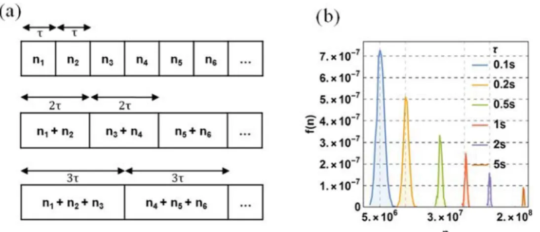
Figure 1.(a) Schematic representation of the simple algorithm used for obtaining photon counts at diﬀerent integration times from a single trace sampled withτ time. When τ ≫ Tc, any niand njare uncorrelated and independent of one another. Using this algorithm, the sample size decreases

systematically as the integration time increases. (b) The probability density distribution of photon counts constructed at six integration times (log− lin scale). f(n)× dn quantiﬁes the probability that the photon count number is found in dn interval about n. The depolarized scattering from a dilute aqueous suspension of tCNCs was observed atθ = 150°.

(5)

variables. By having the sampling distribution at hand, the expectable accuracy and precision of Tccan be calculated in the same manner as that forδ and for any sample size. Naturally, the same is true for Tc−1and the hydrodynamic radius.

■

RESULTS

We collected photons using a commercial instrument designed and built for correlation spectroscopy. The low concentration and the nonfocused beam used in our experiments ensured that the speckle fluctuations were independent of one another.24 There was only one available time resolution to count photons. The sampling rate was relatively low, ∼9.5 Hz, which corresponds to an integration time ofτ = 0.105 s. Accordingly, we had to collect photons during relatively long measurements. Photons from tCNCs were collected for t = 300 s and those from SiO2, for t = 600 s. These lengths defined maximum sample sizes of 2857 and 5714, respectively. Photon traces with 2τ, 3τ, 4τ, and so forth were constructed as illustrated inFigure 1a.Figure 1b shows the influence of the integration time on the probability density distribution of photon counts. The mean value is proportional to the integration time, whereas the relative width of the distribution decreases with τ.

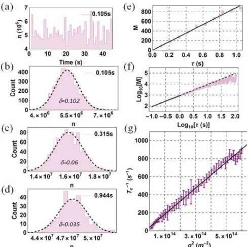
tCNCs. Figure 2a shows a part of a photon trace of depolarized light scattering from a dilute aqueous suspension of tCNCs. Indeed, as is predicted byeqs 1−4, the distributions of photon counts followed normal distributions, and the coeﬃcient of variation δ decreased with integration time (Figure 2b−d).

Following eq 4, the dynamics of Brownian motion can be determined via the dependence ofδ on τ.Figure 2e,f shows that M was linearly proportional to τ. Via eq 2 and a linear regression, we determined a coherence time of Tc= 1.04 ms.

Figure 2f shows M as a functionτ computed over 3 orders of magnitude. We found that the linear relationship was valid over a wide range, and the agreement between theoretical prediction and experimental evidence was preserved up to τ ≈ 20 s (Log10[τ(s)] = 1.3). Above this value, however, some deviation was appreciable. Given that the sample size was systematically decreasing with increasing τ, we attribute this deviation to statistical ﬂuctuations.

To probe the scattering-angle dependence of the observed Brownian dynamics, we collected photon traces at several scattering angles (Figure 2g). The relaxation rate corresponding to translation diﬀusion was found to be proportional to q2_, whereas the relaxation rate of the speckle ﬂuctuations

Figure 2.Analysis of photon counts of depolarized scattering from an aqueous suspension of tCNCs. (a−f) the scattering angle was θ = 150°. (a) Plot showing the numbers of photons counted over 45 s withτ = 0.105 s integration time. (b−d) Distributions of photon counts obtained at three diﬀerent integration times. The dashed lines show unadjusted Gaussian functions corresponding to the mean and the variance of the respective photon counts. The numbers typed in italic are the coeﬃcients of variation of the photon counts (eq 1). (e) Plot of M as a function ofτ (symbol) and the linear regression to the data pairs. (f) Plot of the logarithms of M andτ on an extended range (0.105 s ≤ τ ≤ 100.5 s). The solid line is redrawn from panel (e), and the dashed line is the extrapolation of the solid line. (g) Plot showing the q2_{-dependence of the relaxation rate}

determined from depolarized speckle-visibility analysis (15° ≤ θ ≤ 150°). Each value of M was obtained as shown in panel (e), and Tcwas obtained

usingeq 2. The uncertainty (error bar) is given by the standard deviation determined from 10 measurements per angle. The solid line is a linear regression.

(6)

corresponding to rotational dynamics was expected to be independent of the scattering angle

= +

−

Tc 1 6DR q D2 T (10)

The diffusion coefficients, DRand DT, correspond to rotational (DR) and translational (DT) diffusivity, respectively.

5,25

kBis the Boltzmann constant, T is temperature,η is the viscosity of the solvent, q is the momentum transferq= 4_λπn sin

( )

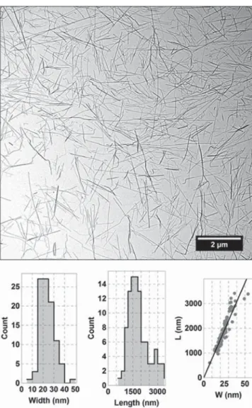
θ₂ ,θ is the scattering angle,λ is the wavelength of the scattered waves, and n is the refractive index of the suspension.Equation 10defines a straight line, and indeed, the results of the statistical analysis of the photon count traces recorded at several scattering angles showed this tendency (Figure 2g). The corresponding line has two independent parameters: a slope and an intercept, which relate to the translational and rotational diffusivities, which in turn are related to the dimensions of the tCNCs. The diffusion coefficients of long and straight rods can generally be expressed by a common form26,27 πη = D k T L W L 3 ln( / ) R B 3 ₍₁₁₎ πη = D k T L W L 3 ln( / ) T B (12)

where L and W are the length and width, and L/W is the aspect ratio. Equations 11 and12 do not take into account whether the ends of the rods areflat or round, which in fact can affect Brownian dynamics when the aspect ratio is small. Given that the tCNCs have a high aspect ratio (Figure 3), this was not a concern in our analysis. The linear regression (Figure 2g, solid line) determined an intercept of (40.13± 4.3) s−1and a slope of (1.45 ± 0.02) × 10−12 m−2 s−1. Via eq 10−12 and by applying the rule of propagation of small independent errors, we obtained an average length (L) of (1394 ± 75) nm and width (W) of (13 ± 3.4) nm. These values are in good agreement with values reported elsewhere,28 and are also consistent with our TEM analysis (Figure 3). The TEM micrograph shows that the tCNCs are dominantly straight and exhibit a high aspect ratio. Via image analysis, we estimated a width of W = 24± 7 nm, a length of L = 1858 ± 620 nm, and an aspect ratio of L/W = 77± 9. The length and width exhibit a clear correlation with a correlation coefficient = 0.92.

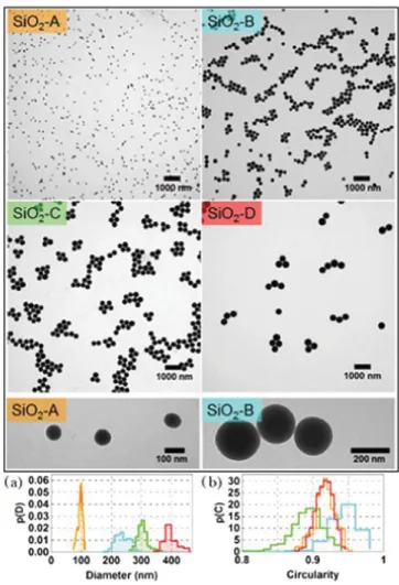
Silica Particles. TEM micrographs of the SiO2particles and the results of the image analyses are shown in Figure 4. The orientation-averaged Feret diameters exhibit small dispersions, and the coeﬃcients of variation are below 10% (Figure 4a). The mean diameters determined by image analysis are 96, 238, 305, and 397 nm for SiO2-A, SiO2-B, SiO2-C, and SiO2-D, respectively. As shown by two close-up views, the existence of shape anisotropyresulting from slight elongation and moderate deformationsis evident. We quantiﬁed the degree of shape anisotropy by the circularity (Figure 4b), which measures the deviation of the perimeter of the particle from a perfect sphere with a smooth surface. The circularity was found to be below onethe mean values are 0.92, 0.94, 0.89, and 0.92 for SiO2-A, SiO2-B, SiO2-C, and SiO2-D, respectively indicating anisotropic polarizability and leading to a small but nonvanishing depolarization ratio.6,29

The depolarization ratio of the silica particles is much smaller than that of the tCNCs, and due to their low concentration and relatively large diameter, the intensity of depolarized scattering

in our instrument was only sufficiently high at lower scattering angles. Therefore, we did not access the whole full q-range, and restricted our analysis to one angle (θ = 30°).Figure 5shows the SVS analysis of depolarized light scattered from dilute suspensions of silica particles. The analyses were performed as in the case of tCNCs but this time the intensity autocorrelation function g2 was also computed for PCS analysis. The field autocorrelation function g1 was obtained from the intensity autocorrelation function, via the Siegert relationg₁= g₂−1. To determine the relaxation rate via PCS, the experimental spectra were fitted against a single negative exponential function: g1(t) = e−t/Tc(Figure 5c).

Table 1lists the correlation times of theﬂuctuations of the depolarized speckles obtained via SVS and PCS. For comparison, the TEM results are also included. The agreement between the two techniques is indeed very good. The sphere-equivalent hydrodynamic radii were estimated viaeq 10, where

πη = D k T r 8 1 R B 3 (13) and

Figure 3.Top: TEM micrograph of the tCNCs used. Bottom: Width

and length distribution functions of the tCNCs obtained from TEM image analysis.

(7)

πη = D k T r 6 1 T B (14)

correspond to the rotational (DR) and translational (DT) diﬀusivities of a perfect sphere of radius r, respectively.5,25,30−32

In comparison to the dimensions established by TEM, both SVS and PCS supplied larger particle sizes, except for SiO2-D, where the average diameter determined by TEM is slightly larger (6 and 4%, respectively).

■

DISCUSSION

We have demonstrated the equivalence of SVS and PCS in determining the coherence times of speckle fluctuations resulting from depolarized light scattering. Our approach has a few potential benefits. First, the theory shows that the statistics of relatively small samples are highly accurate if one has the possibility to collect a sufficiently large number of independent samples. We point out that to not affect the correlation coefficients, PCS requires that the photon trace is fully continuous along its length (t ≫ Tc), and that the integration time is much smaller than the relaxation time (τ ≪ Tc). Our approach, on the other hand, is not limited by these requirements and therefore offers more flexibility. In particular,

when using one single detector, it enables time-shared multiplexing either between different optical lines aligned to observe different q-values and/or between polarized versus depolarized modes (standard DLS vs DDLS), whose combination enables better characterization.33This also waives the necessity of a motorized precision goniometer and the utilization of multiple parallel detection/correlation units, which are required for multiangle DLS apparatus (MALS or MDLS).14,34 A lower price−performance ratio is evidently desirable when anticipating an eventual priority of miniatur-ization and integration of depolarized light scattering into, for example, microfluidic lab-on-a-chip platforms dedicated to automation and parallelization for high-throughput.35−41

Moreover, the coherence time can be accurately measured no matter how small Tc is, as long as Cr · Tc ≫ 1; Cr is the counting rate defined as the average number of photons detected per second Cr = ⟨n(τ)⟩τ−1. The usual unit of the counting rate is Hz, that is, Cr = 100 kHz means that on average 105_{photons are counted in a second. Therefore, a low} temporal resolutioneven several orders of magnitude smaller than the relaxation rate of the depolarized speckle fluctuation itselfcan be sufficiently sensitive for determining Brownian dynamics if one works with high-average photon count rates. This is in striking contrast to photon correlation analysis, which requires a temporal resolution that is several orders of magnitude smaller than the correlation time. This implies that when PCS fails to provide the sufficient temporal resolution and dynamic range, photon counting may solve the problem by replacing the necessity of a high temporal resolution with that of a high counting rate.

In addition, speckle fluctuations represent a stationary and ergodic stochastic process. This, in essence, means that the statistical moments are time invariant and can be estimated from a single but sufficiently large sample of the process, and that time averages and ensemble averages are equivalent. There are noteworthy benefits of exploiting stationarity and ergodicity. Instead of analyzing time averages, one may analyze ensemble averages. For example, by imaging the speckle pattern onto the pixels of a camera, a single“static” snapshot recorded with τ exposure (as integration time) will, in fact, carry the same information about Brownian dynamics as the temporal photon counts do. Therefore, information describing structure (static light scattering,⟨n(τ)⟩) and Brownian dynamics can be obtained simultaneously at once. Consequently, the statistical analysis on a multitude of single speckles is equivalent to that obtained via one single detector, or equivalently, by one single pixel. Furthermore, a two-dimensional area detector intrinsi-cally provides q-space resolved access to Brownian dynamics. Simultaneous access to multiple q-values within a single snapshot ofτ exposure is an option that may have considerable advantages, including rapidity and dense information content.

Finally, photon counting oﬀers a means to handle a large intensity burst caused by“foreign” scattering centers (typically dust and aggregates). The presence of outliers and intensity drift deteriorates the correlation function, and hence, corrupts PCS analysis. The negative impact of this can be mitigated only when certain conditions are satisﬁed.42Although outliers and drift can be easily recognized in a photon stream and rejected once the photon count distribution is constructed,24their real-time exclusion from a photon stream has pitfalls.43

Figure 4. TEM analysis of the SiO2 particles used. In top frame:

micrographs and close-up views of SiO2 particles. Bottom: (a) The

distributions of the orientation-averaged Feret diameters. Orange: SiO2-A (mean 96 nm), cyan: SiO2-B (238 nm), green: SiO2-C (305

nm), and red: SiO2-D (397 nm). (b) The distributions of the

circularities (orange: SiO2-A, cyan: SiO2-B, green: SiO2-C, and red:

SiO2-D).

(8)

■

SUMMARY

We presented an experimental approach to study Brownian dynamics through the statistical analysis of depolarized speckles. By identifying a simple linear scalingwhich is valid over a broad dynamic rangewe established a straightforward relationship between photon count statistics and Brownian dynamics. We treated as well as tested exhaustively the expectable accuracy and precision. Theory and experiments were found to be in very good agreement. To the best of our knowledge, this approachbeing analogous to SVS4 and a viable alternative to diﬀerential dynamic microscopy44is new to depolarized DLS and can provide beneﬁts. Finally, the theory is also valid for standard polarized scattering if the corresponding relationships are used.

■

ASSOCIATED CONTENT

*

S Supporting Information

The Supporting Information is available free of charge on the

ACS Publications website at DOI:10.1021/acs.jpcb.7b04971. Additional analyses and experimental evidence (PDF)

■

AUTHOR INFORMATION Corresponding Author *E-mail:[email protected]. ORCID Christoph Weder: 0000-0001-7183-1790 Alke Petri-Fink: 0000-0003-3952-7849 Sandor Balog: 0000-0002-4847-9845 Author Contributions

S.B. conceived the project, developed the analytical approach, derived the theoretical treatment, and carried out and analyzed the depolarized light scattering experiments. J.N. isolated the tCNCs and performed their TEM analysis. D.B. and D.A.U. synthesized the SiO2 particles. D.B. collected and edited the TEM micrographs. S.B. wrote the manuscript with contribu-tions of all co-authors. All co-authors have given approval to the ﬁnal version of the manuscript and none of the authors declares any competingﬁnancial interest.

Notes

The authors declare no competing ﬁnancial interest.

■

ACKNOWLEDGMENTS

The authors are grateful for the ﬁnancial support of the Adolphe Merkle Foundation and the University of Fribourg. We acknowledge the ﬁnancial support of the Swiss National Science Foundation through the National Center of Com-petence in Research Bio-Inspired Materials, the National Research Program “Resource Wood” (136976 and 136911), and Grant# PP00P2126483/1 (A.P.-F.).

■

REFERENCES

(1) Merkus, H. G.; Meesters, G. M. H. Particulate Products: Tailoring Properties for Optimal Performance; Springer International Publishing, 2014.

(2) Borsali, R.; Pecora, R. Soft Matter Characterization; Springer: Netherlands, 2008.

Figure 5.Speckle-visibility spectroscopy (SVS) and PCS analyses of depolarized scattering from the SiO2-A−D particles (θ = 30°). (a) Plots of M as

a function ofτ (symbol), and linear regressions (solid lines). (b) Plots of the logarithm of M and τ on an extended scale (0.105 s ≤ τ ≤ 100.5 s). The solid lines are redrawn from panel (a), and the dashed lines are extrapolations of the solid lines. (c) Theﬁeld autocorrelation functions obtained via PCS and the correspondingﬁts according to a negative exponential function.

Table 1. Coherence Times and Hydrodynamic Diameters Obtained by SVS and PCSa

coherence time Tc(μs) diameter (nm) SVS PCS SVS PCS TEM SiO2-A 372± 2 428± 15 146± 1 153± 2 96 SiO2-B 1809± 19 1706± 72 255± 1 250± 4 238 SiO2-C 3520± 27 3502± 183 327± 1 326± 7 305 SiO₂-D 5322± 35 5658± 178 373± 1 382± 5 397 a_{Depolarized scattering from SiO}

2-A−D particles was observed at θ =

30°. The errors indicated represent standard errors of the parameter ﬁts (SVS, PCS).

(9)

(3) Goodman, J. W. Statistical Optics; Wiley, 2000.

(4) Bandyopadhyay, R.; Gittings, A. S.; Suh, S. S.; Dixon, P. K.; Durian, D. J. Speckle-Visibility Spectroscopy: A Tool to Study Time-Varying Dynamics. Rev. Sci. Instrum. 2005, 76, No. 093110.

(5) Pecora, R. Dynamic Light Scattering: Applications of Photon Correlation Spectroscopy; Plenum Press: New York, 1985.

(6) Geers, C.; Rodriguez-Lorenzo, L.; Andreas Urban, D.; Kinnear, C.; Petri-Fink, A.; Balog, S. A New Angle on Dynamic Depolarized Light Scattering: Number-Averaged Size Distribution of Nanoparticles in Focus. Nanoscale 2016, 8, 15813−15821.

(7) Levin, A. D.; Shmytkova, E. A.; Khlebtsov, B. N. Multi-polarization Dynamic Light Scattering of Nonspherical Nanoparticles in Solution. J. Phys. Chem. C 2017, 121, 3070−3077.

(8) Levin, A. D.; Lobach, A. S.; Shmytkova, E. A. Study of Geometric Parameters of Nonspherical Nanoparticles by Partially Depolarized Dynamic Light Scattering. Nanotechnol. Russ. 2015, 10, 400−407.

(9) Levin, A. D.; Shmytkova, E. A.; Min’kov, K. N. Determination of the Geometric Parameters of Gold Nanorods by Partially Depolarized Dynamic Light Scattering and Absorption Spectrophotometry. Meas. Tech. 2016, 59, 709−714.

(10) Brown, R. G. W.; Smart, A. E. Practical Considerations in Photon Correlation Experiments. Appl. Opt. 1997, 36, 7480−7492.

(11) Kojro, Z.; Riede, A.; Schubert, M.; Grill, W. Systematic and Statistical Errors in Correlation Estimators Obtained from Various Digital Correlators. Rev. Sci. Instrum. 1999, 70, 4487−4496.

(12) Kojro, Z. Influence of Statistical Errors on Size Distributions Obtained from Dynamic Light Scattering Data: Simulation of Experimental Noise in the Intensity Autocorrelation Function. J. Mod. Opt. 1991, 38, 1867−1878.

(13) Schätzel, K. Correlation Techniques in Dynamic Light

Scattering. Appl. Phys. B 1987, 42, 193−213.

(14) Bantchev, G. B.; Russo, P. S.; McCarley, R. L.; Hammer, R. P. Simple Multiangle, Multicorrelator Depolarized Dynamic Light Scattering Apparatus. Rev. Sci. Instrum. 2006, 77, No. 043902.

(15) Capadona, J. R.; Van Den Berg, O.; Capadona, L. A.; Schroeter, M.; Rowan, S. J.; Tyler, D. J.; Weder, C. A Versatile Approach for the Processing of Polymer Nanocomposites with Self-Assembled Nano-fibre Templates. Nat. Nanotechnol. 2007, 2, 765−769.

(16) Giesche, H. Synthesis of Monodispersed Silica Powders I. Particle Properties and Reaction Kinetics. J. Eur. Ceram. Soc. 1994, 14, 189−204.

(17) Urban, C.; Schurtenberger, P. Characterization of Turbid Colloidal Suspensions Using Light Scattering Techniques Combined with Cross-Correlation Methods. J. Colloid Interface Sci. 1998, 207, 150−158.

(18) Ridler, T. W.; Calvard, S. Picture Thresholding Using an Iterative Selection Method. IEEE Trans. Syst., Man, Cybern. 1978, 8, 630−632.

(19) Mandel, L.; Sudarshan, E. C. G.; Wolf, E. Theory of Photoelectric Detection of Light Fluctuations. Proc. Phys. Soc. 1964, 84, 435.

(20) Jakeman, E.; Pike, E. R. The Intensity-Fluctuation Distribution of Gaussian Light. J. Phys. A: Gen. Phys. 1968, 1, 128.

(21) McKay, A. T. Distribution of the Coefficient of Variation and the Extended“T” Distribution. J. R. Stat. Soc. 1932, 95, 695−698.

(22) Forkman, J.; Verrill, S. The Distribution of Mckay’s Approximation for the Coefficient of Variation. Stat. Probab. Lett. 2008, 78, 10−14.

(23) Peyton, Z.; Peebles, J. Probability, Random Variables, and Random Signal Principles; New York: McGraw-Hill, 1987.

(24) Balog, S.; Zakharov, P.; Scheffold, F.; Skipetrov, S. E. Photocount Statistics in Mesoscopic Optics. Phys. Rev. Lett. 2006, 97, No. 103901.

(25) Debye, P. Polar Molecules; Dover: New York, 1929.

(26) Ortega, A.; Torre, J. G. d. l. Hydrodynamic Properties of Rodlike and Disklike Particles in Dilute Solution.J. Chem. Phys. 2003, 119, 9914−9919.

(27) Kirkwood, J. G. The General Theory of Irreversible Processes in Solutions of Macromolecules. J. Polym. Sci. 1954, 12, 1−14.

(28) Zhao, Y.; Zhang, Y.; Lindström, M. E.; Li, J. Tunicate Cellulose Nanocrystals: Preparation, Neat Films and Nanocomposite Films with Glucomannans. Carbohydr. Polym. 2015, 117, 286−296.

(29) Khlebtsov, N. G.; Melnikov, A. G.; Bogatyrev, V. A.; Dykman, L. A.; Alekseeva, A. V.; Trachuk, L. A.; Khlebtsov, B. N. Can the Light Scattering Depolarization Ratio of Small Particles Be Greater Than 1/ 3? J. Phys. Chem. B 2005, 109, 13578−13584.

(30) Einstein, A. The Motion of Elements Suspended in Static Liquids as Claimed in the Molecular Kinetic Theory of Heat. Ann. Phys. 1905, 332, 549−560.

(31) Einstein, A. Eine Neue Bestimmung Der Moleküldimensionen. Ann. Phys. 1906, 324, 289−306.

(32) Einstein, A. Berichtigung Zu Meiner Arbeit: “Eine Neue

Bestimmung Der Moleküldimensionen”. Ann. Phys. 1911, 339, 591− 592.

(33) Balog, S.; Rodriguez-Lorenzo, L.; Monnier, C. A.; Michen, B.; Obiols-Rabasa, M.; Casal-Dujat, L.; Rothen-Rutishauser, B.; Petri-Fink, A.; Schurtenberger, P. Dynamic Depolarized Light Scattering of Small Round Plasmonic Nanoparticles: When Imperfection Is Only Perfect. J. Phys. Chem. C 2014, 118, 17968−17974.

(34) Shetty, A. M.; Wilkins, G. M. H.; Nanda, J.; Solomon, M. J. Multiangle Depolarized Dynamic Light Scattering of Short Function-alized Single-Walled Carbon Nanotubes. J. Phys. Chem. C 2009, 113, 7129−7133.

(35) Sorensen, C. M. Light Scattering as a Probe of Nanoparticle Aerosols. Part. Sci. Technol. 2010, 28, 442−457.

(36) Rogers, R. B.; Meyer, W. V.; Zhu, J.; Chaikin, P. M.; Russel, W. B.; Li, M.; Turner, W. B. Compact Laser Light-Scattering Instrument for Microgravity Research. Appl. Opt. 1997, 36, 7493−7500.

(37) Chastek, T. Q.; Beers, K. L.; Amis, E. J. Miniaturized Dynamic Light Scattering Instrumentation for Use in Microfluidic Applications. Rev. Sci. Instrum. 2007, 78, No. 072201.

(38) Destremaut, F.; Salmon, J.-B.; Qi, L.; Chapel, J.-P. Microfluidics with on-Line Dynamic Light Scattering for Size Measurements. Lab Chip 2009, 9, 3289−3296.

(39) Chastek, T. Q.; Iida, K.; Amis, E. J.; Fasolka, M. J.; Beers, K. L. A Microfluidic Platform for Integrated Synthesis and Dynamic Light Scattering Measurement of Block Copolymer Micelles. Lab Chip 2008, 8, 950−957.

(40) Denis, P.; Thomas, Q. C. A Versatile, Low-Cost Approach to Dynamic Light Scattering. Meas. Sci. Technol. 2009, 20, No. 045705.

(41) Chen, Z.; Hu, P.; Meng, Q.; Dong, X. Novel Optical Fiber Dynamic Light Scattering Measurement System for Nanometer Particle Size. Adv. Mater. Sci. Eng. 2013, 2013, 1.

(42) Dynamics of Macromolecular Motion. In Photon Correlation Spectroscopy and Velocimetry; Cummins, H. Z., Pike, E. R., Eds.; Springer, 1977.

(43) Haller, H. R.; Destor, C.; Cannell, D. S. Photometer for Quasielastic and Classical Light Scattering. Rev. Sci. Instrum. 1983, 54, 973−983.

(44) Fabio, G.; Catalina, H.-P.; Roberto, C. Simultaneous Character-ization of Rotational and Translational Diffusion of Optically Anisotropic Particles by Optical Microscopy. J. Phys.: Condens. Matter 2016, 28, No. 195201.