Evidence on a link between the intensity of Schumann resonance and global surface temperature

HAL Id: hal-00318115

https://hal.archives-ouvertes.fr/hal-00318115

Submitted on 9 Aug 2006

HAL is a multi-disciplinary open access

archive for the deposit and dissemination of

sci-entific research documents, whether they are

pub-lished or not. The documents may come from

teaching and research institutions in France or

abroad, or from public or private research centers.

L’archive ouverte pluridisciplinaire HAL, est

destinée au dépôt et à la diffusion de documents

scientifiques de niveau recherche, publiés ou non,

émanant des établissements d’enseignement et de

recherche français ou étrangers, des laboratoires

publics ou privés.

Evidence on a link between the intensity of Schumann

resonance and global surface temperature

M. Sekiguchi, M. Hayakawa, A. P. Nickolaenko, Y. Hobara

To cite this version:

M. Sekiguchi, M. Hayakawa, A. P. Nickolaenko, Y. Hobara. Evidence on a link between the intensity

of Schumann resonance and global surface temperature. Annales Geophysicae, European Geosciences

Union, 2006, 24 (7), pp.1809-1817. �hal-00318115�

© European Geosciences Union 2006

Geophysicae

Evidence on a link between the intensity of Schumann resonance

and global surface temperature

M. Sekiguchi1, M. Hayakawa1, A. P. Nickolaenko2, and Y. Hobara1,3

1_{The University of Electro-Communications, Department of Electronic Engineering, Chofu, Tokyo, Japan}

2_{Usikov’s Institute for Radiophysics and Electronics, National Academy of Science of the Ukraine, Kharkov, Ukraine} 3_{Swedish Institute of Space Physics, Kiruna, Sweden}

Received: 19 August 2005 – Revised: 12 June 2006 – Accepted: 14 June 2006 – Published: 9 August 2006

Abstract. A correlation is investigated between the intensity of the global electromagnetic oscillations (Schumann reso-nance) with the planetary surface temperature. The electro-magnetic signal was monitored at Moshiri (Japan), and tem-perature data were taken from surface meteorological obser-vations. The series covers the period from November 1998 to May 2002. The Schumann resonance intensity is found to vary coherently with the global ground temperature in the latitude interval from 45◦S to 45◦N: the relevant cross– correlation coefficient reaches the value of 0.9. It slightly in-creases when the high-latitude temperature is incorporated. Correspondence among the data decreases when we reduce the latitude interval, which indicates the important role of the middle-latitude lightning in the Schumann resonance oscilla-tions. We apply the principal component (or singular spec-tral) analysis to the electromagnetic and temperature records to extract annual, semiannual, and interannual variations. The principal component analysis (PCA) clarifies the links between electromagnetic records and meteorological data. Keywords. Meteorology and atmospheric dynamics (Atmo-spheric electricity; Climatology) – Radio science (Remote sensing)

1 Introduction

A correspondence was demonstrated by Williams (1992) be-tween the long-term Schumann resonance amplitude and the temperature anomaly in the tropical belt. The global electro-magnetic or Schumann resonance is a phenomenon that takes place in the spherical Earth-ionosphere cavity (Nickolaenko and Hayakawa, 2002). Oscillations are maintained by the global lightning activity, which radiates the extremely low frequencies (ELF). The intensity of the resonance reflects

Correspondence to: M. Hayakawa

(hayakawa@whistler.ee.uec.ac.jp)

the instantaneous level of thunderstorm activity, and it must vary with the global temperature. Williams (1992) used the Schumann resonance records collected by Charles Polk at the Rhode Island field site; the duration covered six years (Polk, 1969, 1982). We show in Fig. 1 the plot adopted from Williams (1992), where the electromagnetic data are com-pared with the monthly mean fluctuation in the surface (dry-bulb) temperature for the entire tropics. Time is shown on the abscissa, the global temperature anomaly in the tropical region is shown along the right ordinate in centigrade (the heavy line), and the amplitude is plotted on the left ordinate measured in the horizontal magnetic field at the fundamental mode of Schumann resonance (the line with open squares). As one may see, Fig. 1 shows that the Schumann resonance amplitude follows the temperature anomaly quite closely for the long-period variation.

An interest in the Schumann resonance reappeared in the 90s. Many observatories were set at work (Sentman, 1995; Satori and Zieger, 1996; F¨ullekrug and Fraser-Smith, 1997; Nickolaenko, 1997; Nickolaenko et al., 1998, 1999; Heck-man et al., 1998; Hobara et al., 2000, 2001, 2003; Hayakawa et al., 2004), and noticeable progress was made in the Schu-mann resonance modeling (Kirillov et al., 1997; Hayakawa and Otsuyama, 2002; Mushtak and Williams, 2002; Ot-suyama et al., 2003; Simpson and Taflove, 2004; Yang and Pasko, 2005). The present work is a further development of the idea by Williams (1992), Price (1993), F¨ullekrug and Fraser-Smith (1997), and Williams (1994). We inves-tigate the relationship between the Schumann resonance in-tensity and the global soil temperature, the latter was mea-sured in symmetric latitudinal intervals. The driving idea is rather straightforward. Electromagnetic radiation from the global lightning strokes is the source of electromagnetic en-ergy detected in the Schumann resonance band (from a few Hz to some tens of Hz). The planetary thunderstorm activ-ity is concentrated in the tropics. The lightning flash rate is collected from space, using the optical transient detector

1810 M. Sekiguchi et al.: Schumann resonance and global surface temperature

1

Fig.1 Correlation between the global temperature and the intensity of Schumann resonance oscillations (adopted from Williams (1992)).

Fig. 1. Correlation between the global temperature and the intensity of Schumann resonance oscillations (adopted from Williams, 1992).

(OTD) (Orville and Henderson, 1986; Christian et al., 2003; Hayakawa et al., 2005). The lightning flash is high in the tropics, remains relatively high in the mid-latitudes, and be-comes rare in the polar and sub-polar regions. Therefore, one may expect that the Schumann resonance intensity is con-nected with the surface temperature within a certain latitudi-nal interval. We are going to test this idea and establish the width of such an interval.

By following the Sun, global thunderstorms cyclically drift along the meridian to the Northern Hemisphere dur-ing boreal summer, and drift southward from the equator in winter. Since the continents occupy a greater area in the Northern Hemisphere, an annual variation develops in the thunderstorm activity: the global flash rate is smaller dur-ing the winter months (Christian et al., 2003; Hayakawa et al., 2005). Therefore, annual variations must also be present in the Schumann resonance intensity. The goal of our in-vestigation is a formal comparison of trends present in the Schumann resonance intensity and the ground temperature itself.

We correlate the long-term seasonal variations of cumula-tive intensity of three Schumann resonance modes with the changes in the median global land temperature relevant to different symmetric latitudinal belts. We look for the inter-val where the close correlation appears between the climato-logical and electromagnetic data. Afterwards, to remove the random oscillations always present in the data sets, we turn to the principal components (Troyan and Hayakawa, 2003), namely, to the annual, semiannual and interannual trends, which are extracted from the raw temperature and Schumann resonance data. Finally, the current results are discussed and

explained, and the areas of future work are outlined.

2 Acquisition of Schumann resonance data and signal

processing

The natural ELF signal is monitored at the Moshiri obser-vatory (Japan, 44◦220N and 142◦150E) since 1996. Two orthogonal horizontal magnetic field components (HN S and

HEW) and one vertical electric field component (EZ) are

recorded simultaneously; the details are found in Hobara et al. (2001). In this paper, we discuss the continuous time se-ries of the horizontal HN Sfield component, covering the

pe-riod from November 1998 to May 2002. The longest contin-uous data set is available in this particular component (with a few data gaps). The other components, unfortunately, have greater gaps caused by the local interferences or by the tem-poral system malfunction. In addition, the EZrecords suffer

from the bad weather conditions.

The notation of HN Scorresponds to the magnetic coil

an-tenna aligned to the local meridian; such a sensor is sensitive to the radio waves arriving from the east (thunderstorms in America) or from the west (African activity). The ELF mea-surement system is periodically calibrated.

The power spectra of the Schumann resonance are com-puted during the processing of a record with the FFT al-gorithm. Spectra are averaged over segments 10 min long. These data are additionally averaged over each hour of the day, which allows us to reduce the impact of data gaps on the output results. Finally, the monthly mean is computed for every hour. Thus, we obtain the monthly averaged spectra as the function of universal time. These sets were ultimately

M. Sekiguchi et al.: Schumann resonance and global surface temperature 1811 '99.1 7 '00.1 7 '01.1 7 '02.1 0 6 12 18 24 Month, Year Ti m e [U T] 0.2 0.4 0.6 0.8 1.0 1.2 -6 -5 -4 -3 -2 -1 0 [dB] [pT2_]

Fig.2 Monthly averaged diurnal variation of the cumulative energy of Schumann resonance. The color code is used to indicate the absolute intensity (in pT2_{) (and also in dB).}

Fig. 2. Monthly averaged diurnal variation of the cumulative

en-ergy of Schumann resonance. The color code is used to indicate the absolute intensity (in pT2)(and also in dB).

averaged to produce the median Schumann resonance spectra relevant to each month of a year.

Schumann resonance is observed as the peaks (modes) in the power spectrum of the given field component. Each mode corresponds to a particular spatial distribution of the field. Thunderstorms move around the globe during the day, the distance from an observatory to the lightning sources varies, and the amplitude of individual Schumann resonance modes also varies. Alterations caused by the source position are superimposed on the changes connected with the contempo-rary intensity of the global thunderstorm activity. So, when obtaining the estimates of thunderstorm intensity, we have to reduce the impact of distance variations. The cumulative in-tensity of three Schumann resonance modes is used for this purpose, being less sensitive to the source–observer distance (see Polk, 1969, Sentman and Fraser, 1991; Nickolaenko, 1997, Nickolaenko et al., 1999, Nickolaenko and Hayakawa, 2002):

I = A2₁+A2₂+A2₃. (1)

Here, Ai is the magnetic field amplitude of the i-th mode

(i=1, 2, 3). We use the ±0.5-Hz bandwidth for each mode. This approach was exploited in the experimental studies of

'99.1 7 '00.1 7 '01.1 7 '02.1 7 0.2 0.3 0.4 0.5 0.6 0.7 0.8 0.9 1 S R In te n s it y [p T 2] '99.1 7 '00.1 7 '01.1 7 '02.1 7 -6 -5 -4 -3 -2 -1 0 S R In te n s it y [d B ] '99.1 7 '00.1 7 '01.1 7 '02.1 7 10 15 20 25 30 te m per at ur e [ d egr ee]

interval of latitude; +: +/-20, triangle: +/-40, o: +/-60, x: +/-80

Fig.3. Seasonal variations of electromagnetic and temperature data. Top and middle panels show the Schumann resonance intensity in pT2

and in dB correspondingly. Bottom panel presents the global mean ground temperature in symmetric latitudinal belts ±20D, ±40D, ±60D, ±80D.

Fig. 3. Seasonal variations of electromagnetic and temperature data. Top and middle panels show the Schumann resonance in-tensity in pT2and in dB, correspondingly. Bottom panel presents the global mean ground temperature in symmetric latitudinal belts

±20◦, ±40◦, ±60◦, ±80◦.

Schumann resonance when obtaining estimates for the in-stant level of global thunderstorm activity (Clayton and Polk, 1997; Heckman et al., 1998; Nickolaenko et al., 1998, 1999). Figure 2 illustrates the dynamics of the monthly averaged daily variation of the Schumann resonance intensity (1) dur-ing the whole period of observations. The abscissa indicates the month and year, while the ordinate indicates the universal time (UT). The measuring equipment is fully calibrated (Ho-bara et al., 2000), and the presentation in Fig. 2 is given in the absolute intensity (pT2)and in the dB relative to 1 pT2: I[dB]=10 lg(I /IR), where IR=1 pT2. The absolute intensity

observed is in accord with the published data (see Sentman (1995)). The strong American thunderstorm activity is ob-served in the plots of Fig. 2 around midnight (23:00–00:00 hr) UT. A smaller African activity is visible at 14:00–15:00 UT, being somewhat reduced by the angular pattern of the magnetic antenna. An impact of the nearby powerful storms in Southeast Asia is present at 7:00–10:00 UT, even in the HN Sfield component.

1812 M. Sekiguchi et al.: Schumann resonance and global surface temperature

4

Fig.4. Cross-correlation coefficient as the function of latitude interval, for the intensity measured in absolute values (line connected by crosses) and for the intensity measured in dB (line connected by circles). The error bar is also indicated (as the level of confidence of 0.95).

Fig. 4. Cross-correlation coefficient as a function of the latitude

in-terval, for the intensity measured in absolute values (line connected by crosses) and for the intensity measured in dB (line connected by circles). The error bar is also indicated (as the level of confidence of 0.95).

The initial data sets are presented in Fig. 3. The upper panel in Fig. 3 depicts the absolute power (in pT2) of the three Schumann resonance modes (1) as a function of time recorded at Moshiri station from November 1998 to May 2002. The second frame repeats the same plot translated to dB relative to the 1 pT2 scale. The bottom panel presents seasonal variations of the global land surface temperature in different latitudinal intervals. Here the time (in months) is plotted on the abscissa. Vertical dotted lines mark the half– year intervals. As one may see from Fig. 3, the annual vari-ation of the Schumann resonance intensity is close to 5 dB (amplitude variation by a factor of two).

3 Surface temperature data

The bottom panel of Fig. 3 depicts seasonal variations of the surface temperature computed within intervals ranging from 20◦S to 20◦N; 40◦S–40◦N; 60◦S–60◦N; and 80◦S–80◦N. The data were selected from the National Climate Data Cen-ter (USA), which provides monthly mean temperatures for the land area based on the surface meteorological observa-tions (see Petersen and Vose, 1997). Initial data correspond to the grid 15◦×5◦ (longitude times latitude, respectively) covering the entire Earth. The grid mean temperature was calculated for each interval: mean temperature at given lati-tudes was obtained by averaging the grid data in accordance with the ground area found in the interval.

To reduce the impact of seasonal north–south drift, we av-eraged the temperature data in the symmetric latitude inter-vals centered at the equator. Thus, we consistently include the surface temperature of the most important tropical belt, corresponding to the narrow central peak in the latitudinal distribution of lightning flashes observed from space

(Chris-5 24 25 26 27 -6 -5 -4 -3 -2 -1 0 +/- 20 degree T[oC] S R I n tens it y [dB ] 18 19 20 21 22 23 -6 -5 -4 -3 -2 -1 0 +/- 40 degree T[oC] SR In te si ty[d B] 12 13 14 15 16 17 18 19 20 -6 -5 -4 -3 -2 -1 0 +/- 60 degree T[oC] SR In te n s it y[d B ] 11 12 13 14 15 16 17 18 19 -6 -5 -4 -3 -2 -1 0 +/- 80 degree T[oC] SR In te n s it y[d B ]

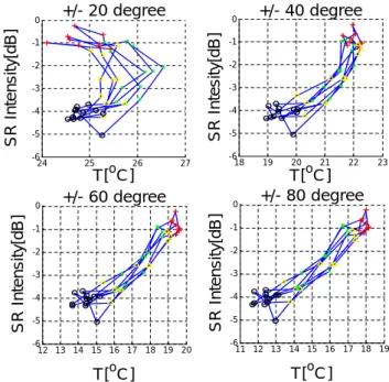
Fig.5. Lissajous figures of the Schumann resonance intensity versus global temperature. Green markers denote the spring, red is the summer, yellow is autumn, and black shows the winter.

Fig. 5. Lissajous figures of the Schumann resonance intensity

ver-sus global temperature. Green markers denote spring, red is sum-mer, yellow is autumn, and black shows winter.

tian et al., 2003; Hayakawa et al., 2005). As might be con-cluded from Fig. 3, this zone is associated with the strong semiannual variation. The north–south seasonal drift and the asymmetry in the global land distribution appear as the an-nual variation in the surface temperature (see the lower plots in Fig. 3 for wide latitudinal gaps). The semiannual variation is always present; however, it seems to diminish in the annual variation pertinent to the middle latitudes. The median tem-perature decreases when the width of the latitudinal interval increases, reflecting the general decline of the temperature with latitude.

4 Correlation between Schumann resonance intensity

and global temperature

We calculated the cross-correlation coefficients for variations of the Schumann resonance intensity and the global ground temperature averaged in different latitudinal belts; see Fig. 4 (the widths of ±5◦_{, ±10}◦_{, ±15}◦_{, etc., were used). The width}

of latitude interval is shown on the abscissa of Fig. 4 in de-grees, and the cross-correlation coefficient is indicated on the ordinate. It seems that a systematically stronger correlation is apparent between the temperature and the Schumann reso-nance intensity measured in dB (crosses) rather than absolute intensity (circles). This property implies that a link between the global temperature and electromagnetic intensity I is of the following form: I =<|H|2>=I0·exp[ζ (T −T0)], where T is current temperature and T0is its median value for the given

latitudinal belt. It is clear that the field level in dB is a mea-sure of the exponent ζ .

One may see from Fig. 4 that the cross-correlation coef-ficient becomes saturated when the latitude interval exceeds ±45◦. Such a behavior might be expected, since the lightning activity is concentrated in the tropics and sub-tropics. On the other hand, a contribution from the mid-latitude temperature into the Schumann resonance intensity (and hence the role of the mid-latitude lightning activity) is significant. The con-clusion is supported by the upper frames of Fig. 3, showing a strong annual variation in the Schumann resonance inten-sity, while the semiannual component prevails in the tropics and sub-tropics. This is the reason why two processes have insignificant cross–correlation until the latitude interval be-comes sufficiently wide.

The connection between two periodic variables, including their mutual phase shift is distinctly demonstrated by the Lis-sajous plots shown in Fig. 5. Here, the seasonal variations of the global soil temperature are plotted on the abscissa. The ordinate shows the Schumann resonance intensity in dB. We use various colors to show different seasons: green marks the spring, the red marks the summer, yellow is autumn, and black is winter. It is easy to see from Fig. 5 that the Schumann resonance intensity and global ground tempera-ture tend to vary coherently. However, their links are com-plicated by the presence of higher harmonics and the phase shifts.

5 Periodic variations of Schumann resonance intensity

and of the global temperature

The pattern of seasonal variation of the surface tempera-ture depends on the width of the latitude interval. It con-sists of two major components: one is the semiannual varia-tion coupled to the tropics, and the other is the annual com-ponent, corresponding to a wider latitude band. There are both annual and semiannual components present in the long-term variations of Schumann resonance parameters. A strong semi-annual variation was found in the frequency of the first resonance mode observed in the vertical electric field compo-nent EZ, which clearly reflects the seasonal variations of the

area covered by the global lightning activity (Nickolaenko et al., 1998). A semiannual variation was also found in the cumulative field intensity recorded in the late 60s in Japan (Nickolaenko et al., 1999). It is interesting to use a simi-lar process for the modern Schumann resonance records and compare the results with the previous data and with concur-rent variations in the global temperature.

We apply the Principal Component Analysis (PCA), which is also regarded in the literature as singular spectral analysis (SSA), to extract periodic components from the Schumann resonance intensity (dB) and from the net global tempera-ture in different latitudinal belts. The software is called the “Caterpillar” algorithm (Troyan and Hayakawa, 2003). We

extract the unknown regular variations which are hidden in the record, and the PCA algorithm is an appropriate tool for this purpose (Danilov and Zhiglyavsky, 1997; Troyan and Hayakawa, 2003). From the physical point of view, the PCA algorithm is similar to filtering, although its main distinction is that the basic functions are found automatically right from the original data.

The algorithm works in the following way. Consider a fi-nite time series of initial data xk=x(tk)with 1 ≤k≤N . An

in-teger number L< N is chosen, called the “caterpillar” length, and the linear set xk is transformed into a 2-D matrix in the

following way. The first L points of the xk series (we use L=12, corresponding to the annual period) occupy the first line of the matrix. The elements from x2to xL+1are placed in the second line, etc. The process continues until we reach the end of the data. The last line of the matrix contains the elements with indices starting from N −L+1, so that the last Lsamples are, xN −L+1, xN −L+2, . . . , xN.

The eigen-values and eigen-vectors are found for the 2-D matrix in the second step of processing. These parameters depend on the signal structure and they allow us simultane-ously to construct the “internal basis” relevant to the data: the so-called principal components. This stage of the pro-cedure is equivalent to composing the bank of linear filters. Each filter corresponds to a particular principal component. We emphasize that filters are found from the data itself rather than postulated beforehand.

In the third step, we visualize, survey, and select the de-sired principal components (PC) revealed in the previous step. The periodic principal components split into pairs: one of them resembles the “sine” wave, while the other is the “co-sine” wave. We usually take PC #1 and PC#2 to obtain the complete annual variation of the lowest frequency.

The final step implies the signal reconstruction by select-ing and combinselect-ing the desired principal components. This step is similar to extracting a set of harmonics in the conven-tional Fourier transform. We must add that the PCA proce-dure turns into an ordinary Fourier transform when the initial succession xk is a sinusoidal signal of infinite duration. In

this case, the matrix constructs authentic sine and cosine ba-sic functions, and the result coincides with the well-known procedures (Danilov and Zhiglyavsky, 1997).

To obtain both annual and semiannual components of the variations of global temperature and Schumann resonance in-tensity, we apply the PCA procedure with the length L=12 (one year) and concentrate our attention on PC#1 and PC#2 (annual variation) and PC#3 and PC#4 (semiannual term). The annual component is present in both temperature and Schumann resonance intensity. A substantial semiannual variation is found only in the global temperature of the trop-ical belt.

The PCA processing also shows that initial data contain only these two major components, plus insignificant ran-dom fluctuations, and we summarize the results in Table 1. The first column of this table denotes the variable. Column

1814 M. Sekiguchi et al.: Schumann resonance and global surface temperature

Table 1. Annual and semiannual components extracted from the data series by the PCA processing.

Variable Annual components, % Semiannual components, %

SR intensity PC#1=49.5 PC#2=45.6 PC#3=1.2 PC#4=1.1 Temperature in ±20◦interval PC#3=9.5 PC#4=8.2 PC#1=34.6 PC#2=33.7 Temperature in ±40◦interval PC#1=43.5 PC#2=40.6 PC#3=7.0 PC#4=6.7 Temperature in ±60◦interval PC#1=49.0 PC#2=46.1 PC#3=2.1 PC#4=2.0

6

Fig.6. Principal components : annual, semi-annual, annual + semi-annual, and interannual. The upper plots refer to the variations of the Schumann resonance intensity, and the lower plots demonstrate the variations of the global soil temperature in different latitude intervals.

Fig. 6. Principal components: annual, semiannual, annual + semiannual, and interannual. The upper plots refer to the variations of the

Schumann resonance intensity, and the lower plots demonstrate the variations of the global soil temperature in different latitude intervals.

numbers 2 and 3 refer to an annual variation, and columns 4 and 5 correspond to a semiannual component. The numbers indicate the contributions of particular principal components into the energy of initial variation. Table 1 indicates that the semiannual term is very small in the Schumann resonance in-tensity: its contribution is below 3%, while the annual varia-tion is responsible for 95%. The semiannual contribuvaria-tion is considerably smaller than in our previous study (about 20%), based on the old resonance data collected in Japan (Nicko-laenko et al., 1999). In contrast, Table 1 shows that the an-nual pattern in the land temperature is of minor importance within the ±20◦_{latitude gap: its contribution is 17% against}

68% from the semiannual trend.

We depict temporal variations of the major principal com-ponents in Fig. 6. Time in months is shown on the abscissa. The ordinate depicts the resonance intensity in dB (upper plots) and temperature in centigrade (lower plots). By com-paring Figs. 6 and 3, one may observe how the PCA pro-cessing “rectified” the variations. Figure 6 presents the an-nual trends (the left frames), semianan-nual terms (the second column of plots), the composition of annual and semiannual variations (the third plot), and interannual variation (the right frames). As is shown in the lower plots of Fig. 6, the am-plitude of the annual temperature variation increases when a wider latitude interval is analyzed. This is explained by

an increase in the north-south asymmetry of the land area in wider latitude intervals. Variations in the ±40◦ and ±60◦ belts occur in phase, while the temperature pattern of ±20◦ latitudinal belt leads in phase by approximately 3 months. Contribution from the polar latitudes into annual variations of global temperature is insignificant (not shown), as was ex-pected. However, the middle latitudes (from 40 to 60 deg) are responsible for a substantial fraction in annual variation of the global land temperature. Amplitude and phase of the semiannual component remain unchanged when we extend the interval of latitudes, as is seen in the second lower plot of Fig. 6. This means that only the tropical region contributes to this semiannual signal.

Plots of Fig. 6 enable us to observe the important features: 1. Variations of electromagnetic intensity and land tem-perature on the annual scale are similar in the wide latitude belts.

2. The beating mode is observed in the semiannual Schu-mann resonance data, which agrees with the published re-sults.

3. Semiannual temperature variations coincide for all the belts, which means that this term originates from the tropical region.

4. General variations of the Schumann resonance inten-sity occur in the way similar to the temperature observed in

M. Sekiguchi et al.: Schumann resonance and global surface temperature 1815 -1 -0.5 0 0.5 1 -2 -1 0 1 2 T [C] SR In te n s it y [d B] -3 -2 -1 0 1 2

Annual vs Annual+Sem i-Annual Com ponent

T [C] SR In te n s it y [d B] -4 -3 -2 -1 0 1 2 3 T [C] SR In te n s it y [d B] -0.5 0 0.5 -2 -1 0 1 2 T [C] SR Int ensity [dB] -3 -2 -1 0 1 2

annual vs Annual Com ponent

T [C] SR Int ensity [dB] -4 -3 -2 -1 0 1 2 3 T [C] SR Int ensity [dB] 23 24 25 26 27 28 -6 -5 -4 -3 -2 -1 0 T [C] SR Intensity [dB] 18 19 20 21 22 23

Initial Data

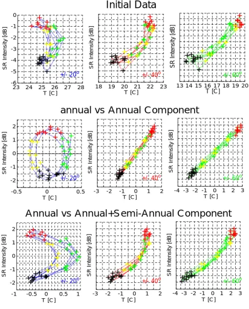
Fig.7. Lissajous figures of global land temperature versus Schumann resonance intensity. The color of plot indicates season (green: spring, red: summer, yellow: autumn, and winter: black).

Table 1 Annual and semi-annual components extracted from the data series by the PCA

Fig. 7. Lissajous figures of global land temperature versus Schumann resonance intensity. The color of plot indicates season (green: spring,

red: summer, yellow: autumn, and winter: black).

the middle latitudes. In contrast, the interannual variations (see the right plots in Fig. 6) exhibit a similarity between the Schumann resonance data and the temperature trends of the topical region. Unfortunately, the 3.5-year duration of the data is somewhat short to extract the interannual alterations with confidence and to make decisive conclusions, however, the similarity must be noted.

We may expect that Lissajous figures will vary when we compare electromagnetic energy with the land temperature of different latitude belts. We show in Fig. 7 the Lissajous patterns of the initial data (the upper line of plots), the an-nual trends (the middle plots), and composition of anan-nual and semiannual components (the lower plots). The Schu-mann resonance intensity is shown on the ordinate of each frame in dB. Variations of temperature are plotted on the ab-scissa. The left column of panels relates the variations of the Schumann resonance intensity with temperature in the

trop-ical ±20◦ region. The central plots correspond to a ±40◦ latitude interval, and the right column depicts the data for a ±60◦belt.

The left frame in the middle row shows that the annual component of temperature in ±20◦ latitudes is in advance by about three months with respect to the annual variations of Schumann resonance intensity. The plot is practically a circle. Annual temperature variations in wider belts occur in phase with the electromagnetic data, and we observe the straight line in the central and right frames of the middle row. The lower plots depict the sums of the annual and semian-nual components extracted from the records. The left plot reminds us of a typical Lissajous figure for two sinusoidal signals, with the frequency ratio 2:1. The central and right plots are just the same in-phase variations of the middle row, but slightly “spoiled” by the “second harmonic”.

1816 M. Sekiguchi et al.: Schumann resonance and global surface temperature

6 Discussion and conclusions

We processed the modern long-term records of the Schu-mann resonance, which have the duration comparable with the former data collected by Prof. K. Sao’s group in the Tottori observatory (Japan) in the 70s (Nickolaenko et al., 1999). The same software was applied toward the new data set. The annual component of the Schumann resonance in-tensity in the modern records is in good correspondence to that found in the old records. The complete annual excur-sion of the Schumann resonance intensity is about 5 dB for the HN S field observed in Japan. Characteristic variation

extracted by the PCA algorithm is somewhat smaller, about ±2 dB. The semiannual component is smaller by an order of magnitude, and this is the main distinction of the new record from the previous data. We cannot indicate the reason of de-viation; however, the data of the 70s contained a strong tem-poral modulation of semiannual pattern, the “beating mode”. It might be that recent records coincide with the period of small amplitude in the semiannual term, owing to some un-known natural factor.

Variations of the Schumann resonance intensity occur in the way similar to the temperature within the middle-latitude interval. In contrast, the interannual variation of Schumann resonance resembles that of temperature in the topics (see the right plots in Fig. 6). Unfortunately, the 3.5-year duration does not allow us to make the decisive conclusions.

A comparison of electromagnetic and temperature data in-dicated that there is a link between the annual variation of the Schumann resonance intensity and the global tempera-ture. The cross-correlation coefficient reaches 0.05, 0.85, 0.92, and 0.95 when we extend the latitude intervals from ±20◦, to ±40◦, ±60◦, and ±80◦, correspondingly.

The data presented in this paper allow us to formulate the following conclusions.

1. Schumann resonance intensity of recent records, 43 months long in duration, made in Japan, is character-ized by a strong annual variation (about ±2 dB), while the semi-annual trend is smaller by an order of magni-tude.

2. Variations in the global land temperature are character-ized by two seasonal patterns associated with different latitude intervals. The semiannual variation dominates in the tropics, and the annual trend prevails in the mid-dle and high latitudes.

3. Intensity variations of Schumann resonance oscillations corresponds to alterations of the global land temperature in the mid-latitude interval of about ±45◦.

Finally, we mention the areas of future works in the Schumann resonance band. Simultaneous observations at a few sites (including those positioned in the Southern Hemi-sphere) are desirable for a reduction of source proximity

ef-fects and separating contributions from thunderstorms in dif-ferent latitude zones. Measurements in the Southern Hemi-sphere are useful, since thunderstorms drift away from the observer in the Southern Hemisphere during boreal sum-mer, and the source distance varies in anti-phase there. The combination of records performed in both hemispheres will compensate for the meridional drift of global thunderstorms, while variations are enhanced associated with the level of global thunderstorm activity itself. Simultaneous observa-tions at a series of staobserva-tions allow for deducing the global dis-tribution of thunderstorm activity (Shvets, 2001; Ando et al., 2005), which can also help to extract alterations in the thun-derstorm activity and thus to improve the quality of initial data.

Acknowledgements. The authors would like to thank M. Sera and

Y. Ikegami of the Moshiri observatory (Nagoya University) for their contribution to the ELF observation there and E. Williams of M. I. T. for his useful comments. Also thanks are due to the unknown refer-ees for their useful comments which helped us to improve the paper. Topical Editor U.-P. Hoppe thanks A. V. Shvets and two other referees for their help in evaluating this paper.

References

Ando, Y., Hayakawa, M., Shvets, A. V., and Nickolaenko, A. P.: Finite difference analyses of Schumann resonance and re-construction of lightning distribution, Radio Sci., 40, no.2, doi:10.1029/2004RS003153, 2005.

Christian, H. J., Blackslee, R. J., Boccippio, D. J., Boek, W. I., Buechler, D. E., Driscoll, K. T., Goodman, S. J., Hall, J. H., Koshak, W. J., Mach, D. M., and Stewart, M. F.: Global fre-quency and distribution of lightning as observed from space by the Optical Transient Detector, J. Geophys. Res., 108 (D1), 4005, doi:10.1029/2002JD002347, 2003.

Clayton, M. and Polk, C. : Diurnal variation and absolute intensity of world-wide lightning activity, September 1970 to May 1971, Electrical Processes in Atmospheres, edited by: Dolezalek, H. and Reiter, R., Steinkopf, Darmstadt Germany, 111–178, 1997. Danilov, D. L. and Zhiglyavsky, A. A. (Eds.): Principal

Compo-nent of the Time Series, the Caterpillar Method (in Russian), St. Petersburg State University, St. Petersburg, Russia, 307, 1997. F¨ullekrug, M. and Fraser-Smith, A. C. : Global lightning and

cli-matic variability inferned from ELF field variations, Geophys. Res. Lett., 24, 2411–2414, 1997.

Hayakawa, M.: Satellite observation of low-latitude VLF radio noise and their association with thunderstorms, J. Geomagn. Geoelectr., 47, 573–595, 1989.

Hayakawa, M. and Otsuyama, T.: FDTD analysis of ELF wave propagation in inhomogencous subionospheric waveguide mod-els, Appl. Computational Electromagnetics Soc. J., 17, No.3, 239–244, 2002.

Hayakawa, M., Nakamura, T., Hobara, Y., and Williams, E. : Ob-servation of sprites over the Sea of Japan and the conditions of lightning-induced sprites in winter, J. Geophys. Res., 109, A01312, doi:10.1029/2003JA009905, 2004.

Hayakawa, M., Sekiguchi, M., and Nickolaenko, A. P.: Diurnal variation of electric activity of global thunderstorms deduced from OTD data, J. Atmos. Electr., 25, 55–68, 2005.

Heckman, S. J., Williams, E., and Boldi, B.: Total global lightning inferred from Schumann resonance measurements, J. Geophys. Res., 103, D24, 31 775–31 779, 1998.

Hobara, Y., Iwasaki, N., Hayashida, T., Tsuchiya, N., Williams, E. R., Sera, M., Ikegami, Y., and Hayakawa, M.: New ELF obser-vation site in Moshiri, Hokkaido, Japan and the results of prelim-inary data analysis, J. Atmos. Electr., 20, 99–109, 2000. Hobara, Y., Iwasaki, N., Hayashida, T., Hayakawa, M., Ohta, K.,

and Fukunishi, H.: Interrelation between ELF transients and ionospheric disturbances in association with sprites and elves, Geophys. Res. Lett., 28, 935–938, 2001.

Hobara, Y., Hayakawa, M., Ohta, K., and Fukunishi, H.: Lightning discharges in association with mesospheric optical phenomena in Japan and their effect on the lower ionosphere, Adv. Polar Upper Atmos. Res., 17, 30–47, 2003.

Kirillov, V. V., Kopeykin, V. N., and Mushtak, V. C.: Electromag-netic waves of ELF band in the Earth–ionosphere waveguide (in Russian), Geomag. Aeron., 37, 114–120, 1997.

Mushtak, V. C. and Williams, E. R.: ELF propagation parameters for uniform models of the Earth–ionosphere waveguide, J. At-mos. Solar-Terr. Phys., 64, 1989–2001, 2002.

Nickolaenko, A. P.: Modern aspects of the Schumann resonance studies, J. Atmos. Solar-Terr. Phys., 59(7), 805–816, 1997. Nickolaenko, A. P., S`atori, G., Ziegler, V., Rabinowicz, L. M., and

Kudintseva, I. G.: Parameters of global thunderstorm activity de-duced from the long-term Schumann resonance records, J. At-mos. Solar-Terr. Phys., 60(3), 387–399, 1998.

Nickolaenko, A. P., Hayakawa, M., and Hobara, Y.: Long–term pe-riodic variations in the global lightning activity deduced from the Schumann resonance monitoring, J. Geophys. Res., 104(D22), 27 585–27 591, 1999.

Nickolaenko, A. P. and Hayakawa, M.: Resonances in the Earth-Ionosphere Cavity, Kluwer Academic Publishers, Dordrecht– Boston–London, 380, 2002.

Orville, R. E. and Henderson, R. W.: Global distribution of mid-night lightning: September 1977 to August 1978, Monthly Weather Rev., 114, 2640–2653, 1986.

Otsuyama, T., Sakuma, D., and Hayakawa, M.: FTDT analy-sis of ELF wave propagation and Schumann resonanace for a subionopheric waveguide model, Radio Sci., 38, No.6, 1103, doi:10.1029/2002RS002752, 2003.

Petersen, T. C. and Vose, R. S.: An overview of the global historical chimatology network temperature data base, Bull. Amer. Meteor. Soc., 78, 2837–2549, 1997.

Polk, C.: Relation of ELF noise and Schumann resonances to thunderstorm activity, in: Planetary Electrodynamics, edited by: Coronoti, S. C., and Hughes, J., vol.2, Ch.6, Gordon and Breach, New York, 55–83, 1969.

Polk, C.: Schumann resonances, CRC Handbook of Atmospherics, edited by Volland, H., vol.1, CRC Press, Bocca Raton, FL., 111– 178, 1982.

Price, C.: Global surface temperature and the atmospheric global circuit, Geophys. Res. Lett., 20, 1363–1366, 1993.

Satori, G. and Zieger, B.: Spectral characteristics of Schumann resonances observed in Central Europe, J. Geophys. Res., 101, 29 669–29 672, 1996.

Sentman, D. D. and Fraser, B. J.: Simultaneous observations of Schumann resonances in California and Australia: evidence for intensity modulation by the local height of D region, J. Geophys. Res., 96, 15 973–15 984, 1991.

Sentman, D. D.: Schumann Resonance, in Handbook of Atmo-spheric Electrodynamics, eited by: Volland, H., vol.1, CRC Press, Boca Raton,, 267–298, 1995.

Shvets, A. V.: A technique for reconstruction of global lightning distance profile from background Schumann resonance signal, J. Atmos. Solar-terr. Phys., 63, 1061–1074, 2001.

Simpson, J. J. and Taflove, A.: Three-dimensional FDTD model-ing of impulsive ELF propagation above the earth-sphere, IEEE Trans. Ant. Prop., 52 (3), 443–451, 2004.

Troyan, V. N. and Hayakawa, M.: Inverse Geophysical Problems, TERRAPUB, Tokyo, 289, 2003.

Williams, E. R.: The Schumann resonance: a global tropical ther-mometer, Science, 256, 1184–1187, 1992.

Williams, E. R.: Global circuit response to seasonal variations in global surface air temperature, Monthly Weather Rev., 122, 1917–1929, 1994.

Williams, E. R.: Global circuit response to temperature on distant time scales: A status report, in: Atmospheric and Ionospheric Phenomena Associated with Earthquakes, edited by: Hayakawa, M., TERRAPUB, Tokyo, 939–949, 1999.

Yang, H. and Pasko, V. P.: Three-dimensional finite-difference time-domain modeling of the Earth-ionosphere cavity resonance, Geophys. Res. Lett., 32, L03114, doi:10.1029/1004GL021343, 2005.