An Econometric Analysis and Forecasting of Seoul Office Market by
Kyungmin Kim
B.Eng., Architectural Engineering, 2006 Yonsei University
Submitted to the Program in Real Estate Development in Conjunction with the Center for Real Estate in Partial Fulfillment of the Requirements for the Degree of Master of Science in Real Estate
Development at the
Massachusetts Institute of Technology September, 2011
© 2011 Kyungmin Kim All rights reserved
The author hereby grants to MIT permission to reproduce and to distribute publicly paper and electronic copies of this thesis document in whole or in part in any medium now known or hereafter created.
Signature of Author_________________________________________________________ Center for Real Estate
July 29, 2011
Certified by_______________________________________________________________ William C. Wheaton
Professor, Department of Economics Thesis Supervisor
Accepted by______________________________________________________________ David Geltner
Chairman, Interdepartmental Degree Program in Real Estate Development
2
An Econometric Analysis and Forecasting of Seoul Office Market by
Kyungmin Kim
Submitted to the Program in Real Estate Development in Conjunction with the Center for Real Estate on July 29, 2011 in Partial Fulfillment of the Requirements for the Degree of Master of
Science in Real Estate Development
ABSTRACT
This study examines and forecasts the Seoul office market, which is going to face a big supply in the next few years. After reviewing several previous studies on the Dynamic model and the Seoul Office market, this thesis applies two structural econometric models to forecast trends of rent, vacancy, and new supply of office space of Seoul Office Market, which is going to face a big supply in the next a few years. The first model has rent and supply equations. The second model is a full model that consists of three simultaneous equations; rent, supply, and absorption equations
Empirically, the simple model was tested against time-series data of the Seoul office market since 1975. Rent equation is explained by current office stock, current GDP and past rent and past GDP, both lagging one year. The supply equation explains new office supply by one year lagging completion, five and six years lagging rent and growth of GDP in two previous years. The second model is a full model that consists of three simultaneous equations: rent, supply, and absorption equations based on time-series data since 1991. In this model, rent is impacted by current vacancy rate, past rent and vacancy rate both lagging one year. The supply equation is explained by completion one year ago, five years lagging rent, and past vacancy rate lagging four years, and the absorption equation is expressed by GDP per
employment, current GDP, one year ago rent, and occupied stocks.
Using estimated models with exogenous supplies for the next six years, ten-year contingent forecasts are made based on three scenarios having different estimated GDP growths. The forecasts for both models demonstrate that untypical supply for next six years will impact office rent negatively in all of the scenarios. In short, the Seoul office market, strongly affected by big supply over demand until 2016, will tend to be become soft or tight during same period before supply goes down and rent reacts. Since late 2010s, however, the market will fully recover from oversupply.
Thesis Supervisor: William C. Wheaton Title: Professor of Economics
3 ACKNOWLEDGEMENTS
This thesis would never have been completed without the support and guidance of many people around me. I would like to show my sincere appreciation to the following people:
My thesis adviser, Professor William C. Wheaton, who is the original developer of the structural econometric model for commercial real estate, for his guidance from the beginning to the end with his wisdom and intellect, especially for his sincere encouragement throughout the thesis session;
Everyone who helped me in collecting the data for the thesis, in particular, Rae-Ik Park at GE Capital Korea, Jae-Kyeon Choi at Shinyoung Research Team and Cervantes Lee at CBRE for their precious advice and information;
My parents and my parents-in-law for their continuous support both mentally and financially. I am deeply indebted to them;
My son, Soo-Hyun Kim, for the patience and joy he gave to my life;
And my wife, Ja-Kyung Joo, who really makes my study and research possible, for her continuous mental support and patience. I dedicate this to her and my child with my thanks and my love.
4
Table of Contents
Abstract……….2 Acknowledgement………....3 Table of Contents……….4 1. Chapter 1: Introduction………6 1.1 Introduction………6 1.2 Thesis outlines………92. Chapter 2: Literature review………..10
2.1 Studies on Dynamic Models of the Office Market………...10
2.2 Studies on Seoul Office Market………15
3. Chapter 3: Recent Trends in Seoul Office Market………..19
3.1 Introduction………...19
3.2 Historical Trends of Seoul Office Market……….21
3.2.1 Rent………21
3.2.2 Supply of Office Space………..25
3.2.3 Office Employment………27
3.2.4 Vacancy Rate……….……….…29
3.2.5 Cap Rate………....….30
4. Chapter 4: Econometric Model for Seoul Office Market………..32
4.1 Data Set used in the Study………..32
4.1.1 Rent Index……….……..32
4.1.2 Supply of office space……….33
4.1.3 Office employment……….……….34
4.1.4 Vacancy Rate……….……….……….35
5
4.2.1 Simple Model……….……….……….35
4.2.1.1 Rent Equation……….……….………....35
4.2.1.2 Construction Equation……….………....37
4.2.1.3 Identity Equation……….……….………...39
4.2.2 Full Model with Vacancy Rate……….……….…………...40
4.2.2.1 Rent Equation……….……….………....40
4.2.2.2 Supply Equation……….……….………....42
4.2.2.3 Demand Equation……….……….………..44
4.2.2.4 Identity Equation……….……….………...45
4.2.3 Limits of the Model……….……….……….…....46
4.2.3.1 Ignorance of the Interrelationship with Adjacent Cities………….46
4.2.3.2 Ignorance of Demolished Space in Supply Data………46
5. Chapter 5: Forecast……….……….………....48
5.1 Economic Outlooks : Office Employment and Supply of Seoul……….……….48
5.1.1 Forecasting Office Employment……….……….48
5.1.2 Supply of Office Space of next 6 years………50
5.2 Outlook of Seoul Office Market………..51
5.2.1 Simple Model………....51 5.2.1.1 Base Forecast……….…..52 5.2.1.2 Optimistic Forecast………..53 5.2.1.3 Pessimistic Forecast………...………..54 5.2.2 Full Model………...55 5.2.2.1 Base Forecast………..56 5.2.2.2 Optimistic Forecast……….59 5.2.2.3 Pessimistic Forecast………....62 6. Chapter 6: Conclusion………65 Bibliography………..67
6
CHAPTER 1. INTRODUCTION AND THESIS OUTLINE
1.1 Introduction
In recent years, the Seoul office market has been one of the most robust markets in Asia with low vacancy and cap rates1. After 1998 and the Asia Debt Crisis, the economy of Korea and Seoul recovered very fast, so that office demand overwhelmed limited supply, resulting in continuously rising nominal rents and low vacancy rates. This situation has attracted many investors, such as pension funds, Real Estate Investment Trusts (REITs ), Real Estate Funds ( REFs), and foreign investors, to purchase Seoul office properties competitively in the past 10 years.
Supported by these strong demands, several office developments, including mega projects delivered from 2011 to 20162, are currently in progress in Seoul in the mid 2010s. These supplies are expected to increase office stocks in Seoul dramatically. For example, Seoul International Finance Center (IFC) project in Yoido consists of 350,000 square meters of three office buildings, which form 2.7% of Seoul‟s prime office area as well as 18.7% of Yoido’s prime office area.3
If expected supplies are delivered as originally planned, there would be oversupply in the Seoul office market, which can increase vacancy rate and decrease rents. In addition, these changes in the office space market will affect office capital market negatively so that the transaction price will drop.
After 1998, various players have invested in the Seoul office market, from typical institutional investors to foreign capital and personal investors. As each of them, with a different investment
1 The vacancy rate of Seoul office is 4.5% and cap rate is 6.5% (as of 4Q 2010, from Shinyoung). 2
For example, 350,000sqm of Seoul International Finance Center (IFC) in Yoido (2012), 760,000 sqm of Pi-City in Kangnam (2013) and 730,000 sqm of Sangam DMC Landmark Tower in Mapo (2015) are expected to be completed before 2016.
3
According to the Savills Korea (as of Aug. 2010), the number of prime office buildings that have at least 30,000sqm of gross area is 233, and their total area is 13,000,000 sqm.
7
philosophy and hurdle rate, invests in property not speculatively but rationally, they are requiring their real estate professionals to read the current situation and foresee future trends.
For several decades, many researchers have examined methodologies to forecast real estate markets in the US and Europe. However, in spite of these increasing demands for studying the Seoul office market, there have been few studies about it. In addition, many of these studies have focused on explaining the factors that affect either rent or vacancy, not forecasting office markets.
In this emerging context, there are two major questions in the beginning of this study. First, what are the factors that affect rents and vacancy in Seoul office market? Second, how will the office market be changed by upcoming supplies and current economic recessions?
In this thesis, with the estimated structural equations for demand and supply using historical data of Seoul office market, I examined how the market might behave in the next ten years with exogenous supply for the next 6 years4. For this purpose, assembled time-series data for the Seoul office market from 1975 to 2010 are used.5
My use of the econometric model is influenced by what DiPasquale and Wheaton (1996) have written about such econometric forecasting:
Contingent econometric forecasting of local real estate markets offers important advantages over a more intuitive analysis6. The systematic collection and analysis of historical data, for example, frequently reveals which economic factors drive both the demand for property as well as new
4
In this thesis, I used estimated office supply in Seoul for next six years (2011-2016). 5
Vacancy rate covers only 1991 to 2010.
6 In macroeconomics, the term contingent forecasting refers to a forecast of one sector (e.g., office) given the economic outlook for the overall economy. Here the term is used similarly: a metropolitan office market forecast given the area's expected economic growth and conditions.
8
building construction. Often this can yield new insights into the operation of local property markets.
Contingent forecasting also provides a range of outcomes that can depict the future degree of risk or uncertainty that is likely in a particular market. More widespread use of such analysis would probably help to stabilize some of the cyclical fluctuations that occurred in the past. (p. 293)
Considering the above background and motivation, this thesis is an attempt to investigate the structural economic model and equations for rents, supply and vacancy, and then to foresee the future trend of the market via the above model and equations.
With the estimated equations, we can examine whether or not Seoul office properties will go through decreasing rent and rising vacancy rate with mega supplies in next few years. With stable economic growth, both models generate that office rent will decrease until middle of 2010s and recover with decreasing supplies. In a full model, the vacancy rate will hit the historical high level in mid 2010s, but go down to a stable level the end of end of the forecasting period.
In conclusion, this thesis suggests that the myopic expectation of developers and government will generate oversupply that can cause market volatility because by the time a new completed space enters the office stock, market conditions will have changed.
9 1.2. Thesis Outline
The thesis is comprised of 6 chapters.
CHAPTER 1 explains the current situation of the Seoul office market and introduces the necessity and practical use of this study. CHAPTER 2 reviews the previous studies on dynamic models of the office market. It also reviews previous studies on the Seoul office market and evaluates methods used in those studies.
CHAPTER 3 gives a brief introduction and historical trends of the Seoul office market to help understand this study. In CHAPTER 4, by using two kinds of models, a simple model without using vacancy data and a full model with vacancy, equations that determine rent, office supply and vacancy rate are proposed and tested empirically.
In CHAPTER 5, using the model developed in Chapter 4, the cyclic movements of rent, new supply and vacancy are forecasted, based on three scenarios having different estimated office employment growths. CHAPTER 6 concludes the thesis with a summary of empirical findings, the office model, and forecasts.
10
CHAPTER 2. LITERATURE REVIEW
2.1 Studies on Dynamic Models of the Office Market
Rental adjustment equations, linking rental change in real rents to deviations in the vacancy rate from the equilibrium or natural vacancy rate, are a well established part of the modeling of property markets. This approach has its origin in labor economics, where real wage inflation has been related to
deviations of the employment rate from the natural or full employment rate. Blank et al. (1953) are credited with first explicating the relationship between rent change and vacancy rates. Their data pertaining to the vacancy rate and rents in six U.S. cities for varying time periods between 1932 and 1937 provides an opportunity to test the relationship between rent and vacancy rate. Since then, the relationship has been repeatedly tested in both residential and commercial office markets.
Rosen (1984) proposed a methodology for forecasting key variables of the office space market - namely, the stock of office space, the flow of new office construction, the vacancy rate, and the rent for office space - by developing a statistical model of supply and demand. To develop the model, he proposes three behavioral equations: (1) the desired stock of office space is a function of employment in the key service-producing industries and rental rates; (2) the change in net office rents is a function of the difference between actual and optimal vacancy rates, and the change in overall price level; and (3) the supply of new office space is a function of expected rents, construction costs, interest rates, and tax laws affecting commercial real estate. His empirical estimation of the model focuses on the data of the San Francisco office market. Though his equations for the desired stock of office and change in office rents are statistically significant, the equation for the supply of new office space is not
statistically significant, and only the lagged vacancy rates are found to be meaningful in explaining the supply.
11
Hekman (1985) estimated the rental price adjustment mechanism and investment response in 14 metropolitan office markets by using a two-equation model, in which rent is determined by vacancy and other variables, and quantity supplied is a function of rent and other variables. The empirical estimation shows that market rental rates in buildings under construction respond strongly to vacancy rates in both the central city and suburban markets, and construction of office space responds strongly to real rents and to long-term office employment.
Schilling et al. (1987) considered office markets and also employed the pooled approach for 17 U.S. cities. They used real values for current rental change in operating expense and estimated the city‟s natural vacancy rates. The expense variable was significant in only four cities and the vacancy rate in 11 (at the 10 percent significance level). Here, too, the variation in natural vacancy rate is implausible, ranging from one to 21 percent.
Using national data estimated by aggregating and averaging of local office markets, Wheaton (1987) developed a contingent econometric forecasting model with three behavioral equations and three identities. The demand equation related absorption of office space to real rent, the level of office employment, and office employment growth rate. The supply equation related building permits to real rent, vacancy rates, the stock of office space, and employment growth rates, construction costs, and interest rates. The third behavioral equation related the change in real rents to both actual and constant structural vacancy rates. In the absence of a reasonably reliable rent series, he assumed that the difference between actual and structural vacancy rates with appropriate lag determines the movement of real rental rates. Based on his model tested with data sets, he forecasted that the U.S. office market would remain soft or tight for several years, which had later proven correct. After that, Wheaton and Torto (1987) provided some empirical evidence that the change in office rents is determined by the
12
difference between structural 7and actual vacancy rates. While the past studies assumed constant structural vacancy rates, they allowed the structural vacancy rates to rise linearly over time.
Hendershott (1996) developed a model of rent adjustment by first specifying an equation for long-run equilibrium gross rent g * which states g*(1 - vn) = C +exp, where exp are operating expenses. This
equation is, of course, the gross-rent equivalent of the long-run equilibrium condition used throughout this paper. Data from the Sydney office market were obtained that provide an independent estimate of
g*. Gross rent is then hypothesized to adjust to the deviation of gross rent from g* and
to the natural vacancy rate minus the actual vacancy rate according to:
The signs of and were found to be negative and positive, respectively. A rent below (above) long-run equilibrium results in a rent increase (decrease), so this variable is capturing long-run adjustment. Hendershott‟s equation would be a valid specification for rent adjustment in the long run if the vacancy rate variable were dropped from the model.
Based on the models developed by Rosen and Wheaton, recent studies generally consists of three behavioral equations explaining construction, absorption, and the change in rent, and they mainly focus on metropolitan office markets, not national.
Grenadier (1995), building on Voith et al. (1988), analyzes office vacancy rates directly, using semiannual data for 20 cities over the period 1960-91. Variances in individual city vacancy rates were decomposed into a common time-varying component and city-specific fixed effects. City-specific persistence terms were also included to allow for lagged adjustment toward equilibrium.
7 Structural vacancy is defined as the desired or equilibrium inventory of vacant units that maximizes
landlord’s anticipated profits, and it depends on their expectations with respect to demand and marginal cost of holding vacancy units (Schilling et al., 1987)
13
Grenadier‟s estimated a statistically significant common time varying component, but the magnitude was minor, and the factors Wheaton and Torto identify would be reasonable. Grenadier also estimated a wide variance in city natural vacancy rates. Excluding Houston and Dallas, whose high vacancy rates are almost certainly attributable to the savings and loan problem, the rates vary from two to twelve percent. This ten point variation, while still surprisingly large, is more plausible than a twenty point variation.
Fig 1 Hendershott et al. (1999)
Wheaton et al.d (1997) examine and forecasted the London Office market using the structural econometric methodology based on time analysis data covering the 1970-1995 periods. They
concluded that new office construction can be well explained with a traditional investment model, but only when this previous rental boom is accounted for with a structural effect. On the other hand, the movements in demand and rents over these two periods seem to be fully explained by the creation of office jobs in the London economy. The amount of space demanded per worker displays a typical demand schedule with respect to rental rates, and rents in turn react sharply to vacancy rates and leasing activity, as would be suggested by modern search theory. With estimated equations, they examined the forecasting of London office market which will be stable and noncyclic under smooth economic growth.
14
Hendershott et al. (1999) provide the chart (Fig 1.) which shows the rental adjustment mechanism connected with supply and demand through vacancy rate. Based on this model, Hedershott et al. (2002) study the Greater London office market and assume that the London office rents are affected positively by FIRE8 employment and one year lagged rents, and negatively by office supply.
Thompson and Tsolacos (2000) proposed three equations for supply, rent and vacancy of industrial properties and concluded that supply seems to be explained by rent, rent can be explained by vacancy and demand, and vacancy can be explained by GDP and supply.
Ho (2003) used the 2SLS9 model for rent and demand to forecast the Hong Kong office market. In this study, he shows that, on the one hand, office rent is positively related to office employment, but inversely related to office stock. On the other hand, the demand for office space is inversely related to rent, but positively related to office employment. Moreover, the elasticity of space consumption with respect to rent is estimated to be inelastic.
8
Finance, Insurance, and Real Estate 9
15 2.2 Studies on the Seoul Office Market
There are relatively fewer studies for the Seoul office market considering its size until the early 1990s. Choi (1995) analyzed data on 3,699 office buildings with six stories or more completed between 1960 and 1994 compiled by the Association of Fire Insurance Companies. Furthermore, he forecasted the demand for office space by extrapolating the trend of the stock of office space. 10 In conclusion, by suggesting that larger office buildings are somewhat more elastic with respect to the growth of the national economy, he expected a considerable amount of the excess demand given the existing land use conditions and he proposes to promote high-density developments.
Park et al. (1996) forecasted office demand in Seoul until 2011. Using the building completion data for 33 years, they forecasted the demand using two methods: (1) after extrapolating the trend of the stock of office space using time indices, they selected several statistically significant models and (2) they estimated the demand using the estimated equation?.
The research about the Seoul office market mainly used two methodologies. One is cross sectional analysis for office rent determents (Son et al. (2000), Yang et al. (2001), Son et al. (2002), Byun et al. (2004). These researchers concentrated on how the location or physical characteristics of office buildings affected their rent. For example, Son et al. (2000) examined the relationship between rent and office buildings‟ characteristics such as distance from subway stations, the width of nearby streets and total gross area of buildings.
10
Choi used the stock of office space as a proxy for demand. As the rent of the Seoul office market does not fluctuate much over time, the market might be in equilibrium. Therefore, the approximation of demand using supply data is valid. However, to be more precise, demand has to be stock minus vacant space. The approximation of demand from supply might be caused by the unavailability of historic vacancy rates.
16
However, a common problem arises in cross-section studies including those mentioned above
concerning the treatment of the different types of lease contracts being practiced in Korea. Some office space is rented on a monthly rent basis with a security deposit, while other landlords ask for a lump sum deposit known as Chonsei up front in lieu of monthly rents. Huh (1997) analyzed data on only those buildings for which both the chonsei deposit and monthly rents were known. In other cases, the tenants are given the choice between monthly rents and the chonsei deposit which are linked to each other through an implicit interest rate. Kim et al. (1999) applied the corporate bond yield to the amount of deposit to compute the implicit monthly rent. In practice, however, the implicit interest rate varies across sub-markets as well as across buildings within each submarket, and therefore, applying a single interest rate is not appropriate.
Lee et al. (2005) adopted the Hedonic model to analyze the relation of rental contract types using the office rent data with conversion rate of Chonsei 11to monthly rent. The result indicated that the estimated rent level is influenced by the conversion rate of Chonsei to monthly rent to estimate the opportunity cost of Chonsei, and observed conversion rates of Chonsei to monthly rent in the office market can be the rate that converts monthly rent into Chonsei in the same level of rent. Its practical meaning is that it is possible to construct a single rent index and to use the observed conversion rate of
Chonsei-to-monthly rent for converting Chonsei into monthly rent.
The other methodology? is time series analysis for office supply and demand. However, because of the absence of information on rent and vacancy until early 2000, the number of these studies is relatively small.
Park (1999) did an empirical analysis of the Seoul office market using the theoretical framework of Wheaton and Torto (1996). He constructed an index for office rent for the period of 1974-98. He then
11
17
estimated real rent (Rt), the rent index divided by the Consumer Price Index, as a function of the number of office workers (Et), the total office space stock, and the previous year‟s rent. He found that the real rent increases with the number of office workers and the previous year‟s rent, and decreases with the total stock of office space. The coefficients of all three variables were statistically significant and adjusted R2 was 0.9091.
Park also estimated an equation for new supply of office space defined as the increase in the total office space during a year (Ct). The preferred equation was
Ct= -1316357+ 16836.1 Rt-6 + 10.2424 (Et-6 – Et-7) + 1798410.7 DUM (DUM takes a value of 1 for 1991 and 1992 and 0)
The estimation result suggests that the volume of new construction increases with real rent and the growth of the number of office workers with a six-year lag. The adjusted R2 was 0.6202.
Kim et al. (2000) analyzed the office supply data of Seoul for the period of 1970-1998 divided into two groups, over 6 floors and over 1 floors. They concluded that (1) the new construction of office buildings over 6 floors is impacted by real rent and office employment, both lagging 6 years, and (2) office buildings over 11 floors, however, are not affected by those economic factors.
Lee at al. (2009) used the time series data of Seoul office market from 1Q 1991 to 3Q 2008 to examine determents for office rent. Their conclusion was that GDP growth lagging four quarters, employment lagging eleven quarters, and construction permits lagging three quarters were the main influential factors on Seoul office rent. However, their influential patterns are not same in the three sub-office markets of Seoul (CBD, KBD, YBD). Based on the research findings, they suggested that analysis on the office market dynamics in Seoul needs to be conducted separately by sub-office markets.
18
Kim et al. (2010) applied a two-equation simultaneous system to estimating and forecasting the Seoul office market; the vacancy equation and real rent growth equation. The outcome indicates that (1) real GDP growth and average of real rent in the previous year affected current vacancy of the Seoul market, and (2) Real rent growth is impacted by vacancy and real rent growth of previous term. Based on these equations, they could forecast the Seoul office market.
Regarding recent supply in the Seoul office market, the Korea Research Institute for Human Settlements (KRIHS) published a brief paper (2007) forecasting office demand and supply. In this paper, as of 2007, there was a big demand over supply in the Seoul office market, and this would be absorbed in 2012-2013 due to mega supplies in Seoul.
SIPM12 published a brief article in a 2010 4Q report for forecasting the 2011 Seoul office market. This report indicated that the estimated demand of office space in 2011 is 900,000 sqm, while the estimated supply is 1,358,028 sqm. As a result, they forecasted that the vacancy rate would become 4.7% and nominal rent was expected to increase 1.30%, if estimated supply is completed as planned.
Not only are there few studies using time series analysis, but they also do not cover supply and demand simultaneously, or they use limited equations. In this study, continuing the study of Park (1999), I assembled time series data for the Seoul office market for the 1975-2010 and used the model of Wheaton and Torto (1996) to investigate not only demand side but also supply side, so as to conduct more comprehensive forecasting of the Seoul office market.
12
SIPM is a Property Management Company, which is an affiliate of the Samsung Group, managing properties and providing research services.
19
CHAPTER 3. RECENT TRENDS IN THE SEOUL OFFICE MARKET
3.1. Introduction
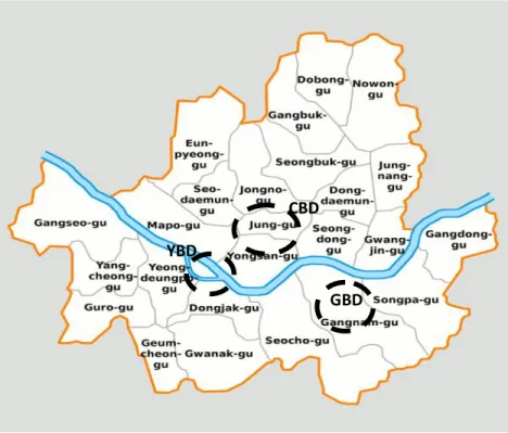
Seoul is the capital and largest city of South Korea. A megacity with a population of over 10 million, it is one of the largest cities in the world. The Seoul National Capital Area is the world's second largest metropolitan area with over 24.5 million inhabitants, which includes the Incheon metropolis and most of Gyeonggi province. Almost half of South Korea's population lives in the Seoul National Capital Area, and nearly a quarter in Seoul itself, making it the country's foremost economic, political, and cultural center. Seoul is divided into 25 Gu (district). 13The Gu vary greatly in area (from 10 to 47 km²) and population (from less than 140,000 to 630,000). Songpa has the most people, while Seocho, the largest area. The government of each Gu handles many of the functions that are handled by city governments in other jurisdictions. Each Gu is divided into dong, or neighborhoods
Fig 2 Seoul City Map
13 As of Feb. 2008 CBD YBD GBD
20
The Seoul office market has three major submarkets: 1) CBD (Central Business District), 2) GBD (Gangnam Business District) and 3) YBD (Yeouido Business District)14. They account for 70 percent of large office buildings with 30,000 sqm or more total area: 35.9 percent of total office space is located in CBD, 24.0 percent in GBD and 13.4 percent in YBD.
CBD is the oldest and the largest business district developed in the 1960‟s, followed by GBD, and then YBD. The CBD is still the most preferred location for MNCs15 and Chaebols because of tradition and well-established support facilities. Foreign banks, securities houses, embassies, and consulting companies dominate the CBD.
The Central Government designated GBD, formerly an agricultural area, as the second business district of Seoul. In the middle 1990‟s, GBD gained popularity centering around Gangnam Rd. and Teheran Rd. as the IT valley of Seoul and the “Teheran Valley.” After 1998, GBD showed rapid rent hikes and eventually followed the rent level up with that of CBD.
In the late 1970‟s through the early 1980‟s, development in YBD was encouraged as the „Manhattan of Seoul.‟ YBD remains the center of securities trading and broadcasting activities. Local securities, media, and IT companies dominate the district due to its close proximity to the Korea Stock Exchange, broadcasting stations, and the Yongsan Electronic Market.
14
Description of three submarkets is referred to in CBRE’s quarterly report. 15
21 3.2. Historical Trends of Seoul Office Market
3.2.1 Rent
Rent Index
For this study, a Seoul office rent index 16 for 36 years (from 1975 to 2010) was developed by the author by combining the rent data from the study by Park (1999) and Shinyoung 17. Then the real
(inflation-adjusted) rent index was constructed from the constant value based on 100 in 2005.
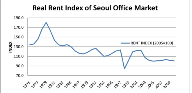
Fig 3 Source : Refer to the text
In the index for the last 36 years, the highest rent was 180.3 in 1979. While this high rent can hardly be explained by any economic reason, the driving factor might be the mental impact caused by the new governmental policy. According to Choi (1993), from 1977 to the early 1980s, the government
16 Refer to Section 4.1 for the detailed methods for the development of the index 17
Shinyoung is a Korean real estate service and development company that maintains a comprehensive database for the Seoul office market.
70.0 90.0 110.0 130.0 150.0 170.0 190.0 INDE X
Real Rent Index of Seoul Office Market
22
prohibited all new development north of the Han River, which included the major office district, for purposes of decentralization of Seoul and national defense. Therefore, rents steeply increased in the beginning of this period (in 1978 and 1979), but soon it fell to a normal level. On the other hand, rent hit the bottom (84.2) in 1998, due to the Asia Debt Crisis. In 1998, the Korea economy shrank at an unexpected rate, unemployment rate rose to 6.7%, an increase of 61.7% from previous year, and the GDP growth rate was -6.9%18. In this situation, with skyrocketing vacancy rate, rent decreased dramatically; however, it soon recovered and remained stable until 2003. Currently, the Seoul office market has one of the most expensive rents in the world.19
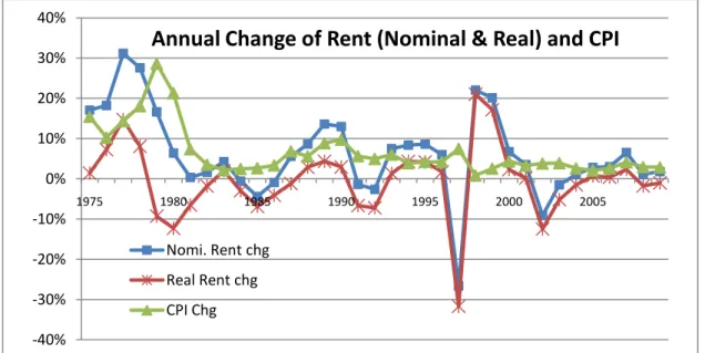
Fig 4 Source: Bank of Korea (CPI) and the author (rent)
According to Fig 2.4, we can see the cyclical movement of the annual change in the rent. During the period studied, there were six peaks with six-year cycles and the cycle of the 1994-2000 period was noticeably greater than that of others. Nominal rent increased on average six percent annually;
18
According to the Bank of Korea, the GDP growth rate of Korea from 1997 to 2000 was 4.7%, -6.7%, 9.5% and 8.5% respectively.
19
According to the CBRE’s Global Office Rents survey on May 2010, Seoul CBD placed 5th most expensive rent in the Asia Pacific region and 21st in the world
-40% -30% -20% -10% 0% 10% 20% 30% 40% 1975 1980 1985 1990 1995 2000 2005
Annual Change of Rent (Nominal & Real) and CPI
Nomi. Rent chg Real Rent chg CPI Chg
23
however, real rent decreased -0.4% annually during the given periods. Rent showed a strong
correlation with the CPI before 1998, but after 1998, even though the CPI was stable, rent fluctuated20.
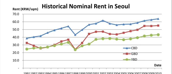
Fig 5 Source: Shinyoung
In Fig 2.5, based on Shinyoung’s historical rent data from 1991 to 2010, CBD has the highest rent among the three major submarkets of Seoul; however, all of them have almost the same trends. This shows that, even though there are differences in tenant profile, location, and vacancy rate, the rents of three major submarkets of Seoul are affected by same factors.
Lease Structure
Historically, it has been very difficult for developers or investors to secure long-term financing for either property acquisition or development in Korea. Even when it is secured, the loan to value (LTV) ratio typically does not exceed 50 percent of the property's appraised market value. With limited
20
The correlation between rent and CPI was 42.7% during 1975-2010, but 62.5% during 1975-1997. -10.0 20.0 30.0 40.0 50.0 60.0 70.0 19911992199319941995199619971998199920002001200220032004200520062007200820092010 Rent (KRW/sqm) Date
Historical Nominal Rent in Seoul
CBD GBD YBD
24
financing options, they usually turn to the commercial leasing market to cover their financing obligations. There are two prevailing lease structures in the office leasing market.
The first leasing structure is that tenants make one single deposit payment prior to occupation of the premises, which is refunded without interest to the tenants in full upon expiration of the lease. This is the so-called Chonsei, and under this system, the tenant is not liable for monthly rent. The imputed rent is the interest (or investment return) for the deposit earned by the landlord during the term of the lease.
Another prevailing lease structure is that tenants make a combination of a one-time deposit and a monthly rent payment, or the Walsei with Deposit system. The deposit is returned upon expiration of the lease. Generally, the amount of deposit is ten months of rent. However, Heo (1998) found that the ratio of deposit amount to monthly rent varies according to the office sub-markets and the type of owners. His study showed that the average ratio of deposit is 14 months of rent among three dominant Seoul office sub-markets.
According to the survey of the KRERI21 (as of 4Q 2010), the Walsei with Deposit system accounts for 91.20 percent of office leases and the Chonsei system accounts for 4.30 percent. The latter is
continuously decreasing because landlords want to avoid interest rate risk instead of maximizing leverage effects due to low market interest rate.
Chonsei Walsei (Monthly) Only Walsei with Deposit
2008 6.70% 2.10% 91.20%
2009 4.20% 2.40% 93.40%
2010 4.30% 1.50% 94.20%
Fig 6 Source: KRERI
21
Korea Real Estate Research Institute (KRERI) publishes quarterly reports about the Korea commercial real estate market (office and retail).
25 Lease Term
The lease term is simply the length of a lease. According to the KRERI, as of 4Q 2010, the average lease term of Seoul office is 19.3 months, which is less than 2 years. Although the office lease length in Seoul has significantly increased from early 1980, it is still much shorter than in the U.S.22
The recent trend toward a longer lease term is desirable for a number of reasons. Both owners and tenants can reduce risk from severe future rent fluctuation, which will help owners get permanent financing for their buildings as they will have more concrete future cash flows to be appreciated by lenders. Both owners and tenants also benefit from the reduction in costs and time of the re-negotiation of the lease or the extensive search for a new office. If the average lease length were, for example, two years, then half of all leases would expire each year, creating quite a large pool of tenants who
potentially might move.
3.2.2 Supply of Office Space
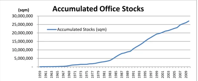
For the last 50 years, the Seoul office market has experienced an explosive growth. According to
Shinyoung, by end of 2010, the total space of office buildings over 9 stories in Seoul reached 27
million square meters representing a dramatic increase – 4,725 times from a mere 5,719 square meters in one building in 1959. For 51 years, office space over 9 stories has grown 17.7% annually.
22
26
Fig 7 Source: Shinyoung
Fig 8 Source: Shinyoung
In Fig 8, the cyclical movement of the growth of new office supply can be observed. During 40-year period from 1961 to 2010, there were five peaks in 1970, 1979, 1984, 1992 and 2007. The peak in 1984 can be mainly explained by the high rent period from 1978 to 1980, given the long lead-time for planning and construction of office buildings. The peak in 1992 can be explained by the impact of a new tax law. According to Choi (1995), the supply of office spaces burgeoned, especially in Kangnam Area where there lay many vacant lots, in anticipation of the government imposing land value
-5,000,000 10,000,000 15,000,000 20,000,000 25,000,000 30,000,000 1959 1961 1963 1965 1967 1969 1971 1973 1975 1977 1979 1981 1983 1985 1987 1989 1991 1993 1995 1997 1999 2001 2003 2005 2007 2009
(sqm)
Accumulated Office Stocks
Accumulated Stocks (sqm) 0.0% 10.0% 20.0% 30.0% 40.0% 50.0% 60.0% 70.0% 80.0% 1961 1963 1965 1967 1969 1971 1973 1975 1977 1979 1981 1983 1985 1987 1989 1991 1993 1995 1997 1999 2001 2003 2005 2007 2009
Annual New Supply as a Percent of the Stock of Office Space
27
increment tax 23 as of January 1990. Due to the Debt Crisis during 1997-1998, many Korean
developers and companies canceled or delayed office construction because of weaker demand, which result in limited supply until 2007. In 2007, extremely low vacancy rate because of insufficient office space attracted many developers and corporations with robust economic growth to build office buildings in Seoul.
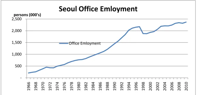
3.2.3 Office Employment
Although the only data available for Seoul office employment before 1990 is from a population census conducted every 5 years, they become available since 1990 from the Annual Report on the
economically Active Population Survey conducted by the National Statistical Office of Korea. Therefore, office employment data in Seoul before 1990 are estimated using the whole country's data.24
As seen in Fig 10, office employment in Seoul experienced a severe downturn in 1972, 1981, 1998 and 2010 when there was significant negative economic shock in Korea and Seoul., In 1998, especially, office employment of Seoul was -13.5% because of the negative economic shock of the Debt Crisis. Recently, after the global credit crisis in 2008, the office employment growth of Seoul turned negative for the first time since 1998; however, it recovered faster than other countries like the U.S., and expectation and long-term growth of the office employment has been more stable in the 2000s than before.
23
This tax targets vacant or under-utilized land to reduce land speculation. The land value increment tax imposes high tax rates (30 - 50%) on any gains from excessive land price appreciation of idle land. The tax base or excessive gain is the appreciated price of the land minus the national average land price
appreciation and any necessary expenses for land improvement. The land price calculation is based on the
Gong-Si-Ji- Ga, an appraised standard land price, announced by the Ministry of Construction and
Transportation. The tax period is 3 years, starting from January 1990. A taxpayer can obtain a tax credit for land price depreciation during previous tax periods. (Park (1999)
24
Park (1999) calculated office employment data of Seoul before 1990 assuming that office employment both in Seoul and in all of Korea tended to grow at the same rate. Therefore, the annual growth of office
employment in Seoul before 1990 was estimated from that of national data. Refer to Chapter 4 for detailed methodology.
28
Fig 9 Source: Park (1999), National Statistics Office of Korea
Fig 10 Source: Park (1999), National Statistics Office of Korea
-500 1,000 1,500 2,000 2,500 1966 1968 1970 1972 1974 1976 1978 1980 1982 1984 1986 1988 1990 1992 1994 1996 1998 2000 2002 2004 2006 2008 2010
persons (000's)
Seoul Office Emloyment
Office Emloyment -20.0% -15.0% -10.0% -5.0% 0.0% 5.0% 10.0% 15.0% 20.0% 25.0% 30.0% 1967 1969 1971 1973 1975 1977 1979 1981 1983 1985 1987 1989 1991 1993 1995 1997 1999 2001 2003 2005 2007 2009
Seoul Office Employment Growth
Seoul Office Employment Growth
29 3.2.4 Vacancy Rate
According to DiPasquale and Wheaton (1996), vacancy is a period through which parcels of space within buildings pass either as they wait to be rented for the first time or become available after a tenant moves out. Since 1991, Shinyoung has included vacancy rate of over 9 stories buildings as one of their annual survey items. Even though the length of the vacancy rate data period is relatively shorter than that of rent or office supply, vacancy rate can be used as a meaningful indicator for the recent change in the Seoul office market.
In Fig 11, the vacancy rate of the Seoul office market increased rapidly to 19.1 percent in 1998 because of the continuing of large supply of the past few years and decreased demand triggered by the debt crisis. However, as the Korea economy recovered, the vacancy rate of 2000 decreased very dramatically to 2.7%, and then, due to limited supply, the office vacancy rate of Seoul has been very stable and kept a low level.
<Fig 11> Source: Shinyoung (Vacancy rate of 2011 is as of Q1) 0.0%
5.0% 10.0% 15.0% 20.0%
25.0%
Vacancy Rate of Seoul Office
CBD GBD YBD Average
30
Recently, the vacancy rate of YBD has been the lowest among three submarkets because of few office spaces and strong demand from financial firms such as securities companies and asset management companies.
3.2.5 Cap Rate
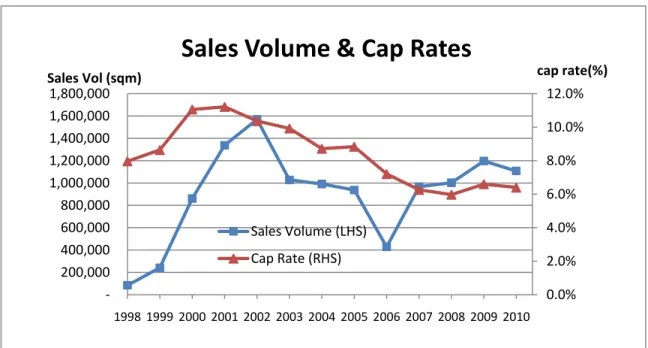
Since 1998, Shinyoung has been collecting information on actual office sales transactions in Seoul and in Korea. Between 1998 and 2010, Shinyoung data spans 468 transaction records in Seoul and Fig 12 shows historical sales volume and cap rates in the city.
Fig 12 Source: Shinyoung
In Fig 12, it can be seen that cap rates in Seoul keep moving down even though sales volume is volatile and there was a global credit crisis that affected Korea as well. There are two reasons that explain this strong cap rates movement: (1) There is not enough office space in Seoul, especially above class A level, meaning that buyers do not have enough options to negotiate price. (2) After 2000,
0.0% 2.0% 4.0% 6.0% 8.0% 10.0% 12.0% -200,000 400,000 600,000 800,000 1,000,000 1,200,000 1,400,000 1,600,000 1,800,000 1998 1999 2000 2001 2002 2003 2004 2005 2006 2007 2008 2009 2010 cap rate(%) Sales Vol (sqm)
Sales Volume & Cap Rates
Sales Volume (LHS) Cap Rate (RHS)
31
investors that purchase office buildings increased and diversified, like REITs, REF, pension funds and foreign investors. Thus, this inflow of investors resulted in competition, which have raised prices due to limited supply.
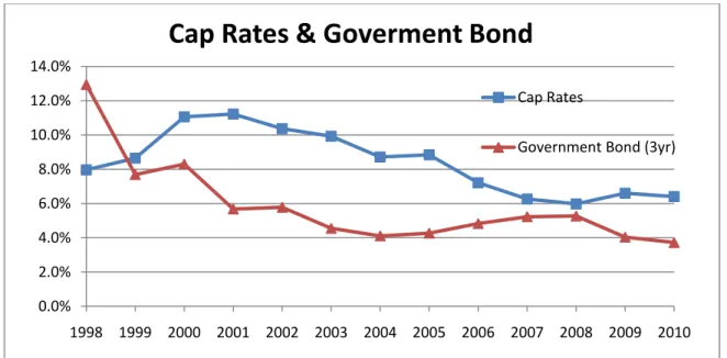
Fig 13 Source: Shinyoung
The cap rate spread is the difference between market cap rates and the risk free rate, usually the Treasury rate25. Since the Treasury rate represents the risk-free rate, the capitalization rate has spread, which in essence reflects the risk premium real estate investors required in order to invest in real estate. In Fig 13, cap rate spreads were low until 2008, with the recent peak of real estate market; after that, the spread began to widen. 26
25 Unlike U.S., which usually uses 10 year Treasury Bonds, 3 year government bonds are the most common indicator of the risk free rate in Korea.
26
The spread was 0.7% in 2008, and 2.7% in 2010. 0.0% 2.0% 4.0% 6.0% 8.0% 10.0% 12.0% 14.0% 1998 1999 2000 2001 2002 2003 2004 2005 2006 2007 2008 2009 2010
Cap Rates & Goverment Bond
Cap Rates
32
CHAPTER 4. ECONOMETRIC MODEL FOR SEOUL OFFICE MARKET
4.1. Data Set Used in the Study
4.1.1 Rent Index
To construct a historical office rent index, two different sources are used for this thesis: rent data from
Shinyoung and the study by Park (1999). Shinyoung has published quarterly surveyed rental rates and
other related items for offices in Korea since 1991. As of the end of 2010, they have collected data from 880 office buildings in Seoul which are over 9 stories or have more than 6,600 square meters of total gross area; there are 234 buildings in CBD, 308 in GBD, 151 in YBD, and 187 in other areas in Seoul. In his study, Park (1999) collected office rent from the Korea Chamber of Commerce and Industries (KCCI) and the study of Um (1988)27.
After examining periods in which two data sets are duplicated, two things have been found: (1) First of all, the two data sets show same trend, which increased 28.7% from 1991 to 1997, and (2) Shinyoung’s data is 62-75% of Park‟s data. Based on these findings, Shinyoung’s office rent extends to before 1991, assuming that Shinyoung’s rent data is 72% of Park‟s data. As a result, historical nominal rent from 1975 to 2010 has been assembled.
After estimating the historical annual rental costs for 36 years, they have been discounted according to the Consumer Price Index (CPI) to adjust for inflation. Finally, the real rental index has been
constructed from the constant value of annual rents, based on 100 in 2005.
27
The KCCI has annually surveyed rental rates and other lease-related items for office and commercial property in Seoul since 1985. In most surveys, it interviewed 150 rented offices comprised of 6 offices in all 25 Gus - two each from high, medium, and low-grade offices. In her study, Um (1988) has collected the office rent data from 1974 to1988.
33 4.1.2 Supply of Office Space
Shinyoung has assembled annual completion data for office buildings over 9 stories in Seoul since 1959.
In this thesis, this data ws used for historical supply of Seoul offices. In addition, to forecast the Seoul office market with planned big supplies for next few years, the future completion of office space from 2011 to 2016 from Shinyoung’s estimation was used.
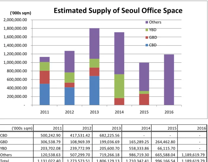
Fig 14 (above), Fig 15 (below) Source: Shinyoung
-200,000.00 400,000.00 600,000.00 800,000.00 1,000,000.00 1,200,000.00 1,400,000.00 1,600,000.00 1,800,000.00 2,000,000.00 2011 2012 2013 2014 2015 2016
('000s sqm)
Estimated Supply of Seoul Office Space
Others YBD GBD CBD ('000s sqm) 2011 2012 2013 2014 2015 2016 CBD 500,242.90 417,531.42 682,225.56 - - -GBD 306,538.79 108,969.39 199,036.69 165,289.25 264,462.80 -YBD 203,702.08 239,772.99 205,600.70 558,333.86 66,115.70 -Others 120,538.63 507,299.70 719,266.18 986,719.30 665,588.04 1,189,619.79 Total 1,131,022.40 1,273,573.51 1,806,129.13 1,710,342.41 996,166.54 1,189,619.79
34
According to the Fig 14 and 15, more than 8.1 billion square meters, an average of 1.3 billion square meters annually, are going to be delivered to Seoul office market, accounting for 30% of existing office space in Seoul.28 In this study, this estimation for exogenous supply for forecasting has been used.
4.1.3 Office Employment
Although the only data available for Seoul office employment before 1990 is from a population census conducted every 5 years, they become available since 1990 from the Annual Report on the
Economically Active Population Survey conducted by the National Statistical Office of Korea.29 Therefore, in this thesis, two data sets for office employment of Seoul are used; one is the Annual Report on the Economically Active Population Survey since 1990, and the other is Park‟s (1999) data, calculated from office employment data in Korea which has been available since 1963.
Park 1999) used the following equations to estimate office employment of Seoul before 1990, based on the assumption that office employment both in Seoul and all of Korea tends to grow at the same rate.
28 As of 2010, the office space stock in Seoul is 27b square meter. (from Shinyoung) 29
The National Statistical Office of Korea publishes its Annual Report on the Economically Active Population
Survey, which contains data for employment by occupation and by industry. The annual data for Seoul
office employment for this study are estimated by adding three categories in the employment by occupation section: 1) legislators, senior officials, and managers; 2) professionals, technicians, and associate
35 4.1.4. Vacancy Rate
Shinoung’s historical annual vacancy rate of Seoul offices from 1991 to 2010 was used as the data of
vacancy rate in this thesis. Because historical vacancy rate data has been available only since 1991, while other data such as rent, office supply, and office employment has been available since 1975, the two models, that is, the full model with vacancy rate and the simple model without vacancy rate, have been used in this thesis.
4.2. Econometric Models
4.2.1 Simple Model
As stated in the above chapters, in this thesis, two models for investigating office market have been used; one is the simple model with vacancy rate, the other is the full model with vacancy rate. Whereas the simple model has a longer data period, making for more stable and reliable equations, it lacks an absorption equation which represents demand.
4.2.1.1 Rent Equation
In the market for office use or space, demand comes from the occupiers of space, whether they are tenants or owners. The cost of occupying space is the annual outlay necessary to occupy or use the property, or its rent. For tenants, rent is simply an annual rental payment plus the opportunity (or interest) costs of a deposit, if any, as specified in a lease agreement. For owners, rent is defined as the annualized cost associated with the ownership of properties.
36
Rent is determined by the intersection of the demand for space use and the supply of space. All else being equal, when the number of employees increases, the demand for space rises, which raises the rent as well. With fixed demand, when new offices are supplied in the market, the rent declines. On the other hand, the level of rent influences both the demand and the supply for space as well. All else being equal, if the rent rises (or falls), the occupiers of space or firms reduce (or expand) the space per worker, and thus the demand for space decreases (or increases). Similarly, if the rent rises, the supply of new office buildings increases slowly because of the long lead-time for planning and construction. However, even though the rent falls, the new supply cannot be less than zero.
As rent is determined by the demand and supply, it can be expressed by the function of immediate past and current real Gross Domestic Product (GDP), GDPt and GDPt-1, stock of space, S, and the immediate past rent, Rt-1. The immediate past rent is included here as an independent variable since it is the base for the negotiation of rent, and thus influences the current rent. Current and past GDP are used for a proxy for demand.
Rt = α0+ α1 St + α2 GDPt + α3 GDPt-1+ α4 Rt-1 ……..(1)
Fig 16 Summary of the Regression Analysis for Rent Equation (Simple model) Regression Statistics Multiple R 0.919886 R Square 0.84619 Adjusted R Square 0.825681 Standard Error 1.179391 Observations 35 Coefficients Standard
Error t Stat P-value
Intercept 39.19497 3.014719 1.793619 0.082961 St -6.2E-06 3.81E-07 -2.24305 0.032433 GDPt 0.000349 1.16E-05 4.149582 0.000253
37
GDPt-1 -0.0002 1.21E-05 -2.24975 0.031957 R t-1 0.674834 0.147714 4.568526 7.85E-05
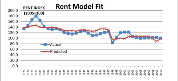
The estiated equation suggests that rent seems to be fully explained by the immediate past rent, current and one year lagging GDP, and current office stock in the Seoul economy. Since the prevailing lease term in Seoul is less than two years and most of the tenants can thus move to other buildings providing
competitive rent, building owners in Seoul may be forced to immediately adjust rents based on the GDP, which represents demand, and the stock of office space. When the office stock increases (decreases) one percent, and all else is equal, the rent decreases (increases) 0.1 percent. On the other hand, when the current GDP increases one percent, and all else is equal, the rent increases 0.2 percent.
Fig 17 Source: Author‟s analysis
4.2.1.2 Construction Equation
There are two types of investors for the construction of office buildings: developers (speculators) and owner-occupiers. Each of them has a different motive for his decision to construct office buildings. While
0.0 20.0 40.0 60.0 80.0 100.0 120.0 140.0 160.0 180.0 200.0 1976 1977 1978 1979 1980 1981 1982 1983 1984 1985 1986 1987 1988 1989 1990 1991 1992 1993 1994 1995 1996 1997 1998 1999 2000 2001 2002 2003 2004 2005 2006 2007 2008 2009 2010 RENT INDEX (2005=100)
Rent Model Fit
Actual Predicted
38
developers consider the return on the investment, or rent, owner-occupiers consider adequate working space for their employees.
As the investment decision is influenced by rent and space needs, the annual new supply or completion of office buildings can be expressed by the function of the past rents, Rt-n and Rt-n-1, which lag (t) and (t-1) years, growth of past real GDP, GGDPt-n , and past completion, Ct-n. Among several sets of lagging rent and employment growth, the following equation has the best statistical fit.
Ct = α0+ α 1Ct-1+ α2Rt-5+ α3Rt-6+ α4GGDPt-2 ………..(2)
Fig 18 Summary of the Regression Analysis for Completion Equation (Simple model) Regression Statistics Multiple R 0.412383295 R Square 0.170059982 Adjusted R Square 0.037269579 Standard Error 353910.3203 Observations 30 Coefficients Standard
Error t Stat P-value
Intercept 333413.6337 488206.783 1.02091 0.474061 Ct-1 0.364487288 0.20078082 1.80598 0.09117 Rt-5 11723.39559 6217.05166 1.30455 0.771044 Rt-6 -9339.6097 6379.05652 -1.0554 0.849884 GGDPt-2 1646144.337 1398542.49 1.22324 0.521389
The estimated equations suggest that new office supply can be explained by five and six years lagging rents, two year lagging GDP growth, and immediate past completion. This lag can be explained primarily by the long-lead time needed to plan and construct office buildings. Another explanation is the delay of reporting (information) in the market, since information for the Seoul office market is not immediately available and acute information is costly to obtain. Furthermore, the equation implies that investors,
39
whether developers or owner-occupiers, have expected current conditions to prevail in the future - a myopic expectation. This myopic expectation can generate market volatility since by the time space enters the stock, market conditions may have changed.
Also, relatively low R square can be explained by political or other decisions, not directly connected to market conditions, to influence office completion.
Fig 19 Source: The author
4.2.1.3 Identity Equation
To complete the model, we need an identity equation that explains the relationship between stock and new supply or completion. The following equation explains that the stock of total space in each period, St, is updated from that of the previous period with new space deliveries or completions.
St = St-1 + Ct
Using the equations of rent and construction as well as the above identity equation, variables for each period will be given by the conditions of the preceding periods.
-200,000.00 400,000.00 600,000.00 800,000.00 1,000,000.00 1,200,000.00 1,400,000.00 1,600,000.00 1,800,000.00 1981 1982 1983 1984 1985 1986 1987 1988 1989 1990 1991 1992 1993 1994 1995 1996 1997 1998 1999 2000 2001 2002 2003 2004 2005 2006 2007 2008 2009 2010
sqm
Completion model Fit
Predicted Actual
40 4.2.2 Full Model with Vacancy Rate
According to Wheaton and DiPasquale (1996), vacancy is a period through which parcels of space within buildings pass either as they wait to be rented for the first time or become available after a tenant moves. In the commercial market, movements of fluctuations in vacancy are far more pronounced and persist for many periods. This suggests that rents or prices are not clearing the market, and that demand must be measured distinct from supply – that is to say, demand is measured as the amount of occupied space, whereas supply is the sum of occupied and vacant space. In this methodology, vacancy rate has the critical role of estimating supply and demand by calculating occupied stock.30
Based on Wheaton‟s model, data from 1991 to 2010, which includes vacancy rate, is used for making three equations: (1) the rent equation, (2) the supply equation, and (3) the demand, or absorption equations.
4.2.2.1 Rent Equation
In a rental market, the risk of vacancy lies mainly with the landlord, so that greater vacancy and fewer relocating tenants raise the expected leasing time, and hence lower the minimum rent that landlords are willing to accept. On the tenant‟s side of negotiation, when there are few other searching tenants and much vacant space, it becomes easier to find appropriate new space. Thus, the maximum rent the tenant is willing to offer will be less when vacant space is plentiful. Both of these move inversely with vacancy.
Considering above simple relationships between vacancy and rents, following equation is to be constructed.
30
41 Rt = α0+ α1 Rt-1 +α2 Vt + α3 Vt-1……….(3)
Fig 20 Summary of the Regression Analysis for Rent Equation (Full Model)
Regression Statistics Multiple R 0.697483 R Square 0.486482 Adjusted R Square 0.383778 Standard Error 1.157086 Observations 19 Coefficients Standard
Error t Stat P-value
Intercept 32.24685 26.12092 1.234522 0.235999 Rt-1 0.723992 0.230971 3.134554 0.006818 Vt -204.675 67.35611 -3.0387 0.008292 Vt-1 145.646 73.13279 1.991528 0.064955
In Equation (3) above, rent can be determined as a linear function of immediate past rent, Rt-1, current and one year lagging vacancy rate, Vt and Vt-1. Rent is influenced positively by past rent and negatively by the change of vacancy rate; in other words, if vacancy rate goes up, rent will go down.
Equation (3) is modified as following : R – R-t = α x (R* - Rt-1)
Rt-Rt-1 =0.27601 x (116.833-741.5551 Vt+527.687 Vt-1)-0.27601 Rt-1
R* = 116.833-741.5551 Vt+527.687 Vt-1
Using the historical average for vacancy rate (Vt=Vt-1=0.05), equation (4) implies that real rents will head toward 106.14. With the vacancy near 10 percent, the real rent index will move toward a level of only 95.45.
42
Fig 21 Source: The author
4.2.2.2 Supply Equation
As mentioned above in chapter 4.2.1.2, myopic expectations, which developers have when they expect current conditions to prevail in the future, can lead to severe and repeated market oscillations. On the other hand, even rational expectations will generate a single market cycle in the presence of long construction lags. If there is a sudden change in office demand (e.g., increase in office employment), rationally based construction eventually will build just the right amount of additional space. Even though fully anticipated, the lagged timing of this new supply cannot be avoided.
In equation (4), office completion can be explained by a four year lagging vacancy rate, a five year lagging rent, and immediate past completion. The difference lag time between rent and vacancy would be caused by the fact that it is harder to get current rent data than vacancy rates.
Ct = α0 + α1Ct-1+α2Rt-5+α3Vt-4 ……….(4)
Fig 22 Summary of the Regression Analysis for Supply Equation (Full Model) Regression Statistics 0 20 40 60 80 100 120 140
Real Rent Index
Rent Model Fit - Full model
Predicted Actual
43 Multiple R 0.543187 R Square 0.295052 Adjusted R Square 0.118815 Standard Error 328995 Observations 16 Coefficients Standard
Error t Stat P-value
Intercept -575381 847508.1 -0.67891 0.510078 Ct-1 0.120549 0.247698 0.486677 0.635255 Rt-5 12472.66 7376.668 1.690826 0.116655 Vt-4 -1941127 1794603 -1.08165 0.300667
As a result, annual office completion is impacted positively by past rent and previous completion, and negatively by past vacancy rate. The implications of this model are easy to interpret. At the recent twenty-year average of rent (109.7) and vacancy rate (5.0%), 791,397 square meters of new office supply will be completed. If rent increases (decreases) 1.0%, completion after 5 years increases (decreases) 0.02%.
Fig 23 Source: The author
0 200000 400000 600000 800000 1000000 1200000 1400000 1600000 1800000 1995 1996 1997 1998 1999 2000 2001 2002 2003 2004 2005 2006 2007 2008 2009 2010
(sqm)
Supply Model Fit - Full model
Predicted Actual
44 4.2.2.3 Demand Equation
Considerale evidence indicates that the primary instrument driving office space demand is employment in selected sectors of an economy (DiPasquale and Wheaton 1995). The actual demand for offices can be measured, ex post, as the amount of office space occupied, out of that existing in the total stock. To model net absorption or the change in occupied space, let OC represent the amount of space that all firms in the market would in principle demand if there were no leases, moving, or adjustment cost to obtaining such space. Usually, market demand for office space should be the product of the number of office workers and recent rent,31 however, even if office employment is increasing, absorption would be decrease when office space for workers is decreasing. So, in this study, I added GDP per employment instead of the number of employment because it can be good indicator for space per worker movement. If GDP per employment is going up, it means that the productivity of workers is increasing, so that firms will increase office workers and space for them.
AB = α0+ α1 OC t-1 + α2 GDPt + α3 GDPEMPt + α4Rt-1………….(5)
Fig 24 Summary of the Regression Analysis for Demand Equation (Full model) Regression Statistics Multiple R 0.75962115 R Square 0.57702429 Adjusted R Square 0.45617409 Standard Error 536114.813 Observations 19 Coefficients Standard
Error t Stat P-value
Intercept 5825205.16 2666551 2.184547 0.046424 OC t-1 -0.18911715 0.219697 -0.86081 0.403846
31
Wheaton et al. (1997) constructed equation for ABt = 0.25 X [7.3+Et(294.8-0.92Rt-1)]-0.25OSt-1 of the London office market demand.
45
GDPt 2.04419021 6.496798 0.314646 0.757671 GDPEMP 4984.55334 4389.206 1.135639 0.275176 RRENT(t-1) -43728.4032 15948.77 -2.7418 0.015899
In equation (5), absorption can be well explained by the linear function of GDP, GDP per office employment (GDPEMP), immediate past rent, and immediate past occupied stock. In other words, absorption is positively affected when GDP and GDP per employment, and negatively by recent rent and previous occupied stock.
Fig 25 Source: The author
4.2.2.4 Identity Equation
In this chapter, my approach to modeling commercial space begins with three accounting identities. First, the stock of total space in each period, St, is updated from that of the previous period with new space deliveries or completions, Ct. This stock-flow equation, Equation (6), is no different from that in Chapter 4.2.1.3. Next, the demand for office space at any time can be measured ex post as the portion of office stock that is actually consumed or occupied, OCt. This involves defining the vacancy rate, Vt, as
-500,000 0 500,000 1,000,000 1,500,000 2,000,000 2,500,000 3,000,000 1992 1993 1994 1995 1996 1997 1998 1999 2000 2001 2002 2003 2004 2005 2006 2007 2008 2009 2010
(Sqm)
Demand (Absorption) Model Fit - Full model
Predicted Actual
46
the percentage difference between the total stock and the occupied stock, Equation (7). Finally, the net absorption of office space, ABt, is defined as the change in the amount of occupied office space from period to period. This, in Equation (8) the current amount of occupied space, OCt, equals that of the previous period plus the net space absorption, ABt. Net absorption is positive when existing vacant space is leased, or when newly built office space is leased without increasing the vacancy of existing buildings. These three relationships are accounting identities, rather than behavior economic theories.
St = St-1 + Ct ………..(6) Vt = (St-OCt)/St ...(7) OCt = OCt-1 + ABt ………..(8)
4.3 Limits of the Model
4.3.1 Ignorance of the Interrelationship with Adjacent Cities
Since Seoul forms a huge metropolitan area with surrounding cities such as Inchon and other satellite cities, the economic area might be bigger than the municipal area of the city. Thus, the economic conditions of surrounding cities closely interact with those of Seoul, and they influence the economic variables (e.g., rent, new supply, stock, and employment) affecting the Seoul office market. For example, many employees working in Seoul live in bedroom suburbs and satellite cities located outside of the municipal area. On the other hand, employees living in Seoul do not necessarily work in the city. However, in this study, this interrelationship is ignored for the following reasons: (1) the economic boundary is not explicit and hard to define; and (2) the available data such as rent and new supply are collected based on the simple municipal boundary of Seoul.