arXiv:hep-ex/0604020v1 10 Apr 2006
V.M. Abazov,36 B. Abbott,76 M. Abolins,66 B.S. Acharya,29 M. Adams,52 T. Adams,50 M. Agelou,18 J.-L. Agram,19 S.H. Ahn,31 M. Ahsan,60 G.D. Alexeev,36 G. Alkhazov,40 A. Alton,65 G. Alverson,64 G.A. Alves,2 M. Anastasoaie,35 T. Andeen,54 S. Anderson,46 B. Andrieu,17 M.S. Anzelc,54 Y. Arnoud,14 M. Arov,53 A. Askew,50 B. ˚Asman,41 A.C.S. Assis Jesus,3 O. Atramentov,58 C. Autermann,21 C. Avila,8 C. Ay,24 F. Badaud,13 A. Baden,62 L. Bagby,53 B. Baldin,51 D.V. Bandurin,36 P. Banerjee,29 S. Banerjee,29 E. Barberis,64P. Bargassa,81P. Baringer,59 C. Barnes,44 J. Barreto,2J.F. Bartlett,51U. Bassler,17D. Bauer,44
A. Bean,59 M. Begalli,3 M. Begel,72 C. Belanger-Champagne,5 A. Bellavance,68 J.A. Benitez,66 S.B. Beri,27 G. Bernardi,17 R. Bernhard,42L. Berntzon,15 I. Bertram,43M. Besan¸con,18 R. Beuselinck,44 V.A. Bezzubov,39 P.C. Bhat,51 V. Bhatnagar,27 M. Binder,25C. Biscarat,43K.M. Black,63 I. Blackler,44G. Blazey,53F. Blekman,44 S. Blessing,50 D. Bloch,19K. Bloom,68U. Blumenschein,23 A. Boehnlein,51 O. Boeriu,56 T.A. Bolton,60 E. Boos,38
F. Borcherding,51G. Borissov,43K. Bos,34 T. Bose,78 A. Brandt,79 R. Brock,66 G. Brooijmans,71A. Bross,51 D. Brown,79N.J. Buchanan,50 D. Buchholz,54M. Buehler,82V. Buescher,23 V. Bunichev,38S. Burdin,51 S. Burke,46
T.H. Burnett,83 E. Busato,17 C.P. Buszello,44J.M. Butler,63S. Calvet,15J. Cammin,72S. Caron,34 W. Carvalho,3 B.C.K. Casey,78 N.M. Cason,56 H. Castilla-Valdez,33 S. Chakrabarti,29 D. Chakraborty,53 K.M. Chan,72 A. Chandra,49 D. Chapin,78 F. Charles,19 E. Cheu,46 F. Chevallier,14 D.K. Cho,63 S. Choi,32 B. Choudhary,28 L. Christofek,59 D. Claes,68 B. Cl´ement,19 C. Cl´ement,41Y. Coadou,5M. Cooke,81W.E. Cooper,51D. Coppage,59 M. Corcoran,81M.-C. Cousinou,15B. Cox,45 S. Cr´ep´e-Renaudin,14D. Cutts,78 M. ´Cwiok,30H. da Motta,2A. Das,63
M. Das,61 B. Davies,43 G. Davies,44 G.A. Davis,54 K. De,79 P. de Jong,34 S.J. de Jong,35 E. De La Cruz-Burelo,65 C. De Oliveira Martins,3 J.D. Degenhardt,65F. D´eliot,18M. Demarteau,51R. Demina,72P. Demine,18 D. Denisov,51
S.P. Denisov,39S. Desai,73 H.T. Diehl,51 M. Diesburg,51 M. Doidge,43 A. Dominguez,68H. Dong,73 L.V. Dudko,38 L. Duflot,16 S.R. Dugad,29 A. Duperrin,15J. Dyer,66 A. Dyshkant,53 M. Eads,68 D. Edmunds,66 T. Edwards,45 J. Ellison,49 J. Elmsheuser,25V.D. Elvira,51 S. Eno,62P. Ermolov,38J. Estrada,51H. Evans,55 A. Evdokimov,37
V.N. Evdokimov,39 S.N. Fatakia,63 L. Feligioni,63A.V. Ferapontov,60 T. Ferbel,72 F. Fiedler,25 F. Filthaut,35 W. Fisher,51 H.E. Fisk,51 I. Fleck,23 M. Ford,45 M. Fortner,53H. Fox,23 S. Fu,51 S. Fuess,51 T. Gadfort,83 C.F. Galea,35 E. Gallas,51E. Galyaev,56C. Garcia,72 A. Garcia-Bellido,83 J. Gardner,59 V. Gavrilov,37 A. Gay,19
P. Gay,13 D. Gel´e,19 R. Gelhaus,49 C.E. Gerber,52 Y. Gershtein,50 D. Gillberg,5 G. Ginther,72 N. Gollub,41 B. G´omez,8 K. Gounder,51 A. Goussiou,56P.D. Grannis,73 H. Greenlee,51 Z.D. Greenwood,61E.M. Gregores,4 G. Grenier,20Ph. Gris,13J.-F. Grivaz,16 S. Gr¨unendahl,51 M.W. Gr¨unewald,30 F. Guo,73 J. Guo,73G. Gutierrez,51
P. Gutierrez,76A. Haas,71 N.J. Hadley,62P. Haefner,25 S. Hagopian,50J. Haley,69 I. Hall,76 R.E. Hall,48 L. Han,7 K. Hanagaki,51 K. Harder,60A. Harel,72R. Harrington,64 J.M. Hauptman,58 R. Hauser,66J. Hays,54T. Hebbeker,21
D. Hedin,53 J.G. Hegeman,34 J.M. Heinmiller,52 A.P. Heinson,49 U. Heintz,63 C. Hensel,59 G. Hesketh,64 M.D. Hildreth,56 R. Hirosky,82 J.D. Hobbs,73 B. Hoeneisen,12 M. Hohlfeld,16 S.J. Hong,31 R. Hooper,78 P. Houben,34 Y. Hu,73 V. Hynek,9 I. Iashvili,70 R. Illingworth,51A.S. Ito,51 S. Jabeen,63 M. Jaffr´e,16S. Jain,76
K. Jakobs,23C. Jarvis,62A. Jenkins,44 R. Jesik,44K. Johns,46 C. Johnson,71 M. Johnson,51A. Jonckheere,51 P. Jonsson,44 A. Juste,51 D. K¨afer,21 S. Kahn,74 E. Kajfasz,15 A.M. Kalinin,36 J.M. Kalk,61 J.R. Kalk,66 S. Kappler,21 D. Karmanov,38 J. Kasper,63 I. Katsanos,71 D. Kau,50 R. Kaur,27 R. Kehoe,80 S. Kermiche,15
S. Kesisoglou,78 A. Khanov,77 A. Kharchilava,70Y.M. Kharzheev,36D. Khatidze,71 H. Kim,79 T.J. Kim,31 M.H. Kirby,35B. Klima,51 J.M. Kohli,27 J.-P. Konrath,23M. Kopal,76 V.M. Korablev,39J. Kotcher,74 B. Kothari,71
A. Koubarovsky,38A.V. Kozelov,39 J. Kozminski,66 A. Kryemadhi,82 S. Krzywdzinski,51T. Kuhl,24A. Kumar,70 S. Kunori,62 A. Kupco,11T. Kurˇca,20,∗J. Kvita,9 S. Lager,41 S. Lammers,71G. Landsberg,78 J. Lazoflores,50 A.-C. Le Bihan,19P. Lebrun,20 W.M. Lee,53 A. Leflat,38F. Lehner,42 C. Leonidopoulos,71V. Lesne,13J. Leveque,46
P. Lewis,44J. Li,79 Q.Z. Li,51J.G.R. Lima,53 D. Lincoln,51J. Linnemann,66 V.V. Lipaev,39 R. Lipton,51 Z. Liu,5 L. Lobo,44A. Lobodenko,40M. Lokajicek,11A. Lounis,19P. Love,43H.J. Lubatti,83 M. Lynker,56 A.L. Lyon,51 A.K.A. Maciel,2 R.J. Madaras,47P. M¨attig,26 C. Magass,21 A. Magerkurth,65 A.-M. Magnan,14 N. Makovec,16
P.K. Mal,56 H.B. Malbouisson,3 S. Malik,68 V.L. Malyshev,36 H.S. Mao,6 Y. Maravin,60M. Martens,51 S.E.K. Mattingly,78 R. McCarthy,73 R. McCroskey,46D. Meder,24 A. Melnitchouk,67A. Mendes,15 L. Mendoza,8 M. Merkin,38K.W. Merritt,51A. Meyer,21J. Meyer,22M. Michaut,18 H. Miettinen,81 T. Millet,20J. Mitrevski,71 J. Molina,3N.K. Mondal,29 J. Monk,45 R.W. Moore,5T. Moulik,59 G.S. Muanza,16 M. Mulders,51M. Mulhearn,71 L. Mundim,3 Y.D. Mutaf,73E. Nagy,15M. Naimuddin,28M. Narain,63N.A. Naumann,35 H.A. Neal,65J.P. Negret,8
S. Nelson,50 P. Neustroev,40 C. Noeding,23 A. Nomerotski,51 S.F. Novaes,4 T. Nunnemann,25 V. O’Dell,51 D.C. O’Neil,5G. Obrant,40V. Oguri,3 N. Oliveira,3 N. Oshima,51 R. Otec,10 G.J. Otero y Garz´on,52M. Owen,45
G. Pawloski,81P.M. Perea,49 E. Perez,18 K. Peters,45P. P´etroff,16M. Petteni,44 R. Piegaia,1 M.-A. Pleier,22 P.L.M. Podesta-Lerma,33V.M. Podstavkov,51Y. Pogorelov,56M.-E. Pol,2A. Pompoˇs,76B.G. Pope,66A.V. Popov,39
W.L. Prado da Silva,3 H.B. Prosper,50 S. Protopopescu,74 J. Qian,65 A. Quadt,22 B. Quinn,67 K.J. Rani,29 K. Ranjan,28P.A. Rapidis,51 P.N. Ratoff,43 P. Renkel,80 S. Reucroft,64M. Rijssenbeek,73 I. Ripp-Baudot,19 F. Rizatdinova,77 S. Robinson,44 R.F. Rodrigues,3 C. Royon,18 P. Rubinov,51 R. Ruchti,56 V.I. Rud,38G. Sajot,14
A. S´anchez-Hern´andez,33 M.P. Sanders,62 A. Santoro,3 G. Savage,51 L. Sawyer,61 T. Scanlon,44 D. Schaile,25 R.D. Schamberger,73 Y. Scheglov,40 H. Schellman,54 P. Schieferdecker,25C. Schmitt,26 C. Schwanenberger,45 A. Schwartzman,69R. Schwienhorst,66 S. Sengupta,50 H. Severini,76 E. Shabalina,52M. Shamim,60 V. Shary,18 A.A. Shchukin,39 W.D. Shephard,56R.K. Shivpuri,28 D. Shpakov,64V. Siccardi,19R.A. Sidwell,60 V. Simak,10 V. Sirotenko,51P. Skubic,76 P. Slattery,72R.P. Smith,51 G.R. Snow,68J. Snow,75 S. Snyder,74S. S¨oldner-Rembold,45
X. Song,53 L. Sonnenschein,17A. Sopczak,43 M. Sosebee,79 K. Soustruznik,9M. Souza,2B. Spurlock,79 J. Stark,14 J. Steele,61 K. Stevenson,55 V. Stolin,37 A. Stone,52 D.A. Stoyanova,39J. Strandberg,41 M.A. Strang,70 M. Strauss,76R. Str¨ohmer,25 D. Strom,54M. Strovink,47L. Stutte,51 S. Sumowidagdo,50 A. Sznajder,3 M. Talby,15
P. Tamburello,46 W. Taylor,5 P. Telford,45 J. Temple,46 B. Tiller,25 M. Titov,23 V.V. Tokmenin,36M. Tomoto,51 T. Toole,62I. Torchiani,23 S. Towers,43 T. Trefzger,24S. Trincaz-Duvoid,17 D. Tsybychev,73B. Tuchming,18
C. Tully,69 A.S. Turcot,45P.M. Tuts,71 R. Unalan,66 L. Uvarov,40S. Uvarov,40 S. Uzunyan,53 B. Vachon,5 P.J. van den Berg,34 R. Van Kooten,55 W.M. van Leeuwen,34N. Varelas,52E.W. Varnes,46 A. Vartapetian,79 I.A. Vasilyev,39 M. Vaupel,26 P. Verdier,20L.S. Vertogradov,36M. Verzocchi,51 F. Villeneuve-Seguier,44 P. Vint,44
J.-R. Vlimant,17 E. Von Toerne,60 M. Voutilainen,68,† M. Vreeswijk,34 H.D. Wahl,50 L. Wang,62J. Warchol,56 G. Watts,83 M. Wayne,56 M. Weber,51 H. Weerts,66 N. Wermes,22 M. Wetstein,62 A. White,79 D. Wicke,26
G.W. Wilson,59 S.J. Wimpenny,49 M. Wobisch,51 J. Womersley,51 D.R. Wood,64 T.R. Wyatt,45 Y. Xie,78 N. Xuan,56 S. Yacoob,54 R. Yamada,51 M. Yan,62 T. Yasuda,51 Y.A. Yatsunenko,36K. Yip,74 H.D. Yoo,78
S.W. Youn,54 C. Yu,14 J. Yu,79 A. Yurkewicz,73 A. Zatserklyaniy,53C. Zeitnitz,26 D. Zhang,51 T. Zhao,83 Z. Zhao,65 B. Zhou,65 J. Zhu,73M. Zielinski,72 D. Zieminska,55 A. Zieminski,55 V. Zutshi,53 and E.G. Zverev38
(DØ Collaboration)
1Universidad de Buenos Aires, Buenos Aires, Argentina
2LAFEX, Centro Brasileiro de Pesquisas F´ısicas, Rio de Janeiro, Brazil
3Universidade do Estado do Rio de Janeiro, Rio de Janeiro, Brazil
4Instituto de F´ısica Te´orica, Universidade Estadual Paulista, S˜ao Paulo, Brazil
5University of Alberta, Edmonton, Alberta, Canada, Simon Fraser University, Burnaby, British Columbia, Canada,
York University, Toronto, Ontario, Canada, and McGill University, Montreal, Quebec, Canada
6Institute of High Energy Physics, Beijing, People’s Republic of China
7University of Science and Technology of China, Hefei, People’s Republic of China
8Universidad de los Andes, Bogot´a, Colombia
9Center for Particle Physics, Charles University, Prague, Czech Republic
10Czech Technical University, Prague, Czech Republic
11Center for Particle Physics, Institute of Physics, Academy of Sciences of the Czech Republic, Prague, Czech Republic
12Universidad San Francisco de Quito, Quito, Ecuador
13Laboratoire de Physique Corpusculaire, IN2P3-CNRS, Universit´e Blaise Pascal, Clermont-Ferrand, France
14Laboratoire de Physique Subatomique et de Cosmologie, IN2P3-CNRS, Universite de Grenoble 1, Grenoble, France
15CPPM, IN2P3-CNRS, Universit´e de la M´editerran´ee, Marseille, France
16IN2P3-CNRS, Laboratoire de l’Acc´el´erateur Lin´eaire, Orsay, France
17LPNHE, IN2P3-CNRS, Universit´es Paris VI and VII, Paris, France
18DAPNIA/Service de Physique des Particules, CEA, Saclay, France
19IReS, IN2P3-CNRS, Universit´e Louis Pasteur, Strasbourg, France, and Universit´e de Haute Alsace, Mulhouse, France
20Institut de Physique Nucl´eaire de Lyon, IN2P3-CNRS, Universit´e Claude Bernard, Villeurbanne, France
21III. Physikalisches Institut A, RWTH Aachen, Aachen, Germany
22Physikalisches Institut, Universit¨at Bonn, Bonn, Germany
23Physikalisches Institut, Universit¨at Freiburg, Freiburg, Germany
24Institut f¨ur Physik, Universit¨at Mainz, Mainz, Germany
25Ludwig-Maximilians-Universit¨at M¨unchen, M¨unchen, Germany
26Fachbereich Physik, University of Wuppertal, Wuppertal, Germany
27Panjab University, Chandigarh, India
28Delhi University, Delhi, India
29Tata Institute of Fundamental Research, Mumbai, India
30University College Dublin, Dublin, Ireland
31Korea Detector Laboratory, Korea University, Seoul, Korea
32SungKyunKwan University, Suwon, Korea
34FOM-Institute NIKHEF and University of Amsterdam/NIKHEF, Amsterdam, The Netherlands
35Radboud University Nijmegen/NIKHEF, Nijmegen, The Netherlands
36Joint Institute for Nuclear Research, Dubna, Russia
37Institute for Theoretical and Experimental Physics, Moscow, Russia
38Moscow State University, Moscow, Russia
39Institute for High Energy Physics, Protvino, Russia
40Petersburg Nuclear Physics Institute, St. Petersburg, Russia
41Lund University, Lund, Sweden, Royal Institute of Technology and Stockholm University, Stockholm, Sweden, and
Uppsala University, Uppsala, Sweden
42Physik Institut der Universit¨at Z¨urich, Z¨urich, Switzerland
43Lancaster University, Lancaster, United Kingdom
44Imperial College, London, United Kingdom
45University of Manchester, Manchester, United Kingdom
46University of Arizona, Tucson, Arizona 85721, USA
47Lawrence Berkeley National Laboratory and University of California, Berkeley, California 94720, USA
48California State University, Fresno, California 93740, USA
49University of California, Riverside, California 92521, USA
50Florida State University, Tallahassee, Florida 32306, USA
51Fermi National Accelerator Laboratory, Batavia, Illinois 60510, USA
52University of Illinois at Chicago, Chicago, Illinois 60607, USA
53Northern Illinois University, DeKalb, Illinois 60115, USA
54Northwestern University, Evanston, Illinois 60208, USA
55Indiana University, Bloomington, Indiana 47405, USA
56University of Notre Dame, Notre Dame, Indiana 46556, USA
57Purdue University Calumet, Hammond, Indiana 46323, USA
58Iowa State University, Ames, Iowa 50011, USA
59University of Kansas, Lawrence, Kansas 66045, USA
60Kansas State University, Manhattan, Kansas 66506, USA
61Louisiana Tech University, Ruston, Louisiana 71272, USA
62University of Maryland, College Park, Maryland 20742, USA
63Boston University, Boston, Massachusetts 02215, USA
64Northeastern University, Boston, Massachusetts 02115, USA
65University of Michigan, Ann Arbor, Michigan 48109, USA
66Michigan State University, East Lansing, Michigan 48824, USA
67University of Mississippi, University, Mississippi 38677, USA
68University of Nebraska, Lincoln, Nebraska 68588, USA
69Princeton University, Princeton, New Jersey 08544, USA
70State University of New York, Buffalo, New York 14260, USA
71Columbia University, New York, New York 10027, USA
72University of Rochester, Rochester, New York 14627, USA
73State University of New York, Stony Brook, New York 11794, USA
74Brookhaven National Laboratory, Upton, New York 11973, USA
75Langston University, Langston, Oklahoma 73050, USA
76University of Oklahoma, Norman, Oklahoma 73019, USA
77Oklahoma State University, Stillwater, Oklahoma 74078, USA
78Brown University, Providence, Rhode Island 02912, USA
79University of Texas, Arlington, Texas 76019, USA
80Southern Methodist University, Dallas, Texas 75275, USA
81Rice University, Houston, Texas 77005, USA
82University of Virginia, Charlottesville, Virginia 22901, USA
83University of Washington, Seattle, Washington 98195, USA
(Dated: April 10, 2006)
We present a search for electroweak production of single top quarks in the s-channel (p¯p→t¯b+X)
and t-channel (p¯p→tq¯b+X) modes. We have analyzed 230 pb−1 of data collected with the DØ
detector at the Fermilab Tevatron collider at a center-of-mass energy of √s = 1.96 TeV. Two
separate analysis methods are used: neural networks and a cut-based analysis. No evidence for a single top quark signal is found. We set 95% confidence level upper limits on the production cross sections using Bayesian statistics, based on event counts and binned likelihoods formed from the neural network output. The limits from the neural network (cut-based) analysis are 6.4 pb (10.6 pb) in the s-channel and 5.0 pb (11.3 pb) in the t-channel.
I. INTRODUCTION
The top quark, discovered in 1995 at the Fermilab Tevatron Collider by the CDF and DØ collaborations [1], is by far the heaviest elementary particle found to date. Its large mass and corresponding coupling strength to the Higgs boson of order unity suggest that the physics of electroweak symmetry breaking might be visible in the top quark sector.
Top quarks are produced at the Tevatron mainly in top-antitop pairs through the strong interaction. This mode led to the discovery of the top quark and has been the only top quark production mode observed to date. The top quark decays predominantly to a W boson and a b quark, but little else is known experimentally about its electroweak interactions.
All previous studies of the top quark electroweak in-teraction and the W tb vertex have been done either in the low-energy regime using virtual top quarks (in stud-ies of b quark decays), or in the decay of real top quarks. Both of these types of studies presuppose the unitarity of the CKM matrix and are thus constrained to study-ing the standard model with three generations of quarks. This restriction can be overcome by exploring the pro-duction of single top quarks through electroweak inter-actions. This production mode is becoming accessible at the Tevatron and promises the first direct measurement of the electroweak coupling strength of the top quark as well as a first glimpse at possible top quark interactions beyond the standard model (SM).
A. Physics with Single Top Quarks
The study of single top quark production provides the possibility of investigating top quark related properties that cannot be measured in top quark pair production. The most relevant of these is a direct measurement of the CKM matrix element|Vtb| from the single top quark production cross sections. This provides the only mea-surement of |Vtb| without having to assume three quark generations or CKM matrix unitarity. Together with the other CKM matrix measurements [2], we will be able to test the unitarity of the CKM matrix.
Single top quarks are produced through a left-handed interaction. Therefore, they are expected to be highly polarized. Since the top quark decays before hadroniza-tion can occur, the spin correlahadroniza-tions are retained in the final decay products. Hence, single top quark production offers an opportunity to observe the polarization and to test the corresponding SM predictions.
Measurements of the charged-current couplings of the top quark probe any nonstandard structure of the cou-plings and can therefore provide hints of new physics. Any deviation in the (V –A) structure of the W tb coupling would lead to a violation of the spin correlation proper-ties [3]. Furthermore, combining single top quark mea-surements with W helicity meamea-surements in top quark
decays provides the most stringent information on the W tb coupling [4].
Finally, rather than manifesting itself in a modified W tb coupling, new physics could produce a single top quark final state through other processes. There are sev-eral models of new physics that would increase the single top quark production cross sections [5]. Thus, constraints on physics beyond the standard model are possible even before an actual observation of single top quark produc-tion.
B. Single Top Quark Production
There are three standard model modes of single top quark production at hadron colliders. Each of these modes may be characterized by the four-momentum squared Q2
W, the virtuality, of the participating W bo-son:
• s-channel W boson exchange (Q2
W > 0): This pro-cess, p¯p→t¯b+X, is referred to as “tb,” which in-cludes both t¯b and ¯tb (see Fig. 1).
• t-channel and u-channel W boson exchange (Q2 W < 0): This process, p¯p→tq¯b+X, has the largest cross section of the three. It includes the leading order di-agram (Fig. 2a) with a b quark from the proton sea in the initial state, and a second diagram (Fig. 2b) where an extra ¯b quark appears in the final state explicitly. This latter mode is of order O(αs) in the strong coupling αs, but nevertheless provides the largest contribution to the total cross section. Historically, t-channel production has also been re-ferred to as W -gluon fusion, since the ¯b quark in the final state arises from a gluon splitting to a b¯b pair. We refer to the t-channel process as “tqb,” which includes tq¯b, ¯t¯qb, tq, and ¯t¯q.
• Real W boson production (Q2
W = m2W): In this process, p¯p→ tW +X, a single top quark appears in association with a real W boson in the final state. This process has a negligible cross section at the Tevatron [3] and will not be addressed in this paper.
q
W
+¯b
t
¯
q
′FIG. 1: Feynman diagram for leading order s-channel single top quark production.
W
t
q
b
q
′(a)
W t (b) ¯b q q′ b gFIG. 2: Representative Feynman diagrams for t-channel sin-gle top quark production. Shown is the (a) leading order and
(b) the O(αs) W -gluon fusion diagram.
The next-to-leading order (NLO) production rates at the Tevatron (√s = 1.96 TeV) for the s- and t-channel single top quark modes have been calculated [6, 7, 8, 9, 10, 11, 12] and the results for cross sections are shown in Table I. The uncertainties include components from the choice of scale and the parton distribution functions, but not for the top quark mass.
TABLE I: Theoretically calculated total cross sections for
sin-gle top quark production at a p¯pcollider with√s= 1.96 TeV,
using mt= 175 GeV.
Process Cross Section [pb]
s-channel (tb) 0.88+0.07
−0.06
t-channel (tqb) 1.98+0.23
−0.18
tW production 0.093 ± 0.024
For comparison, the calculated top quark pair pro-duction cross section at the Tevatron at 1.96 TeV is 6.77± 0.42 pb [13]. This already makes it clear that it is more difficult to isolate the single top quark signal than the top quark pair signal.
Under the assumption that all top quarks decay to a W boson and a b quark, and only using W boson decays to electron and muon final states, the final state signa-ture of a single top quark event detected in this analysis is
characterized by a high transverse momentum (pT), cen-trally produced, isolated lepton (e± or µ±) and missing transverse energy (6ET), together with two or three jets. One of the jets comes from a high-pT central b quark from the top quark decay.
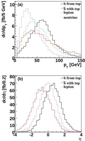
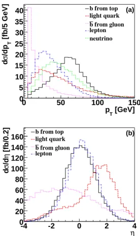
Figures 3 and 4 shows the transverse momenta and pseudorapidities η [14] for the partons in our modeling of the s-channel and t-channel single top quark processes, after decay of the top quark and W boson.
[GeV] T p 0 50 100 150 [fb/5 GeV] T /dp σ d 0 2 4 6 8 10 b from top with top b lepton neutrino (a) η -4 -2 0 2 4 [fb/0.2] η /d σ d 0 10 20 30 40 50 60 70 80 b from top with top b lepton (b)
FIG. 3: Distributions of transverse momenta (a) and pseudo-rapidity (b) for the final state partons in s-channel single top quark events. The histograms only include the final state of
t, not ¯t.
The final state fermions from the top quark decay have relatively high transverse momenta and central rapidi-ties. Since the s-channel process involves the decay of a heavy virtual object, the ¯b quark produced with the top quark is also at high transverse momentum and cen-tral pseudorapidity. By contrast, the light quark in the t-channel appears at lower transverse momentum and at more forward pseudorapidities because it is produced when an initial state parton emits a virtual W boson. The ¯b quark from t-channel initial state radiation appears typically at very low pT and with large pseudorapidities and is thus often not reconstructed experimentally.
Due to its electroweak nature, single top quark produc-tion results in a polarized final state top quark. It has
[GeV] T p 0 50 100 150 [fb/5 GeV] T /dp σ d 0 5 10 15 20 25 30 35 40 b from top light quark from gluon b lepton neutrino (a) η -4 -2 0 2 4 [fb/0.2] η /d σ d 0 20 40 60 80 100 120 140
160 b from toplight quark from gluon b
lepton
(b)
FIG. 4: Distributions of transverse momenta (a) and pseudo-rapidity (b) for the final state partons in t-channel single top quark events. The histograms only include the final state of
t, not ¯t.
been shown [15] that the top quark spin follows the direc-tion of the down-type quark momentum in the top quark rest frame. This is the direction of the initial ¯d quark for the s-channel and close to the direction of the final state d quark for the t-channel. The above result follows directly from the properties of the polarized top quark decays when single top quark production is considered as top quark decay going “backwards in time” [16].
C. Overview of the Backgrounds
Searches for single top quark production are challeng-ing because of the very large backgrounds. The situation is significantly different from top pair production not just because of the smaller production rate, but more impor-tantly because of the smaller multiplicity of final state particles (leptons or jets). Single top quark events are typically less energetic (because there is only one heavy object), less spherical (because of the production mech-anism), and typically have two or three jets, not four as do t¯t events.
Processes that can have the same single top quark
experimental signature include in order of importance W +jets, t¯t, multijet production, and some smaller con-tributions from Z+jets and diboson events.
• W +jets events form the dominant part of the back-ground. The cross section for W +2 jets produc-tion is over 1000 pb [17, 18] with W b¯b contributing about 1%.
• The second largest background is due to t¯t pro-duction. This process has a larger multiplicity of final state particles than single top quark events. However, when some of the jets or a lepton are not identified, the kinematics of the remaining particles are very similar to those of the signal.
• Multijet events form a background in the electron channel when a jet is misidentified as an electron. The probability of such misidentification is rather small, but the ≥3 jet cross section is so large that the overall contribution is significant.
Additionally, b¯b production contributes to the back-ground when one of the b’s decays semileptonically. This background in the electron channel is very small. In the muon channel, b¯b events form a back-ground when the muon is away from the jet axis or when the jet is not reconstructed.
• Z/Drell-Yan+jets production can mimic the single top quark signals if one of the leptons is misidenti-fed.
• W W , W Z, and ZZ processes are the electroweak part of the W +jets and Z+jets backgrounds, but with different kinematics.
Single top quark events are kinematically and topolog-ically similar to W +jets and t¯t events. Therefore, ex-tracting the signal from the backgrounds is challenging in a search for single top quark production.
D. Status of Searches
Both the CDF and DØ collaborations have previ-ously performed searches for single top quark produc-tion [19, 20]. Recently, CDF performed a search using 160 pb−1 of data and obtained upper limits of 13.6 pb (s-channel), 10.1 pb (t-channel), and 17.8 pb (s+t com-bined) at the 95% confidence level [21]. DØ has published a neural network search for single top quark production using 230 pb−1 of data [22], which is described in more detail in this article.
E. Outline of the Analysis
We have performed a search for the electroweak pro-duction of single top quarks in the s-channel and t-channel production modes with the DØ detector at the
Fermilab Tevatron collider. We consider lepton+jets in the final state, where the lepton is either an electron or a muon.
To take advantage of the differences between s- and t-channel final state topologies, we differentiate the s-channel search from the t-s-channel search by requiring at least one untagged jet in the t-channel search. For both s-channel and t-channel searches, we separate the data into independent analysis sets based on the lepton flavor (e or µ) and the multiplicity of identified b quarks (one tagged jet or more than one).
We use two different multivariate methods to extract the signal from the large backgrounds: a cut-based anal-ysis, first presented here, and an analysis based on neu-ral networks that was first presented in brief form in Ref. [22]. In the absence of any significant evidence for signal, we set upper limits at the 95% C.L. on the single top quark production cross sections.
Finally, we present limit contours in a two-dimensional plane of the s-channel signal cross section versus the t-channel signal cross section.
F. Outline of the Paper
This paper is organized as follows. Section II describes the DØ detector and the reconstruction of the final state objects. Section III summarizes the triggers for the data samples used in the search and Section IV describes the selection requirements. Section V explains the modeling of signals and backgrounds, and Section VI presents the numbers of events passing all selections. Section VII dis-cusses the most important variables that offer discrimina-tion between the signals and backgrounds, and provides details of the cut-based and the neural network analy-ses. Section VIII lists the systematic uncertainties in this measurement. Section IX discusses the procedure for setting limits on the signal cross section using Bayesian statistics. The limits are presented in Section X, and we summarize the results in Section XI.
II. THE DØ DETECTOR AND OBJECT
RECONSTRUCTION
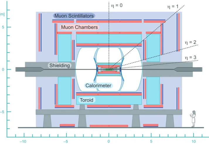
A. The DØ Detector
The DØ detector [23] is shown in Figs. 5 and 6 and consists of several layered elements. The first is a mag-netic central-tracking system, which includes a silicon mi-crostrip tracker (SMT) and a central fiber tracker (CFT), both located within a 2 T superconducting solenoidal magnet. The SMT has≈ 800, 000 individual strips, with a typical pitch of 50− 80 µm, and a design optimized for tracking and vertexing capability at pseudorapidities of |η| < 3.0. The system has a six-barrel longitudinal structure, each with a set of four layers arranged axially around the beam pipe, and interspersed with 16 radial
disks. The CFT has eight thin coaxial barrels, each sup-porting two doublets of overlapping scintillating fibers of 0.835 mm diameter, one doublet being parallel to the collision axis, and the other alternating by±3◦ relative to the axis. Light signals are transferred via clear light fibers to solid-state photon counters (visible light photon counters, VLPCs) that have≈ 80% quantum efficiency.
Central and forward preshower detectors are located just outside of the superconducting coil (in front of the calorimetry). These are constructed of several layers of extruded triangular scintillator strips that are read out using wavelength-shifting fibers and VLPCs. The next layer of detection involves three liquid-argon/uranium calorimeters: a central section (CC) covering |η| up to ≈ 1, and two end calorimeters (EC) extending coverage to |η| ≈ 4, all housed in separate cryostats [24]. In ad-dition to the preshower detectors, scintillators between the CC and EC cryostats provide sampling of developing showers for 1.1 <|η| < 1.4.
A muon system resides beyond the calorimetry, and consists of a layer of tracking detectors and scintillation trigger counters before 1.8 T iron toroids, followed by two more similar layers after the toroids. Tracking for |η| < 1 relies on 10 cm wide drift tubes [24], while 1 cm mini drift tubes are used for 1 <|η| < 2.
The luminosity is obtained from the rate of inelastic collisions measured using plastic scintillator arrays lo-cated in front of the EC cryostats, covering 2.7 <|η| < 4.4.
B. Object Reconstruction
Physics objects are reconstructed from the digital sig-nals recorded in each part of the detector. Particles can be identified by certain patterns and, when correlated with other objects in the same event, they provide the basis for understanding the physics that produced such signatures in the detector.
1. Primary Vertex
The position of the hard scatter interaction is deter-mined at DØ by clustering tracks into seed vertices using a Kalman filter algorithm [25]. The primary vertex is then selected using a probability function based on the pT values of the tracks assigned to each vertex. The hard scatter vertex is distinguished from other soft interaction vertices by the higher average pT of its tracks. In multijet data events, the position resolution of the primary ver-tex in the transverse plane (perpendicular to the beam pipe) is around 40 µm, convoluted with a typical beam spot size of around 30 µm. For the longitudinal direction (along the beam pipe), the typical resolution is about 1 cm.
Calorimeter
Shielding
Toroid
Muon Chambers
Muon Scintillators
η = 0
η = 1
η = 2
[m]η = 3
–10 –5 0 5 10 –5 0 5FIG. 5: General view of the DØ detector. The proton beam travels from left to right and the antiproton beam from right to left in this figure.
2. Electrons
Electron candidates are initially identified as energy clusters in the central region of the electromagnetic calorimeter,|η| ≤ 1.1. We define two classes of electron candidates: loose and tight. Loose electrons are required to have the fraction of their total energy deposited in the electromagnetic (EM) calorimeter fEM > 0.9 and a shower-shape chi-squared, based on seven variables that compare the values of the energy deposited in each layer of the electromagnetic calorimeter with average distri-butions from simulated electrons, to be χ2
cal < 75. Fi-nally, loose electron candidates are also required to be isolated by measuring the total deposited energy and the energy from the EM calorimeter only around the electron track: ETotal(R < 0.4) < 1.15× EEM(R < 0.2), where R =p(∆φ)2+ (∆η)2 is the radius of a cone defined by the azimuthal angle φ and the pseudorapidty η.
For an electron candidate to be included in the tight class, a track must be matched to the loose cluster within |∆η| < 0.05 and |∆φ| < 0.05, and additionally pass a cut on a seven-variable likelihood built to separate real electrons from backgrounds. The following variables are used in the likelihood: (i) fEM; (ii) χ2cal; (iii) ETcal/ptrackT , transverse energy of the cluster divided by the transverse
momentum of the matched track; (iv) χ2 probability of the track match; (v) distance of closest approach between the track and the primary vertex in the transverse plane; (vi) Ntracks, the number of tracks inside a cone of R < 0.05 around the matched track; and (vii)P pT of tracks in an R < 0.4 cone around the matched track. Tight electrons are obtained by applying a cut on the likelihood of L > 0.85. The overall tight electron identification efficiency in data is around 75%.
A comparison between the dielectron invariant mass distributions for Z→ ee simulated events and data shows that the position of the simulated Z boson peak is shifted from that in data, and that the electron energy resolution is better than in data. We apply small corrections to the identification efficiency and electromagnetic energy of simulated electrons and smear their energies to agree with data.
3. Muons
Muons are reconstructed in DØ up to |η| = 2 by first finding hits in all three layers of the muon spectrometers and requiring that the timing of these hits is consistent with the hard scatter, thus rejecting cosmic rays.
Sec-Solenoid Preshower Fiber Tracker Silicon Tracker η = 0 η = 1 η = 2 [m] η = 3 –0.5 0.0 –1.5 –1.0 0.5 1.0 1.5 –0.5 0.0 0.5
FIG. 6: Close view of the tracking systems.
ondly, all muon candidates must be matched to a track in the central tracker. That central track must pass the following criteria: (i) chi-squared per degree of freedom less than 4; (ii) the distance of closest approach to the primary vertex in the transverse plane must be less than three standard deviations; and (iii) the distance in z be-tween the track and the primary vertex must be less than 1 cm.
As for electrons, we similarly define two classes: loose and tight, but this time based solely on the muon’s iso-lation from other objects. A loose isolated muon must comply with R(muon, jet) > 0.5, which is the distance between the muon and the jet axis. A tight isolated muon must be loose and additionally satisfy track-based and calorimeter-based criteria: |Ptracksp
T/pT(µ)| < 0.06 where the sum is over tracks within a cone of R(track, muon)< 0.5; and |PcellsE
T/pT(µ)| < 0.08 where the sum is over calorimeter cells within an anulus of 0.1 < R(calorimeter cell, muon)< 0.4. The overall tight muon identification efficiency in data is around 65%.
Similarly to electrons in the simulation, we correct the energy scale for simulated muons and smear their energies to reproduce the data in Z→ µµ.
4. Jets
We reconstruct jets based on calorimeter cell energies, using the improved legacy cone algorithm [26] with radius
R = 0.5. Noisy calorimeter cells are ignored in the re-construction algorithm by imposing the requirement that neighboring cells have signals above the noise level.
Jet identification is based on a set of cuts to reject poor quality jets or noisy jets: (i) 0.05 < fEM < 0.95; (ii) fraction of jet ET in the coarse hadronic calorimeter layers < 0.4; (iii) ratio of ET’s of the most energetic cell to the second most energetic cell in the jet < 10; and (iv) smallest number of towers that make up 90% of the jet ET, n90> 1.
Jet energy scale corrections are applied to convert jet energies from the reconstructed level into particle-level energies. The reconstructed fully-corrected energy of jets from the simulation of the detector performance does not exactly match that seen in data. Similar to electrons and muons, we smear jet energies by a small amount in the simulation to reproduce the resolution measured in data.
5. Missing Energy
We infer the transverse energy of the neutrino in the event as the opposite of the vector sum of all the energy deposited in the calorimeter. This calorimeter-only miss-ing transverse energy is then corrected with the jet energy scale, the electromagnetic scale, and the energy loss from isolated muons in the calorimeter and their momenta.
C. Identification of b-Quark Jets
The presence of b quarks can be inferred from the long lifetime of B hadrons, which typically travel a few mil-limeters before hadronization. Thus b-quark jets contain a displaced vertex inside a jet whereas light-quark jets do not. The Secondary Vertex Tagger (SVT), described below, makes use of this fact to identify, or tag, b-quark jets by fitting tracks in the jet into a secondary vertex.
1. Taggability
Before the b-quark tagging algorithm is applied to iden-tify displaced vertices in the jet, a set of cuts is applied to ensure a good quality jet and factor out detector ge-ometry effects. Thus the final probability to identify a b-quark jet is factored into two parts: a taggability part, or jet-quality-sensitive component, and a tagger part, or heavy-flavor-sensitive component. A taggable jet re-quires at least two tracks within a cone of R = 0.5. At least one of these tracks must have pT > 1.0 GeV, and additional tracks must have pT > 0.5 GeV. All tracks must have at least one SMT hit, an xy distance-of-closest-approach (DCA) of < 0.2 cm, and a z DCA of < 0.4 cm with respect to the primary vertex. The taggability is the number of taggable jets divided by the number of good jets. Only jets satisfying jet identification require-ments, with pT > 15 GeV (after jet energy corrections) and|η| ≤ 2.5 are considered to be good for the definition of taggability.
In simulated events, the taggability is higher than in data mainly due to a non-comprehensive description of the tracking detectors (dead detector elements, other in-efficiencies, noise, etc.) resulting in a higher tracking ef-ficiency (in particular within jets). Therefore, the Monte Carlo taggability must be calibrated to that observed in the data. A taggability-rate function is utilized to do this by parametrizing the taggability as a function of jet pT and η. Thus, the taggability per jet is determined in data and applied to the Monte Carlo as:
Ptaggable(p T, η) =
# taggable jets in (pT, η) bin # jets in (pT, η) bin
. (1) Central jets with momenta above 40 GeV have taggabil-ities of around 85%. For simulated jets the taggability is ≈ 90%.
2. Secondary Vertex Tagger
The SVT algorithm is designed to reconstruct a dis-placed vertex inside a jet by fitting tracks that have a large impact parameter from the hard scatter ver-tex. A simple algorithm is applied to the tracks to re-move most K0
S’s, Λ’s, and photon conversions. Tracks are then required to have at least two SMT hits,
pT > 1.0 GeV, transverse impact parameter significance (dca/σdca) greater than 3.5, and a track χ
2> 10. A sim-ple cone jet-algorithm is used to cluster the tracks into track-jets, and then a Kalman filter algorithm is used to find vertices with the tracks in each track-jet. The distance between the primary vertex and the found sec-ondary vertex, the decay length Lxy, and its error σLxy
are calculated taking into account the uncertainty on the primary vertex position. The decay length is a signed parameter, defined by the sign of the cosine of the angle between the vector from the primary vertex to the decay point and the total momentum of the tracks attached to the secondary vertex. If the decay length significance Lxy/σLxy is more than 7, then the found vertex is
con-sidered a tag. A calorimeter jet is concon-sidered tagged if the distance between the jet axis and the line joining the primary vertex and the secondary vertex is R < 0.5 in η, φ space. This set of cuts has been tuned to obtain a probability for a light quark mistag of 0.25%. Note that gluon jets are included in the light quark category.
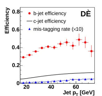
We estimate the b tagging efficiency in a dijet data sample. The heavy flavor content of the sample is en-hanced by requiring one of the jets to have a high-pT muon relative to the jet axis. The SVT efficiency to tag the other jet can then be inferred. We estimate the c quark tagging efficiency from a Monte Carlo simulation. The mis-tagging rate, or how often a light-flavor jet (from u, d, s quarks or gluons) is identified as a b jet, is also measured in a dijet data sample. We count the num-ber of found secondary vertices with Lxy/σLxy <−7 and
correct for the contribution of heavy-flavor jets in the sample and the presence of long-lived particles in light-flavor jets. The sign in the decay length measurement comes from the scalar product of the decay length vector and the unit vector defined by the Figure 7 shows the tagging efficiency as a function of jet pT for the different types of jets.
To calculate the probability for a simulated jet to be tagged, a tag-rate function (TRF) derived from data is used similarly to the taggability parametrized in pT and η:
Ptagging(pT, η) =
# SVT tagged jets in (pT, η) bin # taggable jets in (pT, η) bin
. (2) Separate functions are determined for b-quark jets, c-quark jets, and light-c-quark jets, as in Fig. 7.
The TRFs are applied to the Monte Carlo samples in the following way. First, for each jet in the event (with pT > 15 GeV and |η| < 3.4) a taggability-rate function is applied. Next, each jet’s lineage is determined. If the jet contains a B meson within R < 0.5 of the jet axis it is labeled a b-quark jet. If a D meson is within R < 0.5 of the jet axis, it is labeled a c-quark jet. If no B or D meson is found in the jet, the jet is labeled a light-quark jet. The probability determined from the appropriate TRF is then applied. The taggability and tagging probability are multiplied together to determine the probability of the simulated jet to be tagged.
[GeV]
TJet p
20
40
60
Efficiency
0
0.2
0.4
0.6
0.8
b-jet efficiency
DØ
c-jet efficiency
10)
×
mis-tagging rate (
FIG. 7: Measured b-tagging efficiency (circles) and
mis-tagging rate (triangles), and estimated c-mis-tagging efficiency
(solid line) as a function of jet pT.
In data we apply the secondary vertex algorithm di-rectly and can identify which jet is tagged and which is not. The situation in simulated events is different; the TRFs return a probability (or weight) rather than a tagged/not-tagged answer per jet. Since many of the discriminant variables used later on in the analysis (see Sec. VII A) need to know which jet was tagged, each pos-sible combination of tagged and untagged jets is consid-ered for every simulated event. Thus each event is used repeatedly in the analysis, considering each time a differ-ent jet as tagged. The probability of each combination is calculated using the tag rate functions, and combined with the overall event weight. The sum of the weights for all the possible combinations of each event is equal to the original probability for an event to have at least one tagged jet.
The use of all permissible tagged jet combinations in each simulated event is a very powerful tool. It ensures that the kinematic distributions in histograms of tagged events have the correct shape, and it allows tagged jet in-formation to be used in variables for signal/background separation, since the final classifiers are trained with weighted events.
III. TRIGGERS AND DATA SET
The DØ trigger system is composed of three levels. The first level consists of hardware and firmware com-ponents, the second level uses information from the first level to construct simple physics objects, and the third level is software based and performs full event reconstruc-tion.
The DØ calorimeter is used to trigger events based on the energy deposited in towers of size ∆η×∆φ = 0.2×0.2
that are segmented longitudinally into electromagnetic and hadronic sections. The level 1 electron trigger re-quires electrons to be above a certain threshold: ET ≡ E sin θ > T where E is the energy deposited in the tower, θ is the angle between the beam and the trigger tower from the center of the detector, and T is the programmed threshold. The level 2 electron trigger uses a seed-based clustering algorithm that sums the energy deposited in two neighboring towers and has the ability to make a decision based on the threshold of the cluster, the elec-tromagnetic fraction, and isolation of the electron. The level 3 electron trigger uses a simple cone algorithm with R < 0.25 and requirements on the ET, the electromag-netic fraction, and the quality of the transverse shower shape.
The level 1 jet trigger is similar to the electron trigger tower algorithm, but includes the energy deposited in the hadronic portion of the calorimeter. The level 2 jet trig-ger uses a seed-based clustering algorithm summing the energy deposition in a 5× 5 tower array. The level 3 jet algorithm is similar to the level 3 electron algorithm, but does not include a requirement on the electromagnetic fraction or shower shape.
The level 1 muon trigger examines hits from the muon wire chambers, muon scintillation counters, and tracks from the level 1 track trigger for patterns consistent with those coming from a muon. The level 2 muon trigger reconstructs muon tracks from both wire and scintillator elements in the muon system. It can impose requirements on the number of muons, the pT and η of the muons, and the overall quality of the muons. The level 3 muon trigger uses wire and scintillator hits to reconstruct tracks using segments inside and outside the toroid.
The output of the first level of the trigger is used to limit the rate for accepted events to≈ 1.5 kHz. At the next trigger stage, with more refined information, the rate is reduced further to ≈ 800 Hz. The third level of the trigger, with access to all the event information, reduces the output rate to≈ 50 Hz, which is written to tape.
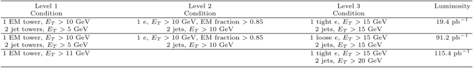
The data were acquired in the period between August 2002 and March 2004. Tables II and III show the trig-gers used to collect the data for the electron plus jets (e+jets) and muon plus jets (µ+jets) triggers and give the integrated luminosity for each trigger.
IV. EVENT SELECTION
Event selection begins after all corrections have been applied to the data. These corrections include the jet energy and the EM energy calibrations. The primary vertex, zvertex, for the event must be within the tracking fiducial region,|zvertex| < 60 cm, which allows for a suf-ficient number of tracks, Ntracks ≥ 3, associated with it to be properly reconstructed.
As discussed in Sec. I C, the single top quark signature is characterized by one isolated high-pT charged lepton,
TABLE II: Trigger conditions at levels 1, 2, and 3 for the electron plus jets trigger.
Level 1 Level 2 Level 3 Luminosity
Condition Condition Condition
1 EM tower, ET >10 GeV 1 e, ET>10 GeV, EM fraction > 0.85 1 tight e, ET >15 GeV 19.4 pb−1 2 jet towers, ET >5 GeV 2 jets, ET >10 GeV 2 jets, ET>15 GeV
1 EM tower, ET >10 GeV 1 e, ET>10 GeV, EM fraction > 0.85 1 loose e, ET >15 GeV 91.2 pb−1 2 jet towers, ET >5 GeV 2 jets, ET >10 GeV 2 jets, ET>15 GeV
1 EM tower, ET >11 GeV 1 tight e, ET >15 GeV 115.4 pb−1
2 jets, ET>20 GeV
TABLE III: Trigger conditions at levels 1, 2, and 3 for the muon plus jets trigger.
Level 1 Level 2 Level 3 Luminosity
Condition Condition Condition
1 µ, | η |< 2.0 1 µ, | η |< 2.0 1 jet, ET>20 GeV 113.7 pb−1
1 jet tower, ET >5 GeV
1 µ, | η |< 2.0 1 µ, | η |< 2.0 1 jet, ET>25 GeV 113.7 pb−1
1 jet tower, ET >3 GeV 1 jet, ET >10 GeV
6ET, and two to four jets. We accept events with three or four jets in order to include contributions from extra gluons and quarks. The b jet from the single top quark decay tends to be more energetic than the other jets as-sociated with the event, so we require a higher ET for the leading jet. Table IV lists the requirements of the initial selection.
TABLE IV: Initial event selection requirements.
Selection Cut e+jets µ+jets
tight e, ET≥ 15 GeV =1 =0 tight µ, ET ≥ 15 GeV =0 =1 6ET ≥ 15 GeV Njets 2 ≤ Njets≤ 4 ET(jet) ≥ 15 GeV |η(jet)| ≤ 3.2 ET(jet1) ≥ 25 GeV |η(jet1)| ≤ 2.4
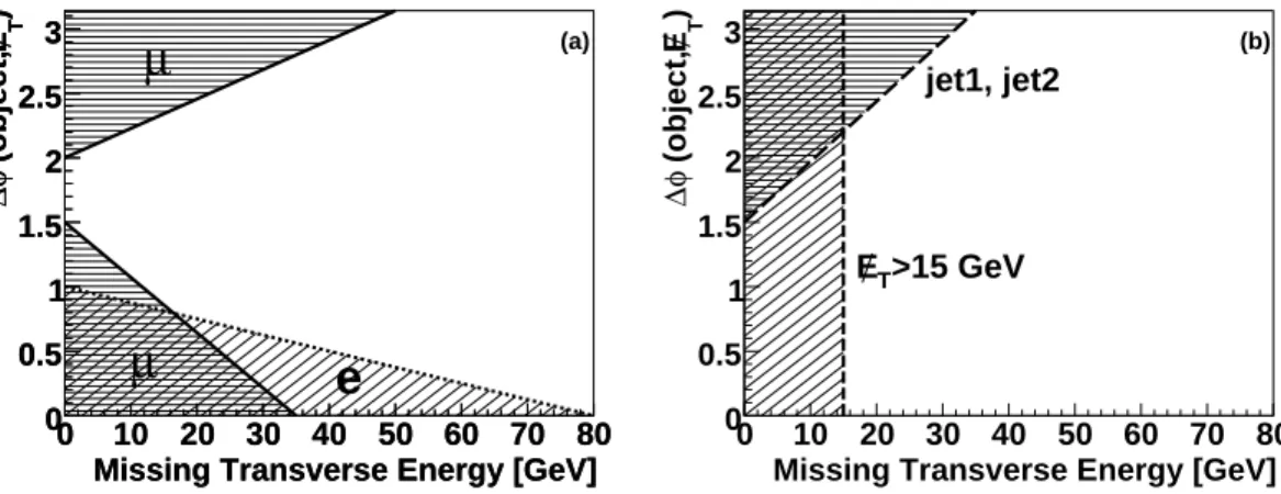
In addition, we make a set of cuts that remove misre-constructed events, also known as “triangle cuts.” If the transverse energy of an object is mismeasured, this tends to create false missing energy in a parallel or antiparallel direction. The triangle cuts remove these mismeasured events, which are difficult to model, but do not affect the signal appreciably because there is very small signal ac-ceptance in these kinematic regions. In Fig. 8, we show the kinematic regions that are removed by the triangle cuts.
From the selected jets in the event, at least one b-tagged jet must be found. For the t-channel analysis, at least one jet must be untagged. This requirement comes from the fact that one of the main features of the t-channel signal is that a light-quark jet exists in the final state. The events are then divided into subsets consisting of the number of tagged jets found in the event:
single-tagged or double-single-tagged. Since the t-channel requires at least one untagged jet, there are no two-jet events in the double-tagged sample in the double-tagged t-channel search.
V. SIGNAL AND BACKGROUND MODELING
In order to compare the observed event yield in data with our expectation, and to set limits on the single top quark production cross sections, we determine ac-ceptances and event yields for the single top quark sig-nals and the various SM background contributions. This estimation is based primarily on simulated samples for shapes of distributions, except for the multijet back-ground where we use data samples. The yield normal-ization is based on theoretical cross sections, except for the W +jets and multijet backgrounds which are normal-ized to data.
A. Acceptance and Yield for Simulated Samples
The acceptance α for a particular simulated signal or background sample is calculated as:
α = 1
NMC X
i
wi (3)
where the sum is over simulated events that pass the selection cuts and is normalized to the total number of simulated events in the sample NMC. The event weight wi is given by: wi = ǫlepton IDi × ǫ jet ID i × ǫ trigger i × ǫ btagging i (4)
and includes correction factors ǫ to account for effects not modeled and for cuts not applied to the simulated
Missing Transverse Energy [GeV] 0 10 20 30 40 50 60 70 80 ) T E (object, φ∆ 0 0.5 1 1.5 2 2.5 3
Missing Transverse Energy [GeV]
0 10 20 30 40 50 60 70 80 ) T E (object, φ∆ 0 0.5 1 1.5 2 2.5 3
µ
µ
e
(a)Missing Transverse Energy [GeV]
0 10 20 30 40 50 60 70 80 ) T E (object, φ∆ 0 0.5 1 1.5 2 2.5 3 jet1, jet2 >15 GeV T E (b)
FIG. 8: Kinematic regions excluded in the e+jets and µ+jets analyses by the triangle cuts applied in the (∆φ(object, 6ET), 6ET)
plane, where each object can be: the tight isolated electron or muon (a), and the leading and second leading jets (b). The shaded areas are excluded.
samples. Trigger requirements are not made in the simu-lation (see Sec. III) and the correction factors ǫtriggeri are about 90%. Furthermore, we do not require b tagging in simulated events, and the correction factor ǫbitagging averages about 55% for s-channel events and about 40% for t-channel events.
The yield estimate Y is given by the product of ac-ceptance, integrated luminosity L, theory cross section σtheory, and branching fraction B:
Y = α × L × σtheory
× B. (5)
The branching fraction factor gives the fraction of events that result in the final state lepton of interest (e or µ). The yield includes a small contribution from W → τ decays where the τ decays to e or µ.
B. Single Top Quark Signals
The Comphep matrix element generator [27] has been used to model single top quark s-channel and t-channel signal events. We include not only the leading order Feynman diagrams in the event generation, but also the O(αs) diagrams with real gluon radiation in order to reproduce NLO distributions. For the t-channel sam-ple, we include both the leading order diagram (Fig. 2 (a)) and the W -gluon fusion diagram (Fig. 2 (b)) explic-itly, generating W -gluon fusion events for the region of phase space where the ¯b quark from gluon splitting has pT(¯b) > 17 GeV and leading order events otherwise.
C. t¯t Background
Top quark pair production contributes as a background both in the lepton+jets and in the dilepton decay chan-nels. This background is modeled using alpgen [17], and the yields are normalized to the theory cross section (see Sec. I C).
D. W W and W Z Backgrounds
The backgrounds from diboson production are mod-eled using alpgen, and the yields are normalized to the theory cross sections [28].
E. Multijet and W +jets Backgrounds
The backgrounds from multijet (fake lepton) and W +jets production are normalized to the data sample before b tagging [29]. We start from a data sample pass-ing all selection cuts includpass-ing the loose lepton require-ments (see Sec. II B). From that sample, we select a sub-set of events that also pass the tight lepton requirements. In addition, we determine the probabilities for real and fake leptons to pass the tight lepton requirement. These two probabilities together with the numbers of events in the two samples then allow us to calculate the number of real and fake lepton events in the W +jets and multijet background samples [30].
The shapes of the distributions for the multijet back-ground are modeled using a data sample that passes all selection cuts but fails the tight lepton identification re-quirements. The shapes of distributions for the W +jets background are modeled using alpgen W +2jets events.
1. Multijet Background
A part of the background comes from events in which jets are misidentified as isolated leptons. In the electron channel, this background is typically produced by jets that contain a π0, which, together with a randomly asso-ciated track, is misreconstructed as an isolated electron since it decays to two photons. In the muon channel, this background is typically produced by heavy-flavor jets in which a muon from a semileptonic decay is
misrecon-structed as an isolated high-pT muon.
The multijet background is estimated purely from data. We use multijet data samples that pass all event selection requirements, but fail the requirement on tight muon isolation or tight electron quality (see Sec. II B) to determine the kinematic shape of distributions. These samples are normalized to the multijet background esti-mate in the data sample after event selection, but before requiring a b tag.
2. W+Jets Background
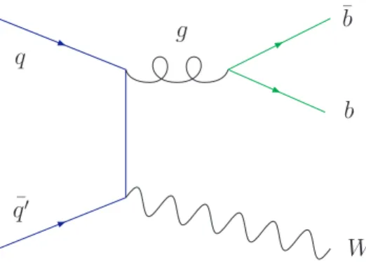
An example Feynman diagram for W +2 jet production is shown in Fig. 9. This background is modeled from a simulated W jj sample (j = u, d, s, c, g), which includes not just light-quark flavors but also c quarks (considered massless in this model). We use a separate sample for W b¯b and explicitly exclude events with b quarks from the W jj sample. The parton level samples were generated with alpgen.
q
¯
q
′¯b
b
W
g
FIG. 9: Representative Feynman diagram for W b¯b produc-tion.
Since the W +jets background is normalized to data (after subtraction of the small t¯t and diboson content), it includes all sources of W +jets events with a similar flavor composition, in particular Z+jets events where one of the leptons from the Z boson decay is not identified.
F. Detector Simulation
The parton-level samples for the single top quark sig-nals, t¯t, W +jets, W W , and W Z backgrounds are pro-cessed with pythia [31] for hadronization and modeling of the underlying event, using the cteq5l [32] parton dis-tribution functions. tauola [33] is used for tau lepton decays and evtgen [34] for B hadron decays. The gen-erated events are processed through a geant-based [35] simulation of the DØ detector.
VI. EVENT YIELDS
The expected event yields for the various background contributions are calculated from both simulated samples and data. The expected event yield for the single top quark signal is calculated from simulated samples and normalized to the theoretical cross sections.
The total background event yieldY is given by the sum over all backgrounds:
Y =X
i
Yi (6)
where each individual yieldYi is given by Eq. 5 for the various MC samples.
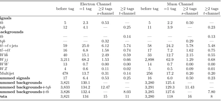
Table V shows the numbers of events for each of the signals, combinations of signals, backgrounds, and data, after event selection and b tagging. The background sum reproduces the data within uncertainties for all samples after b tagging.
A summary of the yield estimates for the signal and backgrounds and the numbers of observed events in data after selection, including the systematic uncertainties as described in Sec. VIII, is shown in Table VI.
After b tagging, the W +jets background makes up around 60% of the total background model (48% W jj, 12% W b¯b), the t¯t background is around 27% (21% lep-ton+jets, 6% dilepton), 10% is mainly multijet back-ground, and s-channel single top quark production pro-vides 3% in the t-channel search and vice versa.
VII. EVENT ANALYSIS
Table V shows that even after event selection and b tag-ging, the expected single top quark signal yield is small compared to the overwhelming backgrounds. Additional steps are necessary in order to separate the signal and background. In this section, we first present kinematic variables that allow us to separate the s-channel or t-channel single top quark signal from the backgrounds. We then describe a cut-based analysis and a neural net-works analysis that use these variables.
A. Discriminating Variables
In this section we introduce the variables that we found to be most effective in separating the single top quark signals from the backgrounds. The list of discriminating variables has been chosen based on an analysis of Feyn-man diagrams of signals and backgrounds [36] and on a study of single top quark production at NLO [11, 12].
The variables fall into three categories: individual ob-ject kinematics, global event kinematics, and variables based on angular correlations. The list of variables is shown in Table VII.
TABLE V: Event yields after selection in the electron and muon channels.
Electron Channel Muon Channel
before tag =1 tag ≥2 tags ≥2 tags before tag =1 tag ≥2 tags ≥2 tags
s-channel t-channel s-channel t-channel
Signals tb 5 2.3 0.53 — 5 2.2 0.50 — tqb 12 4.1 — 0.25 11 3.9 — 0.23 Backgrounds tb — — — 0.14 — — — 0.13 tqb — — 0.32 — — — 0.29 — t¯t→ℓ+jets 59 25.0 6.12 5.74 58 24.2 5.78 5.48 t¯t→ℓℓ 16 6.8 1.58 0.74 17 7.2 1.62 0.75 W b¯b 40 15.1 2.49 0.59 33 12.7 2.15 0.55 W jj 3,211 68.2 1.53 0.66 2,898 62.9 1.29 0.68 W W 13 0.7 0.00 0.00 14 0.7 0.00 0.00 W Z 4 0.6 0.11 0.02 5 0.5 0.09 0.01 Multijet 478 13.7 0.31 0.14 256 17.2 0.20 0.20 Summed signals 17 6.4 0.53 0.25 16 6.0 0.50 0.23 Summed backgrounds 3,821 130.1 — — 3,280 125.4 — — Summed backgrounds+tqb 3,833 134.2 12.47 — 3,291 129.3 11.43 — Summed backgrounds+tb 3,826 132.4 — 8.03 3,285 127.6 — 7.80 Data 3,821 134 15 11 3,280 118 16 8
TABLE VI: Estimates for signal and background yields and the numbers of observed events in data after event selection for the electron and muon, single-tagged and double-tagged analysis sets combined. The W +jets yields include the di-boson backgrounds. The total background for the s-channel (t-channel) search includes the tqb (tb) yield. The quoted yield uncertainties include systematic uncertainties taking into ac-count correlations between the different analysis channels and samples.
Source s-channel search t-channel search
tb 5.5 ± 1.2 4.8 ± 1.0 tqb 8.6 ± 1.9 8.5 ± 1.9 W+jets 169.1 ± 19.2 163.9 ± 17.8 t¯t 78.3 ± 17.6 75.9 ± 17.0 Multijet 31.4 ± 3.3 31.3 ± 3.2 Total background 287.4 ± 31.4 275.8 ± 31.5 Observed events 283 271
In order to get optimum separation between signal and background, the single top quark final state is re-constructed according to whether a variable is primarily used in the s-channel or the t-channel search. The W bo-son from the top quark decay is reconstructed from the isolated lepton and the missing transverse energy. The z-component of the neutrino momentum is calculated using a W boson mass constraint, choosing the solution with smaller|pν
z| from the two possible solutions. The candi-date top quark is reconstructed from this W boson and a jet. This jet is chosen to be either the leading b-tagged jet or the best jet. In the t-channel analysis, there is typically only one high-pT b quark jet in the final state,
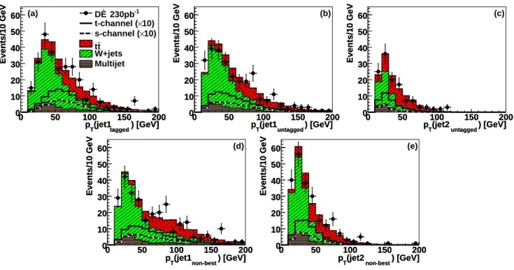
thus the leading b-tagged jet is chosen to reconstruct the top quark. By contrast, in the s-channel there are two high-pT b quark jets in the final state, and a choice needs to be made between them. Furthermore, typically only one of the two is identified as a b-tagged jet. We use the best-jet algorithm [19] to identify this jet without using b tagging information. The best jet is defined as the jet in each event which gives, together with the reconstructed W boson, an invariant mass closest to 175 GeV. Jets that have not been identified by the b tagging algorithm are called “untagged” jets.
Figures 10 to 14 show all discriminating variables used in this analysis, comparing the single top quark signal dis-tributions to those of the background sum and the data. Good agreement between the data and the background model is seen in all cases.
B. Cut-Based Analysis
This analysis takes the discriminating variables, chooses the best subsets, and finds the optimal points to cut on them in order to improve the expected cross section limits by increasing the signal to background ra-tio.
Optimization of the cut positions is performed by us-ing the signal Monte Carlo events to seed the cut values scanned in the algorithm. The signal and background pass rates are determined for each cut point, an expected limit on the cross section is obtained from these, and the best result is used as the operating point of the analysis. The strategy is to look at the s- and t-channel pro-cesses separately to take full advantage of the