Distributed algorithms for dynamic topology construction and their applications

Distributed Algorithms for

Dynamic Topology Construction and Their Applications

by

Ching Law

M.Eng., Electrical Engineering and Computer Science

MIT, 1999

S.B., Computer Science and Engineering

MIT, 1998

S.B., Mathematics

MIT, 1998

Submitted to the

Department of Electrical Engineering and Computer Science

in partial fulfillment of the requirements for the degree of

Doctor of Philosophy

at the

MASSACHUSETTS INSTITUTE OF TECHNOLOGY

September 2004

©

Massachusetts Institute of Technology 2004. All rights reserved.

Author ...

Department of Electrical Engineering and Computer Science

August 31, 2004

Certified by...

...

Kai-Yeung Siu

Associate Professor

Thesis Supervisor

OF

Arthur C. Smith

Distributed Algorithms for Dynamic Topology Construction and Their Applications

by

Ching Law

Submitted to the Department of Electrical Engineering and Computer Science on August 31, 2004, in partial fulfillment of the

requirements for the degree of Doctor of Philosophy

Abstract

We introduce new distributed algorithms that dynamically construct network topologies. These algorithms not only adapt to dynamic topologies where nodes join and leave, but also actively set up and remove links between the nodes, to achieve certain global graph properties.

First, we present a novel distributed algorithm for constructing overlay networks that are composed of d Hamilton cycles. The protocol is decentralized as no globally-known server is required. With high probability, the constructed topologies are expanders with O(logd n) diameters and 2v'2d- 1+ e second largest eigenvalues. Our protocol exploits the properties of random walks on expanders. A new node can join the network in O(logdn) time with 0(d logd n) messages. A node can leave in 0(1) time with 0(d) messages.

Second, we investigate a layered construction of the random expander networks that can implement a distributed hash table. Layered expanders can achieve degree-optimal routing at O(logn/loglogn) time, where each node has O(logn) neighbors. We also analyze a self-balancing scheme for the layered networks.

Third, we study the resource discovery problem, in which a network of machines discover one another by making network connections. We present two randomized algorithms to solve the resource discovery problem in 0(logn) time.

Fourth, we apply the insight gained from the resource discovery algorithms on general networks to ad hoc wireless networks. A Bluetooth ad hoc network can be formed by inter-connecting piconets into scatternets. We present and analyze a new randomized distributed protocol for Bluetooth scatternet formation. We prove that our protocol achieves 0(logn) time complexity and 0(n) message complexity. In the scatternets formed by our protocol, the number of piconets is close to optimal, and any device is a member of at most two piconets.

Thesis Supervisor: Kai-Yeung Siu Title: Associate Professor

Acknowledgments

First, I must thank my adviser Professor Kai-Yeung (Sunny) Siu for encouraging and sup-porting me throughout my graduate school career. Sunny has provided me enviable freedom in choosing my research directions.

A substantial portion of this thesis appeared in papers I coauthored with Sunny. Chap-ter 5 is based on papers I coauthored with Amar Mehta and Sunny.

I should also thank my thesis committee members Professor Piotr Indyk and Professor David Karger, for reading my thesis and offering invaluable suggestions to improve it.

I thank Professor Charles Leiserson. It was Charles' 6.046 take-home exam that gave me the first glimpse into computer science research. Charles accepted me as an undergraduate researcher, supervised my Master's thesis, and continued to guide me whenever I went to him for advice.

I would like to thank Professor Sanjay Sarma for the generous research assistantship support I received from the Auto-ID Center. I thank Professor Albert Meyer and Dr. Eric Lehman for taking me as his teaching assistant for 6.042. I am also grateful to my supervisor Dr. Ashwini Nanda at IBM Watson Research Center for two rewarding summer internships. Kayi Lee has been my best companion in our studies in Computer Science at MIT. Discussing algorithms with him has always been enjoyable. He has given me much help with this thesis.

I have benefited from the knowledge and wisdom of other members in Sunny's research group. In particular, I would like to thank Anthony Kam and Paolo Narvaez.

I also want to thank my friends who have read my thesis or offered suggestions for its defense presentation-Henry Lam, Kayi Lee, Philip Lee, Alan Leung, Ting Li, and Joyce Ng.

I thank my sister Cindy for listening to my ramblings. Two critical ideas in this thesis originated from our discussions during our trips in China. Last but not least, I want to thank my parents for their support and patience through all these years.

Contents

1 Introduction

1.1 Motivations . . . ..

1.1.1 Special Interest Networks . . . .. 1.1.2 Distinctions . . . .. 1.2 Theoretical Results . . . .. 1.2.1 Random Expander Networks . . . .. 1.2.2 Layered Expander Networks . . . .. 1.2.3 Resource Discovery and Connectivity . . . 1.2.4 Algorithms on Dynamic Network Topology 1.3 Applications . . . .. 1.3.1 Distributed Lookup Service . . . .. 1.3.2 On-line Communities . . . .. 1.3.3 Bluetooth Topology Construction . . . . .. 1.4 Structure of Thesis . . . .. 2 Construction of Expander Networks

2.1 Introduction . . . .. 2.2 Preliminaries . . . .. 2.2.1 Network Model . . . .. 2.2.2 Goals and Requirements . . . .. 2.2.3 A Random Graph Approach . . . .. 2.2.4 Global Variable Server . . . .. 2.3 Construction . . . .. 2.4 Perfect Sampling . . . .. 2.4.1 Global Server . . . .. 2.4.2 Broadcast . . . .. 2.4.3 Converge-Cast . . . .. 2.4.4 Coupling From The Past . . . .. 2.5 Approximate Sampling . . . ..

. . . . . . . . . . . .

CONTENTS 2.5.1 Nodes Joining ... 34 2.5.2 Nodes Leaving ... 39 2.6 Simulation Results ... 43 2.7 Auxillary Algorithms ... 44 2.7.1 Sm all Graphs . . . . 44 2.7.2 Regeneration ... . 47 2.8 Broadcasts ... ... ... ... ... 48

2.8.1 Broadcast with a Spanning Tree . . . . 48

2.8.2 Broadcast along a Cycle . . . . 51

2.9 Searches . . . . 52

2.9.1 Search by Cycle Walk . . . . 54

2.9.2 Search by Tree Walk . . . . 55

2.9.3 Search by Random Walk . . . . 56

2.10 Network Size Estimation . . . . 57

2.10.1 Size Estimation by Mobile Agents ... ... 59

2.10.2 Cycle W alks ... 59

2.10.3 Random Walks ... 60

2.11 On-line Fault Tolerance ... . 66

2.12 Related W ork . . . . 71

2.13 Concluding Remarks . . . . 72

3 Layered Expander Networks 75 3.1 Layered H-Graphs . . . . 75

3.2 Transitions Between Complete Graphs and H-Graphs ... 80

3.3 Better Recursive Searches ... 81

3.3.1 Search with Broadcasts ... . 81

3.3.2 Search with Layered Broadcasts ... ... 84

3.4 Balancing of Layered H-Graphs ... . 94

3.4.1 Random Identifiers ... 94

3.4.2 Sampling Identifiers ... ... 97

3.5 Related W ork ... . 103

4 Resource Discovery and Connectivity 105 4.1 Introduction . . . . 105

4.2 Resource Discovery . . . . 106

4.3 The ABSORPTION Algorithm . . . . 107

4.4 Variants of ABSORPTION ... ... ... 113

4.4.1 Optimizing Pointers ... 113

4.4.2 Optimizing Messages ... 113

CONTENTS

4.5 The ASSIMILATION Algorithm ... 116

4.6 Concluding Remarks ... ... 119

5 Bluetooth Scatternet Formation 121 5.1 Introduction. ... 121

5.2 Related W ork ... 123

5.3 Preliminaries ... ... 124

5.4 Scatternet Formation ... 126

5.4.1 Algorithm . . . . 126

5.5 Performance and Properties . . . .. 135

5.5.1 Theoretical Results . . . . 135 5.5.2 Simulation Results . . . . 140 5.6 Device Discovery . . . . 142 5.6.1 Protocol . . . . 144 5.6.2 Simulation Results . . . . 144 5.7 Overall Performance . . . . 147

5.8 Variations and Extensions . . . . 148

5.8.1 Inquiry Collisions . . . . 148

5.8.2 Asynchronous Protocol . . . . 148

5.8.3 Out of Range Devices . . . 149

5.8.4 Joins, Leaves, and Faults . . . . 150

5.9 Concluding Remarks . . . . 151

List of Figures

2.1 An H-graph consisting of 3 Hamilton cycles. . . . . 22

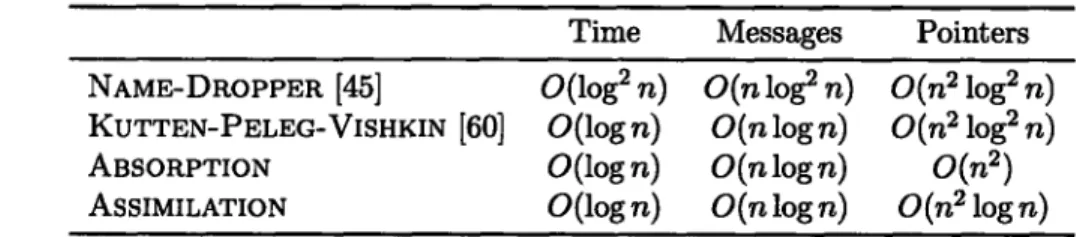
2.2 The minimum expected number of reply messages received in SAMPLE-BROADCAST for d = 4,5,...,128. . . . . 32

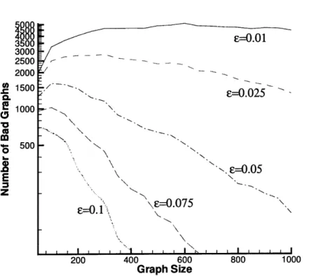
2.3 Number of graphs not satisfying Inequality (2.8) in 100,000 trials, for d = 4 and e = 0.01, 0.025, 0.05, 0.075, 0.1. . . . . 45

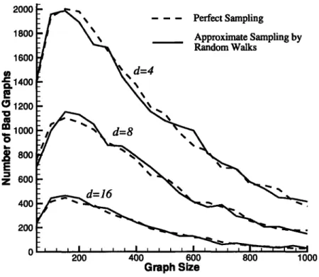
2.4 Number of graphs not satisfying Inequality (2.8) in 100,000 trials, for d = 4,8,16 and E = d/100. . . . . 46

3.1 A layered H-graph with d = 1. . . . . 76

4.1 A worst-case strongly-connected graph for Remark 46. . . . . 107

5.1 A Bluetooth scatternet. . . . . 122

5.2 Lines 5-7 in procedure CONNECTED for k = 7. . . . . 130

5.3 Lines 11-12 (IS(u) U S(w)I + 1 < k) in procedure CONNECTED for k = 7. . 131 5.4 Lines 13-15 (IS(u)I = 1) in procedure CONNECTED for k = 7. . . . . 131

5.5 Lines 16-21 (IS(u) U S(w)I + 1 = k) in procedure CONNECTED for k = 7. . 132 5.6 Lines 22-23 (default) in procedure CONNECTED for k = 7. . . . . 133

5.7 Number of piconets in the scatternet formed, compared to upper bound [(n - 2)/(k - 1)] + 1 and lower bound [(n - 1)/k], where k = 7. . . . . 141

5.8 Network diameter of the scatternet formed. . . . . 141

5.9 Number of rounds to form a scatternet. . . . . 142

5.10 Total number of Algorithmic Messages, Pages, and Inquiries. . . . . 143

5.11 Maximum number of Algorithmic Messages, Pages, and Inquiries sent by any single node. . . . . 143

5.12 Running time of the inquiry phase with three master-to-slave ratios. . . . . 145

5.13 Percentage of packet collisions (over all packets sent) when there are 50% masters and 50% slaves. . . . . 146

5.14 Running time of the page phase with three master-to-slave ratios. . . . . 146 5.15 Total number of packets sent when there are 50% masters and 50% slaves. . 147

List of Tables

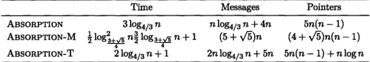
2.1 The expected number of replied messages generated by SAMPLE-BROADCAST. 31 2.2 The complexities of the sampling algorithms. . . . . 34 4.1 Performance of ABSORPTION, ABSORPTION-M, and ABSORPTION-T on

strongly-connected graphs. . . . . 116 4.2 Performance of NAME-DROPPER, KUTTEN-PELEG-VISHKIN, ABSORPTION,

and ASSIMILATION on three complexity measures. ... 119 4.3 Asymptotic bounds of strong-connecting algorithms. . . . . 119

Chapter 1

Introduction

Distributed algorithms can construct and alter network topologies efficiently. When network size increases, centralized topology control becomes difficult. This thesis introduces new distributed algorithms that change the connectivity of a topology and distributed algorithms that construct highly scalable topologies. To assist the topology construction algorithms, we also present several distributed algorithms that discover and collect information on these changing topologies. Applications of our algorithms include resource discovery, distributed hash tables, dynamic on-line communities, and topology construction for wireless ad hoc networks.

We will give an overview of the thesis in the rest of this Chapter. Section 1.1 motivates the construction of highly scalable expander networks. We preview the key theoretical results in Section 1.2 and applications in Section 1.3. Section 1.4 describes the structure of the thesis.

1.1

Motivations

1.1.1 Special Interest Networks

In this section we describe the main motivations behind our work on dynamic distributed algorithms.

Most existing peer-to-peer systems focus on distributed sharing of resources. They usu-ally facilitate sharing of storage (Napster, Gnutella, Freenet) or computation (SETI@Home). Many systems implement distributed hash tables.

Many believe that resource sharing is the major benefit of peer-to-peer networks. To facilitate resource sharing, a system usually needs to support resource searching. However, designing a scalable search system has always been very difficult.

Resource searching without any centralized directory usually suffers from poor perfor-mance when the number of participants grows. Distributed networks such as Gnutella

1.1. MOTIVATIONS

simply search by flooding the network and cannot provide any performance guarantee. A caching scheme such as the one employed by Freenet can replicate popular objects. However, less popular objects remain hard to be found.

A search system using a centralized directory requires a high-end machine to support a large network. Central directories are used by many established systems, such as ICQ, Napster, and SETI@Home. However, machines currently affordable by most individuals are unlikely to serve more than hundred thousand users. Although computers are getting cheaper and more powerful, the sizes of peer-to-peer networks and the amount of resource shared are also growing rapidly. Thus it is not clear whether a centralized server can serve a global peer-to-peer network in the near future.

We suggest that participants in peer-to-peer networks exhibit 'interest locality'. The resources a particular participant is interested in obtaining and sharing are correlated. For

example, in a file-sharing network, the file that a participant will download in the future is likely to be related to the files that she downloaded in the past. Consider the following scenarios:

* In a music-sharing network, participants would have preferences in different genres. For example, some participants could be interested in classical music but not pop music, or vice versa. In a global network, participants would have different language preferences too.

" In a file-sharing network, participants would have very different interests as well. Some are interested in text documents only. Some are looking for multimedia files. Also, users are usually interested in applications on specific platforms.

* In a general peer-to-peer network, participants usually have different goals. Some are interested in file-sharing, some are looking for fellow on-line gamers, some are looking for special interest discussion groups.

" In a heterogeneous environment, participants have different computing resources. Computing devices can range from mobile phones to enterprise servers. Certain appli-cations have delay constraints (action games), while others have bandwidth require-ments (large fie transfers).

In summary, it would be beneficial to peer with nodes of similar interests, instead of some arbitrary nodes.

We believe that a huge and all-purpose resource sharing network might not be necessary. Instead, we propose that different protocols can be used for "sharing" and "searching". We need large networks for searching so that we can potentially reach a large repository of resources. However, smaller networks are more efficient for most sharing activities. In other words, we mostly associate with smaller groups, we would like to be well-informed and have good 'connections' so that we can easily find and join other interesting groups. In order

1.2. THEORETICAL RESULTS

to reach such small groups easily, we would like to propose a protocol to connect as many nodes as possible, so that any such group can be formed and discovered efficiently.

Small groups of peer-to-peer networks can be tied by common interests. However, users need the means to search and reach the interest groups. We will present distributed algorithms that create and maintain special interest groups. Any interest group can be searched and reached with performance proportional to its size. We call this the Subset-Search problem because we want to search for a subset in a network.

In this thesis, we propose a collection of algorithms to solve the problem we have de-scribed. First, we need to scalable network to serve as a large search platform (Section 1.2.1). We need data collection algorithms to run on such dynamic network (Section 1.2.4). Then we need a hierarchical system to optimize for searches (Section 1.2.2). We also need an effective algorithm for special interest networks to be established (Section 1.2.3). We did an special study for this problem on wireless ad hoc networks (Section 1.3.3).

1.1.2 Distinctions

Subset-Search is different from group communications. Many distributed systems face scal-ability problems, especially if they support features such as anonymity, data security, and resistance to various attacks. Many features require the nodes to have a consistent view of the entire network, thus making any protocol difficult to scale to a large number of nodes. However, many applications do not need to satisfy these strong guarantees. For example, some video streaming applications can tolerate packet losses. In general, we can usually gain scalability by reducing requirements. We will design a protocol just strong enough to support Subset-Search.

Subset-Search is different from distributed hash tables. It is because a user typically does not have hashes of the objects that are interested to him or her. As an analogy, a web search engine user usually searches by keywords and other attributes, but will not know the hash or key of the relevant web pages.

Subset-Search is different from search engines. Machines in peer-to-peer networks are much more dynamic than most web servers.

1.2

Theoretical Results

We highlight the main theoretical contributions of this thesis. 1.2.1 Random Expander Networks

We present a novel distributed protocol for constructing an overlay topology based on ran-dom regular graphs that are composed of d > 4 independent Hamilton cycles. The protocol

1.2. THEORETICAL RESULTS

is completely decentralized as no globally-known server is required. The constructed topolo-gies are expanders with O(logd n) diameter with high probability.

Our construction is highly scalable because both the processing and the space require-ments at each node grow logarithmically with the network size. A new node can join the topology at any existing node in O(logd n) time with O(d logd n) messages. A node can leave in O(1) time with O(d) messages.

The analysis of our construction is based on a novel technique of studying a sequence of probability spaces. We also applied many results from random walks and random graphs.

1.2.2 Layered Expander Networks

H-graph is efficient for locating a member of a subset, when the size of the subset is not too small when compared with the size of the entire graph. However searching for a very small subset could be slow. For example, the expected time to find any particular node is 0(n).

We show that layered random regular graphs can be constructed such that each node has O(log n) neighbors and any node can be located in O(log n) steps given its identifier. We also present a variant that achieves degree-optimal routing at 0(logn/ loglogn) steps. We analyze the scheme where identifiers are assigned randomly and the scheme where identifiers are obtained by sampling in the existing graph. These recursively overlaid H-graphs are called layered H-graphs.

1.2.3 Resource Discovery and Connectivity

The problem of a network of computers discovering one another by making network con-nections is called the resource discovery problem. This problem was proposed by Harchol-Balter, Leighton, and Lewin [45]. The algorithmic task is to transform a weakly-connected graph into a complete graph by a distributed algorithm.

We present randomized algorithms to solve the resource discovery problem with 0(log n) time complexity and O(n2) expected message complexity. There are several variations of the algorithm with different tradeoffs in time and message complexities.

The problem of transforming a weakly-connected graph into a strongly-connected graph is also very interesting, and in fact might not be easier than the resource discvoery problem. We investigate several approaches to address this problem.

1.2.4 Algorithms on Dynamic Network Topology

We also study several interesting distributed algorithms on dynamic network topology. These algorithms have applications in our constructions in of H-graphs, but they are also of independent interests themselves. Most of the following algorithms depend on the expansion of the network graph to achieve good performance.

1.3. APPLICATIONS

Broadcasts and Searches

We present and analyze broadcast and search algorithms on random regular graphs that are composed of Hamilton cycles.

An important application of these algorithms is a service for the discovery of communities sharing common interests. Let A be a subset of nodes of a degree-d H-graph G such that

JAI /

IGI

0(i' + log n) hops in expectation even if set A is selected by an adversary.

Network Size Estimation

In a distributed network, any node does not easily know the size of the network. However, our construction algorithms would run more efficiently if we have a good estimation of the network size. Therefore, we would like to have an efficient distributed algorithm to gather and disseminate the size estimates.

Estimating the size of a network graph distributedly is an interesting algorithmic prob-lem. We propose a size-estimation algorithm based on random walks. With O(log n) walk-ers, we can obtain an fl(n) estimate at all nodes in O(n) time, with high probability.

1.3

Applications

We overview several applications of our distributed dynamic algorithms.

1.3.1

Distributed Lookup Service

A layered H-graph can be used to implement a distributed hash table similar to those

supported by Chord [921, CAN [83], Tapestry [991, and Pastry (85]. A lookup service stores key-value pairs in the network, such that the values can be looked up efficiently with the key. To implement a lookup service on the layered H-graph, keys can be hashed into identifiers.

A key is stored at the node whose identifier has the longest prefix match with the hashed

identifier. Insertions, deletions, and updates of entries have O(logn) time complexity and O(log n) message complexity. With optimizations, the time complexity can be improved to O(log n/log log n).

1.3.2

On-line Communities

A scenario where layered H-graph would be useful is a networked community where the

network address of a node may change from time to time. A layered H-graph construction can allow us to form an on-line community without any centralized directory. A node connected to the Internet by DHCP can have its IP address changed everyday. On a laptop

1.4. STRUCTURE OF THESIS

or PDA capable of local wireless access, the IP address can change even more frequently. A node changing its network address only needs to notify O(log n) other nodes in 0(1) time. Any node can reach another node in O(log n) hops given its identifier.

For example, a layered H-graph can be used to implement an on-line instant messaging system without any centralized server. Consider a student Ben chatting on-line during classes. If the on-line messaging system is implemented on a layered H-graph, then he only needs to notify O(logn) neighbor nodes when he moves to another classroom. When his friend Alice wants to obtain his new IP address after lunch break, she only needs to walk through O(log n) hops. Such feature is not easy implement on distributed systems because if Alice and Ben have overlapping lunch breaks, they would have difficulty finding each others' IP addresses in the afternoon.

1.3.3 Bluetooth Topology Construction

A Bluetooth ad hoc network can be formed by interconnecting piconets into scatternets. The

constraints and properties of Bluetooth scatternets present special challenges in forming an ad hoc network efficiently. In Chapter 5, we present and analyze a new randomized protocol for Bluetooth scatternet formation.

We prove that our algorithm achieves O(log n) time complexity and 0(n) message com-plexity. The scatternets formed have the following properties: 1) any device is a member of at most two piconets, and 2) the number of piconets is close to be optimal. These proper-ties can help prevent overloading of any single device and lead to low interference between piconets.

We validate these theoretical results by simulations. In addition, the simulations show that the scatternets formed have O(log n) diameter.

As an essential part of the scatternet formation protocol, we study the problem of device discovery: establishing multiple connections simultaneously with many Bluetooth devices. We investigate the collision rate and time requirement of the inquiry and page processes.

Deducing from the simulation results of scatternet formation and device discovery, we show that the total number of packets sent is O(n) and that the maximum number of packets sent by any single device is O(log n).

1.4

Structure of Thesis

In Chapter 2, we present and analyze the construction of the random expander networks. In Chapter 3, we construct layered networks of random expanders to implement a fast dis-tributed lookup service. Chapter 4 describes disdis-tributed algorithms for resource discovery. Chapter 5 presents an application of the topology construction methodology in wireless ad hoc networks. We conclude and discuss future work in Chapter 6.

Chapter 2

Construction of Expander

Networks

2.1

Introduction

The area of peer-to-peer networking has recently gained much attention in both the in-dustry and the research community. Well-known peer-to-peer networks include Napster, Gnutella, Freenet, FastTrack, and eDonkey. However, most of these systems either require a centralized directory or cannot scale beyond a moderate number of nodes. The problem of finding an efficient distributed scalable solution has attracted a lot of research interests [83, 92, 85, 99]. This chapter introduces a distributed algorithm for constructing expander networks, which are suitable for peer-to-peer networking, without using any globally-known server.

Interesting properties and algorithms have been discovered for random regular graphs [34, 36, 37, 58]. In particular, it has been found that random regular graphs are expected to have big eigenvalue gaps [32] with high probability, and thus are good expanders.

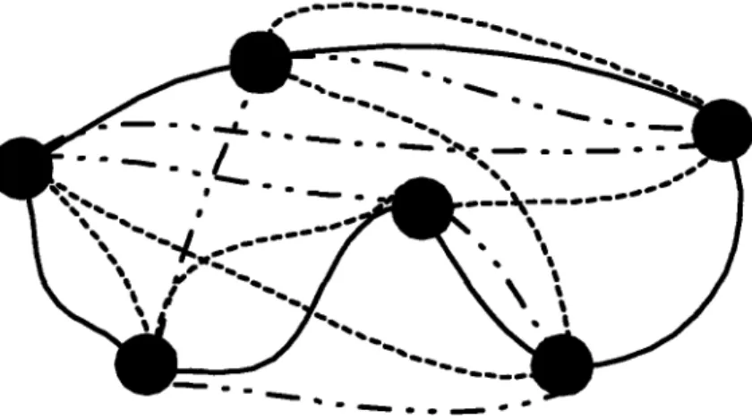
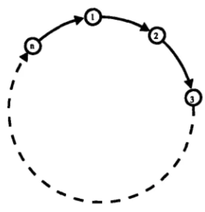
In this chapter, we form expander graphs by constructing a class of regular graphs which we call H-graphs. An H-graph is a 2d-regular multigraph in which the set of edges is composed of d Hamilton cycles (Figure 2.1 is an example). Using random walk as a sampling algorithm, a node can join an H-graph in O(logd n) time with O(d logd n) messages, and leave in 0(1) time with O(d) messages.

Section 2.2 describes our network model and gives an overview of the design of H-graphs. Section 2.3 introduces the protocol for constructing H-graphs. We discuss several perfect sampling algorithms in Section 2.4 and a random-walk sampling algorithm in Section 2.5, with simulation results in Section 2.6. Two useful maintenance algorithms are discussed in Section 2.7. We discuss broadcasts in Section 2.8 and searches in Section 2.9. Then we study distributed network size estimation in Section 2.10. At last, fault tolerance issues

2.2. PRELIMINARIES

Figure 2.1: An H-graph consisting of 3 Hamilton cycles.

are discussed in Section 2.11. We discuss related work in Section 2.12 and conclude with remarks on future work in Section 2.13.

2.2

Preliminaries

In this section, we will state our assumptions of the underlying network model and then describe the goals and constraints that lead to our design based on random regular graphs.

2.2.1 Network Model

We assume a network environment where any node u can send a message to node v as long as node u knows the address of v. If a node fails to receive a message for whatever reason, the sending node can repeat sending the message without causing the algorithm to fail. There can be node failures but not permanent link failures. Such model is assumed in [45] and most peer-to-peer research. An example of such an underlying network is the Internet when using some reliable messaging protocol such as TCP.

The space requirement will be expressed in the number of addresses. Theoretically, O(log N) bits are required to encode the address of a node, where N is the largest possible number of nodes. However, for all practical purposes, we can assume that the length of an

address is effectively constant (e.g., 128 bits in IPv6).

We assume that there is a maximum delay between all pairs of nodes in the underlying network. In practice, the processing time per message is usually insignificant compared to

2.2. PRELIMINARIES

the communication time. Also, for a small message, the delivery time is mostly independent of the message size.

Each execution of a distributed algorithm will lead to a set of messages sent among the nodes in the graph. The message complexity of an algorithm is the size of this set. Some of these messages have causal relationships: there is some sequence M1, m2,... of

messages where mi cannot be sent before mi._1 has been received. We will express the time

complexity of an algorithm as the length of the longest such sequence.

We will be concerned with the logical topologies overlaid on top of the underlying network. On a set of nodes with labels [n] = {1,2,...,n}, a topology can be effectively determined by sets of neighbors N(u), which are nodes known to node u (not including u itself), for u

E

(u, v) E E iff v c N(u).

We consider distributed algorithms on the graph such that u can send a message to v only if (u, v) E E. During the execution of our algorithm, an edge (u, v) can be added into

E if u is informed of the address of v. Node u might also choose to delete (u, v) for some v

to save space.

2.2.2 Goals and Requirements

Our first goal is to construct logical topologies that can support broadcasting and searching efficiently. Our second goal is to make our construction highly scalable. This implies the objectives:

A-1 Resources consumed at each individual node should be as low as possible. A-2 Time complexities for joining and leaving of nodes should be as low as possible.

A key factor on the load of a node is the number of nodes that it has to communicate with. This parameter determines a node's minimum storage requirement and the maximum number of potential simultaneous network connections. The number of neighbors of a node is its degree in the graph. Therefore, objective A-1 dictates that the degrees should be as small as possible. In order to achieve objective A-2, we need to make sure that the algorithms for nodes joining and leaving are efficient.

2.2.3 A Random Graph Approach

To make worst-case scenarios unlikely, we have decided to construct the graph with a randomized protocol. We would like our topology to be 'symmetric' in the sense that every node shares an equal amount of responsibilities. For this reason and for providing better

2.2. PRELIMINARIES

fault tolerance, we did not choose a hierarchical approach. After considering various random graph models, we chose regular multi-graphs that are composed of independent Hamilton cycles. Regular graphs are chosen because we would like the degree to be bounded. Also, random walking on regular graphs, which is a key part of our protocol, has a uniform stationary distribution. Graphs composed of Hamilton cycles have the advantage that the join and leave operations only require local changes in the graph.

Now we shall define the set of H-graphs. Let H, denote the set of all Hamilton cycles on set [n]. We shall assume n > 3 for rest of this paper. Consider a multigraph G = (V, E), such that V = [n] and E = (C1,. .. , Cd), where C1, C2,. .., Cd E Hn. Let Hn,2d be the set

of all such 2d-regular multigraphs. We call the elements in Hn,2d the H-graphs. It can be derived that

IHnI

uniform samples of Hn, then (V, (C1, ... , Cd)) is a uniform sample of Hn,2d.

Following the notation in Bollob6s [161, a probability space is a triple (Q, E, P), where

Q is a finite set, E is the set of all subsets of S, and P is a measure on E such that P(fl) = 1

and P(A) = ZWEA P({w}) for any A E E. In other words, P is determined by the values of P({w}) for w E Q. For simplicity, we will write P(w) for P({w}).

Let Un be the uniform measure on set 11 so that Un {w} = 1/ 01 for all w E Q. For

example, we have UH, 2d {G} = (2/(n - 1)!)d for all G E Hn,2d.

We shall consider two basic operations for a randomized topology construction protocol: JOIN and LEAVE. A JOIN(u) operation inserts node u into the graph. Any node in G should be able to accept a JOIN request at any time. Any node in G can also call LEAVE to remove itself from the graph G. Our algorithms of JOIN and LEAVE are described in Section 2.3. Given an initial probability space So and a sequence of JOIN and LEAVE requests, a randomized topology construction protocol will create a sequence of spaces

S1, S2 . .

Friedman [32, 33] showed that a graph chosen uniformly from Ha,2d is very unlikely to

have a large second largest eigenvalue. In order to apply Friedman's theorem, we need a protocol that would produce a sequence of uniformly distributed spaces.

Given a probability space S = (f', E', P'), let Q[S] = 0' and P[S] = P'. A probability

space S is uniformly distributed if P[S] = UQ[S]. We would like to have a protocol that

creates a sequence of uniformly distributed probability spaces, given any sequence of JOIN and LEAVE requests. In addition, a new node should be free to call JOIN at any existing node in the graph.

Summarizing the objectives we have so far, we would like to have a protocol where B-1 Low space complexity at any node.

B-2 Low time complexities for JOIN and LEAVE. B-3 Low message complexities for JOIN and LEAVE.

2.3. CONSTRUCTION

B-4 The probability spaces produced are uniformly distributed.

Satisfying the first three properties is crucial because they are necessary for our protocol to be highly scalable. When property B-4 is not satisfied, we can try to construct sequences of probability spaces So, S,.... having distributions close to be uniform. This can be achieved by an algorithm based on random walks presented in Section 2.5. We have yet to find a protocol satisfying all four properties simultaneously.

2.2.4 Global Variable Server

We will also consider variants where a globally-known server can simplify the algorithm or enhance the performance. We call such server a global server, whose address is known to all nodes in the graph. The global server should be reliable and highly available. We note that similar servers are assumed in most related work [77, 57] of randomized network constructions.

We will restrict our attention to those protocols that require the global servers to store O(1) addresses. In other words, a global server implements O(1) global variables that are visible to all nodes in the graph. The size of each variable is limited to O(log n) bits. We assume that atomic updates of the variables are ensured by the global server. A global server can be implemented as a cluster.

In summary, although the global server requires extra reliability, it does not need ex-traordinary storage, processing, or communication capacity.

2.3

Construction

In this section we introduce a framework for constructing a random regular network. The graphs that we shall construct are 2d-regular multigraphs in Hn,2d, for d > 4. The neighbors of a node are labeled as

ngbr_1, ngbrl, ngbr-2, -.. , ngbr-, ngbrd.

For each i, ngbr_; and ngbri denote a node's predecessor and successor on the ith Hamilton cycle (which will be referred to as the level-i cycle).

We start with 3 nodes, because there is only one possible H-graph of size 3. In practice, we might want to use a different topology such as a complete graph when the graph is small. The graph grows incrementally when new nodes call JOIN at existing nodes. Any node can leave the graph by calling LEAVE.

In the following algorithmic pseudocodes, the variable self identifies the node executing the procedure. All the actions are performed by self by default. The expression u =*PROc()

invokes a remote procedure call PRoc at node u. The call is assumed to be non-blocking unless a return value is expected. Expression u =* var means that we request the value var

2.3. CONSTRUCTION

from node u. Expression (u => var) <- x means that we set the variable var of node u to value x. Thus, messages are exchanged between node self and node u.

Procedure LINK connects two nodes on the level-i cycle.

LINK(u, v, i)

1 (u -ngbr;) <- v 2 (v => ngbr;) +- u

Procedure INSERT(u, i) makes node u the successor of self on the level-i cycle. We assume that INSERT is atomic. This can achieved by having a lock for each of the d Hamilton cycles at each node.

INSERT(U, i)

1 LINK(u, ngbri, i) 2 LINK(self, u, i)

A new node u joins by calling JOIN(u) at any existing node in the graph. Node u will be inserted into cycle i between node vi and node (vi => ngbr;) for randomly chosen vi's for i =1,...,d.

JOIN(U)

1 for i+- 1,...,d in parallel 2 do vi +- SAMPLEO

3 for i+- 1,...,d in parallel 4 do vi = INSERT(u, i)

SAMPLEO

1 return a node in the graph containing self, uniformly at random

Procedure SAMPLEO returns a node of the graph chosen uniformly at random. Imple-mentations of SAMPLE are presented in Section 2.4.

LEAVE(0

1 for i<-- 1,...,din parallel 2 do LINK(ngbr_ , ngbr, i)

We first show that JOIN can preserve uniform probability spaces.

Lemma 1. Let (En_1,2d, E, P) be a uniformly distributed probability space. After an oper-ation JOIN, the probability space (Hn,2d, V', P') is also uniformly distributed.

2.3. CONSTRUCTION

Proof. Let G = (V, E) be a uniformly random graph from IHI-1,2d. Let G' = (V', E') be

the graph obtained after a JOIN operation. Let Ei and Ej be the set of level-i edges in E and E' respectively, for i = 1, .. ., d.

We need to show that each (V', Ej) is an independent Hamilton cycle chosen from H, uniformly. Procedure SAMPLE returns a node chosen from V uniformly at random. This means that it is equally likely that the new node is inserted between any pair of nodes in the cycle (V, E). Therefore, since (V, Ei) is a uniformly random Hamilton cycle in H,_-,

(V', Ej) will be a uniformly random Hamilton cycle in H,.

Since the d calls to SAMPLE are independent, the Hamilton cycles (V', Ej) are

indepen-dent. E

By Lemma 1, we can expect to obtain a uniform probability space if we remove the node

that has just joined. However, if the space is uniform, the nodes should not be differentiable

by the order of joining. Thus, Lemma 2 shows that the probability space remains uniformly

distributed no matter which particular node leaves.

Lemma 2. Let (1HIn,2d, E, P) be a uniformly distributed probability space. After an operation LEAVE at any node in G, the probability space (Hn-1,2d, E', P') is also uniformly distributed.

Proof. Let G be a uniform sample from Hn,2d. We can consider each Hamilton cycle in G separately. Consider any particular level-i cycle of G. Let j be the node calling LEAVE. Given j, there are

("2)

j.

(n21)

Consider the map o-: ELn 1- H'_1, where H'_ 1 is the set of all cycles on

{ ,..., 1 + ,...,n},

such that a(C) is obtained by removing node

j

Let o--1(C') = {C E Hn I o(C) = C'}. Consider any graph C' E H'-_1. If (u, v) V E(C'), then o -'(C)

n

a (C)

U

Hu,,

(u,v)EE(C)

For each adjacent pair {u, v} of neighbors in C,

|o-

_n

by removing

j

j.

2.4. PERFECT SAMPLING

Since each graph in H, has probability 2/(n - 1)!, each graph in H,_1 has probability

(n -- 1)(2/(n -- 1)!) = 2/(n - 2)!.

Since the d cycles are independent of each other, P'(G) = (2/(n - 2)!)d for any G E

Hn-1,2d. Thus, (Hn-1,2d, F', P') is uniformly distributed.

Theorem 3. Let So, S1, S2,... be a sequence of probability spaces such that

" So is uniformly distributed and 92[So] = H k,2d for some k; " S,+j is formed from Si by JOIN or LEAVE;

" |Q[Sj]| I 3 for all i > 0.

Then Si is uniformly distributed for all i > 0.

Proof. We start with a H-graph of size 3. We note that 1H3,2dl = 1, thus the initial

probability space So has uniform distribution. The theorem then follows from Lemma 1

and Lemma 2 by induction. E

A graph G of size n has a corresponding n by n matrix A, in which the entry Aj is

the number of edges from node i to node j. Let A(G) be the second largest eigenvalue of graph G's matrix. Friedman [32] showed that random regular graphs have close to optimal

A(G) with high probability. Although he mainly considered the graphs that are composed

of d random permutations, he also showed that his results hold for graphs composed of d random Hamilton cycles. Theorem 4 restates a recent improvement by Friedman [33].

Theorem 4 (Friedman). Let G be a graph chosen from H,,2d uniformly at random. For any e > 0,

A(G) < 2V2d -1+ e with probability 1 - O(n-'), where -r =

[v(d--

It has been known that A(G) 2vW2d-- + 0(1/logdn) for any 2d-regular graph. Therefore, no family of 2d-regular graphs can have smaller asymptotic A(G) bounds than Theorem 4.

As a consequence of Theorem 4, H-graphs are expanders with O(logd n) diameter with high probability because of the relation between eigenvalues and expanders [7, 52].

Let p(G) = A(G)/A(G) for regular graph G of degree A(G). We note that p(G) is the second largest eigenvalue of the Markov chain with transitions based on G.

2.4

Perfect Sampling

2.4. PERFECT SAMPLING

2.4.1 Global Server

In a simple centralized solution using a publicly-known sampling server, each joining node can obtain d uniformly random nodes from the sampling server. Each JOIN or LEAVE operation only takes 0(1) time and 0(1) messages. The space required at the sampling server is 0(n).

The sampling server sampleserver keeps the addresses of all nodes of the network.

SAMPLE-CENTRAL()

1 return sampleserver => RANDOM-NODE)

RANDOM-NODESO

1 _{return UNIFORM(G)}

This process take 0(1) time and 2d messages. We can also easily combine those 2d messages into a single query. Whenever a node is added or removed from the network,

0(1) maintenance messages are required. The space (number of addresses) required at the

sampling servers are 0(n).

This is a simple and efficient solution. However, it subjects to most of the disadvantages of a centralized solution. For example, we need to have a complete trust on the sampling server returning unbiased samples of the network. We also need to have a reliable public source for the server's address.

Although this solution is subject to most disadvantages of centralized systems, it is still better than a fully centralized solution because only an address list is stored at the sampling server. It is not required to store any description of the nodes, as searching is still distributed. Thus the load on the sampling server only depends on the rate of topology changes but not the search queries and other algorithms running on the network.

2.4.2 Broadcast

Instead of using a central server, a joining node can broadcast a request to all other nodes. Each node is asked to reply with a chosen probability p = 0(1/n). Thus the joining node can expect to receive 0(1) replies and then pick one as the sample. A broadcast on an H-graph sends at most (2d - 1)n messages and terminates in O(logd n) steps with high probability (Section 2.8).

The procedure SAMPLE-BROADCAST calls the generic service BROADCAST (Section 2.8) so that SAMPLE-PROC is executed once on every node of the graph. Parameter p is the probability of replying.

2.4. PERFECT SAMPLING

Procedure SAMPLE-BROADCAST needs an estimation of logn. Estimation algorithms are discussed in Section 2.10.

In procedure SAMPLE-PROC, the set I keeps the set of levels (Hamilton cycles) that a node decides to respond to. Set I is a subset of {1, ... , d} such that for each i E {1, .. . , d},

i E I with probability p.

The replies are then aggregated at the variables Si at the source node s. The probability that any set Si is empty is (1 - p)". The probability that all sets Si are non-empty is

(1 - (1 - p)n)d. Thus, in expectation, (1 - (1 - p)n)-d rounds of broadcast are needed. The probability that a node calls the broadcast source s with SAMPLEREPLY is 1 (1

-p)d. Thus the source

s

bxpd.

of broadcast. The overall expected number of reply messages is flj(j. Let p = /3/n.

For large n, - (1 -p)d dO (1-(1 - p)n) ( -e-)d ' SAMPLE-BROADCAST(p) 1 repeat 2 S1- S2 S--- Sd+-0d

3 P <- NEW (SAMPLE-PROC, {s +-- self, p <- p})

4 BROADCAST(P)

5 SLEEP(E(logn))

6 until min1i<sd ISi > 0 7 S -0 8 for i <- 1 to d 9 do S +- S U UNIFORM(Sj) 10 return S SAMPLE-PROC() 1 locals s, p 2 I+-0 3 for i +-1 to d 4 do I +- I U i with probability p 5 if I0 0 6 then S =- SAMPLE-REPLY(self, I) 7 return true SAMPLE-REPLY(U, I) 1 foriEI 2 doSi -SiUu

2.4. PERFECT SAMPLING

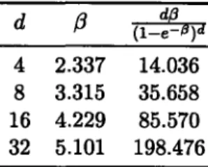
4 2.337 14.036

8 3.315 35.658 16 4.229 85.570 32 5.101 198.476

Table 2.1: The approximate optimal values of

3

of replied messages generated by SAMPLE-BROADCAST.

Therefore, it is possible to select the parameter p so that the expected total number of reply messages is a function of d. The function d- is minimized when e# -1 = #d. Table 2.1 gives the optimal values of

3

2.4.3 Converge-Cast

In the worst case, the source node has to handle O(n) replies resulting from a broadcast. We note that a broadcast can construct a 0(log n)-depth spanning tree in O(log n) time. Instead of asking each node to reply independently, a protocol can 'combine' the sampling results at the internal nodes of the spanning tree, so that each node only needs to handle O(d) messages in the worst case.

SAMPLE-SPANNING(PROC, nonce h)

1 if h was seen recently

2 then return NULL

3 for each v E N(self) in parallel

4 do S - S U {v => SAMPLE-SPANNING(PROC, h)} 5 z -self

6 t- 1

7 for each (z', t') in S 8 do t <- t + t'

9 with probability t'it

10 then

z <-

11 return (z,t)

Theorem 5. Procedure SAMPLE-SPANNING returns each node in the graph G with proba-bility 1/ GI.

Proof. First, we observe that SAMPLE-SPANNING establishes a spanning tree rooted at the initial node. Thus, we only need to show that in any subtree T rooted at node v, each node in T is returned with probability 1/ ITI.

2.4. PERFECT SAMPLING 1000 - 800-U) ca E 600-0) E 400-Cu E E E 200-00 20 40 60 80 160 120

Figure 2.2: The minimum expected number of reply messages received in

2.5. APPROXIMATE SAMPLING

For the base case, a leaf has to return itself with probability 1. Inductively, let T1, ... , Tk

be the subtrees of v so that the f or loop in SAMPLESPANNING goes through these trees in order of T1, ... , Tk. Let z' be the node returned by subtree T. In the ith iteration of the

f or loop, there is a probability of that z' replaces the existing value of variable z. And the probability that z' is not replaced in loop j > i is 4F<1jz4TI. Therefore, the probability that z' is returned by v => SAMPLESPANNING is

ITi1 1

+

E,

i ITIj

E1<L<k1

1

+ E1<<

+

Ei<i+i

T1

EX<l<k

UII

ITi I

1 + Zi<1<k

KII

ITI

Since each node in Ti is selected with probability 1/

IT

I

node in T will be returned by v with probability 1/ TI. It is straightforward to verify that

v itself is returned with probability 1/ JT. ]

We note that SAMPLE-SPANNING is a broadcast together with information aggregation along the broadcast tree from the leaves to the root. Therefore, it has O(logdn) time complexity and O(dn) message complexity.

2.4.4 Coupling From The Past

Perfect sampling algorithms for Markov chains have been discovered in recent years. Lovisz and Winkler [68] gave the first exact sampling algorithm for unknown Markov chains. Propp and Wilson [81] introduced faster algorithms based on their 'coupling from the past' (CFTP) procedure. They gave an algorithm COVER-CFTP which generates a state dis-tributed with stationary 7r in expected time at most 15 times the cover time. The expected cover time for H-graphs is around n log n [6] with high probability. Thus the running time

of COVER-CFTP on an H-graph is O(nlogn). It is not clear if a faster CFTP algorithm can be found by discovering a monotone coupling [80].

2.5

Approximate Sampling

The sampling algorithms in Section 2.4 are either centralized or require f2(n) messages, and thus are not satisfactory for our goal of efficient and distributed construction. The existence of a distributed perfect sampling algorithms for regular graphs with o(n) message complexity is an open problem.

2.5. APPROXIMATE SAMPLING

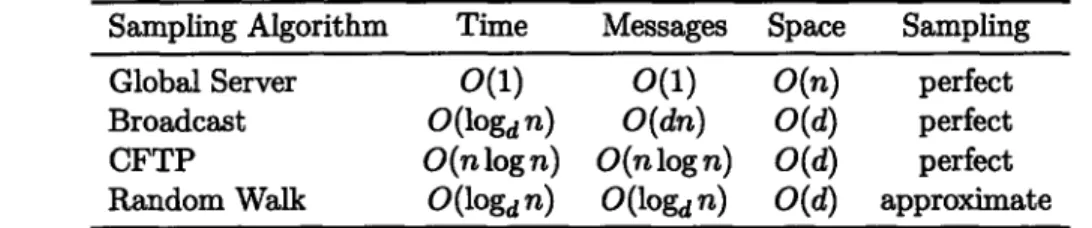
Sampling Algorithm Time Messages Space Sampling

Global Server O(1) O(1) O(n) perfect

Broadcast O(logd n) O(dn) O(d) perfect

CFTP O(nlogn) O(nlogn) O(d) perfect

Random Walk O(logd n) O(logd n) O(d) approximate

Table 2.2: The complexities of the sampling algorithms. "Space" is the worst-case storage requirement at any node.

In this section, we describe an approach for approximate sampling using random walks. A graph can be considered as a Markov chain. Sampling by random walks is usually called Markov Chain Monte Carlo [48]. Since H-graphs are regular, the limiting distribution of random walks on H-graphs is the uniform distribution. Moreover, since an H-graph is an expander with high probability, a random walk of 0(logn) steps on an H-graph can sample the nodes of the graph with a distribution close to be uniform. We shall show that our protocol with approximate sampling increases the probability of producing 'bad graphs' (those with large A(G)) by only a constant factor. Therefore, if the graph is sufficiently large, the high probability result of Theorem 4 can still be applied. With approximate sampling, we need to start with a uniformly distributed probability space of sufficiently large graphs. When the graph is small, we can use a perfect sampling algorithm described in Section 2.4.

Procedure SAMPLE-RW(t) performs a random walk on the graph and returns the node after t steps.

SAMPLE-RW(t) 1 if t=O

2 then return self

3 else v +- a random element in N(self) 4 return V => SAMPLE-RW(t - 1)

Procedure SAMPLE-RW is presented here as a tail recursion through remote procedure calls. We can as well pass along the network address of the initial node. Procedure SAMPLE-RW can serve as an implementation of SAMPLE in Section 2.3. The variant of JOIN using SAMPLE-RW will be denoted as JOIN-RW. Table 2.2 summarizes the complexities of the sampling algorithms we have considered.

2.5.1 Nodes Joining

We now analyze the sequence of probability spaces of H-graphs generated by the JoIN-RW operations. Lemmas 6 and 7 are consequences of Theorem 5.1 in [67].

2.5. APPROXIMATE SAMPLING

Lemma 6. If G is a k-regular graph of size n, then for any i E G,

Pr {SAMPLE-RW(t) returns i} - - (

Proof. By Theorem 5.1 of [67], we have

IPt(j)

-

P ,

where p = f Since ir(j) = 7r(i) = 1/n for all ij, = 1.

Lemma 7. Let G

E

log C

t= [ r =io 0 (logd n)

[log

where r and c are positive constants. Then for any v

E

Pr {SAMPLE-RW(t) returns v} - - .

In dnr

Proof. Let p = 2v 1+c and t* = log,/, dnr/c. By Lemma 6, if t > t*, then pt 5 c/dnr. E

Theorem 8 shows that although our protocol using SAMPLE-RW does not sample per-fectly, the probability that we obtain a graph of large second eigenvalue remains very small. Theorem 8. Let d > 3. Let Sn, Sn+1, Sn+2,... be a sequence of probability spaces where

Sk = (Hk,2d, Ek, Pk). Let Sn be a uniformly distributed probability space and let Sk+1 be

formed from

21 + r > 2. Then for all k > n,

Pk{ G

E Hk,2d

I

}

Proof. Let Tn =

{

}

Let J(G) be the set of graphs obtained by operation JOIN (it does not matter whether we consider JOIN or JOIN-RW) on G. For any k > n, let

2.5. APPROXIMATE SAMPLING

The probability space Sk can be considered as a product space (Ck)d where Q [Ck] = Hk.

For any C E Hk and I E {1,.. ., d}, let

Hk [1, C] ={ G E Hk,2d I C is the level-I Hamilton cycle of G

}

be the set of graphs whose level-I cycle is C.

For any probability space (0, E, P) and any sets A, B C Q, let

P{A

I

n

Pm {Tm} ZeO(~7), %1=- (2.2)

and

sup Pm { Hm[1, C]

I

CEHm (m - 1)!/2

1<L<d

Because of our assumption that Sn is a uniformly distributed probability space and Theorem 4, Pn {T} _> 1 - O(n-T). The eigenvalue of a graph depends on the structure of the graph but not the labels. In other words, a graph has the same eigenvalue no matter how we label the nodes. Thus, we have

1 Pn Hn [1, C] I Tn } = Pn {Hn [1, C]}=(D ₂ Therefore, Inequalities (2.2) and (2.3) are satisfied for the base case m = n.

Assuming that Inequalities (2.2) and (2.3) are satisfied for m = k, we shall show that

they are satisfied for m = k + 1.

Let t(k, d)= log be the number of steps walked by SAMPLE-RW.

log ;dd

The set J(Tk) are those graphs that can be produced by an operation JOIN on the graphs in Tk. Let C' E Hk be the cycle such that node k + 1 is removed from a cycle

C E Hk+1. A graph in Hk+1[l, C] n J(Tk) must be created by inserting the node k + 1 at

level I between two nodes of a graph in Hk [1, C'] n Tk. We have

sup Pk+1 { Hk+ 1[, C] IJ(Tk)} CEHk+1, 1<l<d

< sup Pk{Hk[l,C']ITk}x C'EHk, 1<1<d

sup Pr {SAMPLE-RW(t(k, d)) on G returns v}. vEk],GETk

2.5. APPROXIMATE SAMPLING

Let

sup Pr {SAMPLE-RW(t(k, d)) on G returns v} = 1/k + Ek. vE[k],GETk

Informally, Ek is the amount of deviation resulted from the approximate sampling on some G E Tk by a random walk. It would be zero if a perfect sampling algorithm is used. By

Lemma 7, Ek 5 '. By the inductive assumption of Inequality (2.3) of m = k, we have

sup Pk+1 {Hk+1[l, C] Tk+1

}

I

~+)-i

sup Pk+1 { Hk+1[1, C] I Tk+1

}

}

CEHk+1, 1<1<d CEHk+l, 1<1<d

Thus Inequality (2.3) is satisfied for m = k + 1.

Since a new node is inserted into the d Hamilton cycles independently during each JOIN

operation, we have sup Pk+{CI

G

J

Dividing both sides by UHk+1 2d {G}, we have

sup Pk+i

{