An Application of Multi-band Forced Photometry to One Square Degree of SERVS: Accurate Photometric Redshifts and Implications for Future Science

HAL Id: hal-01582761

https://hal.archives-ouvertes.fr/hal-01582761

Submitted on 9 May 2018

HAL is a multi-disciplinary open access

archive for the deposit and dissemination of

sci-entific research documents, whether they are

pub-lished or not. The documents may come from

teaching and research institutions in France or

abroad, or from public or private research centers.

L’archive ouverte pluridisciplinaire HAL, est

destinée au dépôt et à la diffusion de documents

scientifiques de niveau recherche, publiés ou non,

émanant des établissements d’enseignement et de

recherche français ou étrangers, des laboratoires

publics ou privés.

An Application of Multi-band Forced Photometry to

One Square Degree of SERVS: Accurate Photometric

Redshifts and Implications for Future Science

Kristina Nyland, Mark Lacy, Anna Sajina, Janine Pforr, Duncan Farrah,

Gillian Wilson, Jason Surace, Boris Häußler, Mattia Vaccari, Matt Jarvis

To cite this version:

Kristina Nyland, Mark Lacy, Anna Sajina, Janine Pforr, Duncan Farrah, et al.. An Application of

Multi-band Forced Photometry to One Square Degree of SERVS: Accurate Photometric Redshifts and

Implications for Future Science. Astrophys.J.Suppl., 2017, 230 (1), pp.9. �10.3847/1538-4365/aa6fed�.

�hal-01582761�

Typeset using LA_{TEX twocolumn style in AASTeX61}

AN APPLICATION OF MULTI-BAND FORCED PHOTOMETRY TO ONE SQUARE DEGREE OF SERVS: ACCURATE PHOTOMETRIC REDSHIFTS AND IMPLICATIONS FOR FUTURE SCIENCE

KRISTINANYLAND,1_M ARKLACY,1_A NNASAJINA,2_J ANINEPFORR,3, 4_D UNCANFARRAH,5_G ILLIANWILSON,6_J ASONSURACE,7

BORISHÄUSSLER,8MATTIAVACCARI,9, 10ANDMATTJARVIS9, 11

1_{National Radio Astronomy Observatory, Charlottesville, VA 22903, USA} 2_{Department of Physics & Astronomy, Tufts University, Medford, MA 02155, USA} 3_{ESA/ESTEC SCI-S, Keplerlaan 1, 2201 AZ, Noordwijk, The Netherlands}

4_{Aix Marseille Université, CNRS, LAM (Laboratoire d’Astrophysique de Marseille) UMR 7326, 13388, Marseille, France} 5_{Department of Physics, Virginia Tech, Blacksburg, VA 24061, USA}

6_{Department of Physics and Astronomy, University of California-Riverside, 900 University Avenue, Riverside, CA, 92521, USA} 7_{Spitzer Science Center, California Institute of Technology, M/S 314-6, Pasadena, CA 91125, USA}

8_{European Southern Observatory, Alonso de Cordova 3107, Vitacura, Casilla 19001, Santiago, Chile}

9_{Department of Physics and Astronomy, University of the Western Cape, Robert Sobukwe Road, 7535 Bellville, Cape Town, South Africa} 10_{INAF - Istituto di Radioastronomia, via Gobetti 101, 40129 Bologna, Italy}

11_{Department of Physics, Oxford Astrophysics, University of Oxford, Keble Road, Oxford OX1 3RH, UK}

(Accepted 4/11/2017) Submitted to ApJS

ABSTRACT

We apply The Tractor image modeling code to improve upon existing multi-band photometry for the Spitzer Extragalactic Representative Volume Survey (SERVS). SERVS consists of post-cryogenic Spitzer observations at 3.6 and 4.5 µm over five well-studied deep fields spanning 18 deg2_{. In concert with data from ground-based near-infrared (NIR) and optical surveys,}

SERVS aims to provide a census of the properties of massive galaxies out to z ≈ 5. To accomplish this, we are using The Tractor to perform “forced photometry.” This technique employs prior measurements of source positions and surface brightness profiles from a high-resolution fiducial band from the VISTA Deep Extragalactic Observations (VIDEO) survey to model and fit the fluxes at lower-resolution bands. We discuss our implementation of The Tractor over a square degree test region within the XMM-LSS field with deep imaging in 12 NIR/optical bands. Our new multi-band source catalogs offer a number of advantages over traditional position-matched catalogs, including 1) consistent source cross-identification between bands, 2) de-blending of sources that are clearly resolved in the fiducial band but blended in the lower-resolution SERVS data, 3) a higher source detection fraction in each band, 4) a larger number of candidate galaxies in the redshift range 5 < z < 6, and 5) a statistically significant improvement in the photometric redshift accuracy as evidenced by the significant decrease in the fraction of outliers compared to spectroscopic redshifts. Thus, forced photometry using The Tractor offers a means of improving the accuracy of multi-band extragalactic surveys designed for galaxy evolution studies. We will extend our application of this technique to the full SERVS footprint in the future.

Keywords:catalogs – methods: data analysis – surveys – techniques: image processing – Galaxies: evolution

Corresponding author: Kristina Nyland knyland@nrao.edu

1. INTRODUCTION AND MOTIVATION

Beginning with the successful SIRTF Wide-area Infrared Extragalactic Legacy Survey (SWIRE;Lonsdale et al. 2003) over a decade ago, a growing number of deep extragalac-tic surveys with the Spitzer Space Telescope (Werner et al. 2004) have provided unprecedented insights into the evo-lution of galaxies over cosmic time. Although the SWIRE footprint spanned ∼49 deg2 _{and included imaging in seven}

Spitzerbands from the near- to far-infrared, it was primar-ily sensitive to objects at low and intermediate redshifts of z. 3 due to its relatively shallow depth. More recently, the abundance of post-cryogenic observing time with Spitzer for large programs has made the construction of wide-area deep fields more feasible in the shortest two bands of the Infrared Array Camera (IRAC;Fazio et al. 2004) that have remained in operation. This has been particularly fortuitous for galaxy evolution studies since the combination of the in-herent shapes of galaxy spectral energy distributions (SEDs) and the low background level in the IRAC bands make IRAC uniquely well-equipped for the detection of high-redshift galaxies given sufficient exposure time (e.g., Oesch et al. 2014). Furthermore, until the launch of the James Webb Space Telescope (JWST) currently scheduled for late 2018, IRAC is one of the few instruments capable of detecting rest-frame optical emission from galaxies at z > 4.

A number of recent surveys have capitalized on the op-portunity to conduct deep, wide-area IRAC surveys at 3.6 and 4.5 µm during the warm phase of the Spitzer mission ca-pable of detecting high-redshift galaxies. Examples include the Spitzer IRAC Equatorial Survey (SpIES; Timlin et al. 2016), the Spitzer-HETDEX Exploratory Large-Area Survey (SHELA;Papovich et al. 2016) and the Spitzer Extragalac-tic Representative Volume Survey (SERVS; Mauduit et al. 2012). Here, we focus on the SERVS project, which is deep enough to detect L∗galaxies at z ≈ 5, but still wide enough to

detect interesting and rare objects such as quasars and ultra-luminous infrared galaxies. Thus, in concert with abundant ancillary data that include deep observations at optical, far-infrared, and radio wavelengths, SERVS will provide new in-sights into the cosmic star formation and supermassive black hole accretion histories of galaxies over the redshift range of z∼ 0 − 5.

The basis for the scientific success of surveys such as SERVS lies in the construction of robust multi-band source catalogs. The existing SERVS source catalogs (Mauduit et al. 2012) were constructed using traditional photometric meth-ods and software (e.g., SExtractor;Bertin & Arnouts 1996). These methods typically employ an aperture photometry ap-proach, in which fluxes are computed within a fixed elliptical aperture. This technique generally yields single-band source catalogs of acceptable accuracy. However, the suite of multi-wavelength SERVS data incorporate ancillary ground-based

NIR and optical imaging at higher spatial resolution (0.008) compared to that of the IRAC 3.6 and 4.5 µm bands (1.0095 and 2.0002, respectively). Mixed-resolution, multi-band cata-logs are typically constructed by performing positional cross-matching between the individual source catalogs for each band within a pre-defined search radius (e.g.,Vaccari 2015). A drawback to this approach for SERVS is that sources that are clearly resolved in the higher-resolution, ground-based bands may appear “blended” together as a single source in the Spitzer IRAC imaging. If not corrected, this will in-evitably lead to incorrect source cross-identification between bands as well as less accurate flux measurements and photo-metric redshifts.

In response to the need for more accurate multi-band pho-tometry, a number of new tools have been developed in recent years. These include software packages that use prior infor-mation from a band with high-resolution imaging to model the flux in lower-resolution bands such as T-PHOT (the suc-cessor to TFIT;Merlin et al. 2015,2016a), PyGFIT ( Man-cone et al. 2013), XID+ (Hurley et al. 2017) and other ap-plications of Bayesian cross-matching (Marquez et al. 2014;

Budavári & Basu 2016), LAMDAR (Wright et al. 2016), and The Tractor(Lang et al. 2016a,b). Each of these tools has different strengths and weaknesses in areas such as the avail-able options for modeling sources (point-source/resolved sur-face brightness profile vs. elliptical aperture), fitting heuris-tics (maximum likelihood estimator vs. Bayesian inference), PSF characterization (single Gaussian/mixture of Gaussians vs. model image), algorithm speed, and accessibility to the user community.

T-PHOT, PyGFIT, and The Tractor offer source surface brightness profile modeling capabilities, an important feature for producing accurate multi-band photometry of resolved sources in crowded, mixed-resolution datasets. The most widely used software that includes analytic source modeling as an option is T-PHOT (e.g.,Merlin et al. 2016b). However, T-PHOT has a number of stringent image formatting require-ments, such as the need for perfectly aligned pixel boundaries between the low- and high-resolution images. This com-plicates matters for users who wish to perform multi-band photometry using source catalogs and images from surveys with heterogeneous sky footprints. In addition, analytic sur-face brightness profile modeling in both T-PHOT and PyG-FIT requires users to perform an additional step of producing a model image based on the highest-resolution band using software such as the GALFIT (Peng et al. 2002), thus in-creasing the computation time. In contrast to T-PHOT and PyGFIT, The Tractor provides a greater degree of flexibil-ity, simplicflexibil-ity, and customization opportunities (for details, see Section3andLang et al. 2016a). Thus, The Tractor is well-suited to the application of multi-band optical/NIR pho-tometry considered in this study.

2h18m00.00s

21m00.00s

24m00.00s

27m00.00s

J2000 Right Ascension

40'00.0"

20'00.0"

-5°00'00.0"

40'00.0"

20'00.0"

-4°00'00.0"

J2000 Declination

CFHTLS-D1

VIDEO

Figure 1. Spitzer IRAC 3.6 µm image from SERVS (Mauduit et al. 2012) of the XMM-LSS field. The cyan polygon traces the footprint of

the VIDEO survey (Jarvis et al. 2013). The black square region denotes the location of the CFHTLS-D1 square degree footprint (Gwyn 2012) over which we have tested the implementation of forced photometry with The Tractor.

Here, we present new multi-band forced photometry incor-porating data from 12 NIR and optical bands over a square degree of the XMM Large Scale Structure (XMM-LSS) field included in SERVS. We describe the SERVS project in detail in Section2 and the heuristics of our application of forced photometry using The Tractor in Section3. In Section4, we compare the basic properties of our new multi-band forced photometric catalogs with the original input source catalogs constructed using traditional positional matching between bands. We discuss the color and photometric redshift accu-racy of our new forced photometry catalogs, and also con-sider prospects for future science applications, in Section5. We summarize our results in Section 6. Throughout this study we adopt a ΛCDM cosmology with ΩM = 0.3, ΩΛ =

0.7, and H0= 70 km s−1Mpc−1.

2. SERVS 2.1. Overview

The SERVS sky footprint includes five well-studied as-tronomical deep fields with abundant multi-wavelength data spanning an area of ≈ 18 deg2 and a co-moving volume of ≈ 0.8 Gpc3_{. The five deep fields included in SERVS are the}

XMM-LSS field, Lockman Hole (LH), ELAIS-N1 (EN1), ELAIS-S1 (ES1), and Chandra Deep Field South (CDFS). SERVS provides NIR, post-cryogenic imaging in the 3.6 and 4.5 µm IRAC bands to a depth of ≈ 2 µJy. IRAC dual-band source catalogs generated using traditional catalog extraction methods are described inMauduit et al.(2012).

The Spitzer IRAC data are complemented by ground-based NIR observations from the VISTA Deep Extragalactic Ob-servations (VIDEO; Jarvis et al. 2013) survey in the south

in the Z, Y , J, H, and Ks bands and UKIRT Infrared Deep

Sky Survey (UKIDSS;Lawrence et al. 2007) in the north in the J and K bands. SERVS also provides substantial over-lap with infrared data from SWIRE (Lonsdale et al. 2003) and the Herschel Multitiered Extragalactic Survey (HerMES;

Oliver et al. 2012).

Multi-band “data fusion” source catalogs for all five SERVS fields combining data from spectroscopic redshift surveys and photometry from the ultraviolet to the far-infrared using standard position-matching are described in

Vaccari(2015). The SERVS data fusion multi-band catalogs are based on the IRAC 3.6 and 4.5 µm band-merged cat-alog presented inMauduit et al. (2012). For each SERVS source, the IRAC position is crossmatched with existing multi-wavelength source catalogs within a search radius of 100. For further details on the construction and contents of the SERVS data fusion catalogs, we refer readers toVaccari

(2015).

The suite of multiwavlength data available in the SERVS fields at NIR and optical wavelengths are especially well-suited for determining photometric redshifts for high-redshift objects (e.g., Ilbert et al. 2009). Photometric redshifts over the five SERVS fields based on the data fusion catalogs will be presented in Pforr et al. (in preparation).

2.2. Square Degree Test Field

As shown in Figure 1, one square degree of the XMM-LSS field overlaps with ground-based optical data from the Canada-France-Hawaii Telescope Legacy Survey Deep field 1 (CFHTLS-D1). The CFHTLS-D1 region is centered at RA(J2000) = 02:25:59, Dec.(J2000) = −04:29:40, and

in-Table 1. Summary of Multi-band Data in the XMM-LSS Square Degree Test Field

Band Telescope Survey λ (µm) 5σ Threshold Angular Resolution (arcsec)

(1) (2) (3) (4) (5) (6) Near Infrared [4.5] Spitzer SERVS 4.50 23.1 2.02 [3.6] Spitzer SERVS 3.60 23.1 1.95 Ks VISTA VIDEO 2.15 23.8 0.84 H VISTA VIDEO 1.65 24.1 0.88 J VISTA VIDEO 1.25 24.4 0.87 Y VISTA VIDEO 1.02 24.5 0.86 Z VISTA VIDEO 0.88 25.7 0.88 Optical z0 CFHT CFHTLS-D1 0.93 26.2 0.81 i0 CFHT CFHTLS-D1 0.78 27.4 0.76 r0 CFHT CFHTLS-D1 0.64 27.7 0.77 g0 CFHT CFHTLS-D1 0.47 27.9 0.83 u0 CFHT CFHTLS-D1 0.35 27.5 0.87

NOTE—Column 1: Observing band or filter name. Column 2: Telescope name. Column 3: Survey name. Column 4: Central wavelength

of observing band/filter. Column 5: 5σ source detection threshold. Thresholds are taken fromMauduit et al.(2012) for SERVS,Jarvis et al.(2013) for VIDEO (200aperture), andGwyn(2012) for CFHTLS-D1. All measurements are in AB magnitudes. Column 6: Typical angular resolution in the final survey images. For the ground-based VIDEO and CFHTLS-D1 observations, the angular resolution refers to the typical seeing conditions. For the SERVS data, the angular resolution refers to the FWHM of the post-cryogenic IRAC PRF from the IRAC Instrument Handbook.

cludes imaging through the filter set u0, g0, r0, i0, and z0. Thus, in combination with the NIR data from SERVS and VIDEO that overlap with the CFHTLS-D1 region, multi-band imag-ing over a total of 12 bands is available (Table1). Because of the abundant multi-band data in the CFHTLS-D1 field, we use this field to test our implementation of multi-band pho-tometry with The Tractor.

3. METHOD

3.1. The Tractor

The Tractor(Lang et al. 2016a,b) uses prior source posi-tions, fluxes, and shape information from a high-resolution, ground-based NIR fiducial band to model and fit the flux in the remaining NIR and optical bands. Fitting using The Tractor essentially optimizes the likelihood for the photo-metric properties of each source in each band given initial information on the source and image parameters. Input im-age parameters for each band include a noise model, a point spread function (PSF) model, image astrometric information (WCS), and calibration information (e.g., the “sky noise” or rms of the image background). The input source

parame-ters include the source positions, brightnesses, and surface brightness profile shapes. The Tractor proceeds by render-ing the source model convolved with the image PSF model at each band and performs a least squares fit to the image data. Since The Tractor is made freely available to the astro-nomical user community in the form of a PYTHONmodule, it does not have a front end user interface and users must write a driver script.

3.2. Input Catalogs

The Tractormust be supplied with an input catalog of prior positions. To construct our input catalog, we first cross-matched the VIDEO1 _{and SERVS catalogs using TOPCAT}

(Taylor 2005), retaining all VIDEO sources as well as any SERVS source matches within a search radius of 100in our test field. We then matched this VIDEO-SERVS catalog with the ground-based optical CFHTLS-D1 catalog, again

retain-1_{VIDEO source catalogs and images were obtained from the fourth data}

release available at http://horus.roe.ac.uk/vsa/. All VIDEO data presented in this study are based on the VIDEO DR4.

ing all VIDEO sources and any CFHTLS-D1 matches within a search radius of 100. The resulting VIDEO-selected, multi-band input catalog contains 12 NIR and optical multi-bands (see Table1) and a total of 117,281 objects.

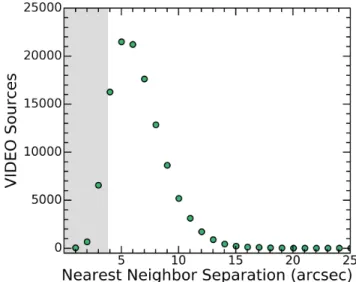
Based on the number distribution of nearest-neighbor source separations of ∆θ_{. 3.}008 (or about twice the angular resolution of the SERVS data) shown in Figure2, we expect at least 17% of the 117,281 sources in the VIDEO-selected input catalog will be blended in the 3.6 and 4.5 µm IRAC data. This is a lower limit since VIDEO sources with larger intrinsic angular sizes will be blended on even larger spatial scales in the original, position-matched SERVS photometric catalogs. The high fraction of VIDEO sources expected to be blended in SERVS is one of the primary motivations for performing forced photometry with The Tractor.

To avoid biasing our output catalog against faint or ex-tremely red objects that are detected only in the IRAC bands and have no ground-based NIR or optical counter-parts, we also created a secondary input catalog of IRAC-selected sources2. For this catalog, we included all detected SERVS sources lacking a counterpart within 100in the origi-nal VIDEO source catalog. We also required a detection in at least one of the two IRAC bands in the SERVS single-band 3.6 and 4.5 µm catalogs3_{. The resulting IRAC-selected input}

catalog contains 8,441 sources.

3.3. Fiducial Band Selection

The Tractor generates a user-defined model of the sur-face brightness profile (see Section 3.4) of a source at a given “fiducial” band with high-spatial-resolution imaging and then convolves this model with the PSF of each remain-ing, lower-resolution band. Thus, the first step in our source modeling procedure is to determine the fiducial band. For the VIDEO-selected catalog, we use the VIDEO Ks-band data

to define the fiducial high-resolution model of each source when possible since this band is closest in wavelength to the IRAC bands. However, for sources in the VIDEO-selected catalog with non-detections at Ks band, we select a fiducial

VIDEO band with a detection and valid flux entry with a preference for the band with the next closest central wave-length to the 3.6 µm IRAC data. We note that, while we could select an optical band from the CFHTLS-D1 data as the fiducial band, this might result in the loss of very red ob-jects from the catalog, and the possible misappropriation of infrared flux to unrelated galaxies with blue optical-infrared colors.

2_{We emphasize that we perform forced photometry using The Tractor on}

both the VIDEO-selected and IRAC-selected input catalogs, thus producing two separate output multi-band source catalogs.

3_{http://irsa.ipac.caltech.edu/data/SPITZER/SERVS/}

Figure 2. Number distribution of nearest-neighbor VIDEO cata-log source separations (∆θ). The grey-shaded portion highlights the population of VIDEO sources with ∆θ < 3.008 that are ex-pected to be blended in the original catalog of SERVS IRAC aper-ture photometry within a radius of 1.009, which corresponds to the FLUX_APER_2_1 and FLUX_APER_2_2 apertures for the 3.6 and 4.5 µm bands, respectively.

We follow a similar strategy for the IRAC-selected catalog of red sources detected in at least one IRAC band that lack a counterpart detected in any of the VIDEO bands in the orig-inal VIDEO catalog. If a source is only detected in a single IRAC band, then that band is the fiducial band. However, if both the 3.6 and 4.5 µm bands are detected, then we select the 3.6 µm band as the fiducial band. The fiducial band se-lected for each source is provided in the Fiducial_Band col-umn (see Table4in the Appendix) of both the VIDEO- and IRAC-selected output catalogs.

3.4. Surface Brightness Profile Modeling

Once the fiducial band has been determined, we extract an image cutout of each source in the input VIDEO-selected catalog from the mosaicked image at each band using the PYTHON wrapper to the MONTAGE4 toolkit (Berriman & Good 2017), which is able to robustly interpret the complex WCS information in the headers of the Spitzer IRAC mo-saics. The resulting image cutouts each have a half-width of 500. This cutout size represents a trade-off between ensuring that the sources in our test field lie well within the cutout ex-tent and excessive computational costs associated with larger cutout sizes. Next, we create a fiducial band model of the tar-get object as well as any neighboring sources in the VIDEO-selected input catalog that are present in the image cutout.

Table 2. Summary of Image Calibration Parameters

Band Survey Sky Noise Sky Level σGaussian wGaussian

(1) (2) (3) (4) (5) (6) Near Infrared [4.5] SERVS 0.003 0.299 [1.0, 1.95] [0.3, 0.7] [3.6] SERVS 0.002 0.099 [1.08, 2.20] [0.37, 0.63] Ks VIDEO 3.114 −0.306 [1.60, 3.09, 10.0] [0.59, 0.27, 0.135] H VIDEO 2.170 −0.226 [1.60, 3.09, 8.64] [0.61, 0.24, 0.15] J VIDEO 1.418 −0.169 [1.59, 2.94, 7.24] [0.63, 0.30, 0.16] Y VIDEO 1.166 −0.147 [1.61, 3.15, 6.51] [0.54, 0.19, 0.27] Z VIDEO 0.613 −0.130 [1.62, 2.76, 4.87, 11.80] [0.5, 0.1, 0.32, 0.08] Optical z0 CFHTLS-D1 0.774 −0.117 [1.56, 2.72, 6.21] [0.73, 0.05, 0.23] i0 CFHTLS-D1 0.330 −0.096 [1.27, 2.13, 4.35, 10.23] [0.37, 0.42, 0.15, 0.06] r0 CFHTLS-D1 0.248 −0.059 [1.37, 2.27, 4.71, 11.45] [0.36, 0.44, 0.16, 0.04] g0 CFHTLS-D1 0.173 −0.031 [1.57, 2.71, 6.17] [0.43, 0.44, 0.14] u0 CFHTLS-D1 0.258 −0.003 [1.66, 2.84, 6.49] [0.45, 0.42, 0.13]

NOTE—Column 1: Observing band or filter name. Column 2: Survey name. Column 3: Sky (rms) noise. The values are given in native image

units (counts for the VIDEO and CFHTLS-D1 images, and MJy sr−1 _{for SERVS). Column 4: Median background sky level. Units are the}

same as in Column 3. Column 5: Standard deviation of each Gaussian component in our composite Gaussian models of the PSF of each band. The mixture of Gaussians described by these models were used during source modeling and to estimate flux uncertainties. We note that for SERVS we only used these Gaussian PSF model parameters to estimate the flux uncertainties (the in-flight, post-cryogenic PSF model images were used instead during the source modeling stage). Column 6: The relative weights of the Gaussian components from Column 5, normalized to sum to 1.0.

Based on the fiducial-band image, the source of inter-est along with neighboring sources within the cutout are modeled as either unresolved (i.e., a point source) or re-solved. For a source to be considered resolved, we re-quire it to have a low probability of being a star in the VIDEO catalog (PSTAR < 0.1) and an estimated radius r> 0.001. The radius is defined as rsource= θmaj×

p

b/a + 0.1, where θmajis the seeing-corrected half-light, semi-major axis

(KSHLCORSMJRADAS for Ksband in the original VIDEO

source catalog), b/a is the axis ratio (semi-minor/semi-major) of an ellipse describing the source extent (determined from the KSELL VIDEO catalog parameter, where b/a = 1 - KSELL), and the constant 0.1 refers to half the pixel size (0.002) the VIDEO bands.

Photometry for resolved sources is then performed twice - once using a deVaucouleurs profile (equivalent to a Ser-sic profile with n = 4) and once using an exponential profile (equivalent to a Sersic profile with n = 1). The resolved pro-file fit resulting in the lowest reduced chi squared (χ2

red) value

after optimization with The Tractor is reported in our final output catalog.

For the IRAC-selected catalog, we extract an image cutout from each band using MONTAGEand create a model of the source and its neighbors. However, since the sources in the IRAC-selected catalog are typically near the SERVS detec-tion limit, we restrict the source surface brightness profile models to be unresolved point-sources.

3.5. Image Calibration Parameters

After the source model at the fiducial band has been de-termined, this model is convolved with the appropriate PSF for each band/instrument. We use a mixture of circular Gaussians with 2-4 components each to model the PSFs for the ground-based VIDEO and CFHTLS-D1 data. For each VIDEO and CFHTLS-D1 band, we select sources that are likely to be stars based on their bright (but unsaturated) fluxes, Gaussian-like radial profiles, and high PSTAR val-ues. We estimate the number of composite Gaussians needed to describe the source as well as the Gaussian σ values and relative weights by visual inspection. Finally, we use these

estimates as initial guesses to obtain least-squares fits to the multi-component Gaussian PSF parameters for each band us-ing The Tractor. These parameters are listed in Table2. For the SERVS data, the large wings and strong diffraction spikes of the PSF from these diffraction-limited, space-based data led to us using the in-flight post-cryogenic IRAC point re-sponse functions (PRFs) described inHora et al.(2012).

We also specify the sky (rms) noise and the median back-ground sky level for each band. These parameters correct for image contamination from sources such as instrument noise and zodiacal light. The sky noise and sky level values used in each band are listed in Table2.

3.6. Optimization

Given a source with the information described above, The Tractorperforms a least-squares fit to the image data to deter-mine the source brightnesses. While in principle all param-eters may be left free to vary (i.e., source positions, shapes, and fluxes), we found that allowing too many parameters to vary caused some fits to yield unphysical results. To avoid these issues, we held all image and calibration parameters fixed during optimization except for the fluxes, which are left free to vary. This type of photometric fitting strategy is sometimes referred to as “forced photometry”5. Exam-ples of the original multi-band images, models, and χ2_maps

for a blended IRAC source and a non-blended, faint IRAC source for which The Tractor has produced improved multi-band photometry compared to the original input catalog is shown in Figures3and4.

Our implementation of The Tractor required the develop-ment of a parallelized PYTHONdriver script. Parallelization was performed using the Multiprocessing PYTHONmodule. A full run of our script for the 117,281 sources with imaging available over 12 bands in our VIDEO-selected input cata-log took approximately 16 hours on a cluster node with 16 cores and 64 GB of memory. Diagnostic images (original sub-image cutout, source model image, and χ2 _{array) may}

be optionally produced, though this significantly increases the run time of our code.

3.7. Output Catalogs

The forced photometry of the VIDEO- and IRAC-selected output catalogs produce multi-band measurements of source fluxes and magnitudes as well as errors. Information on the source position, fiducial band, best-fitting surface brightness

5_{We note that usage of the term “forced photometry” is not consistent}

throughout the literature. In some publications, the term refers to the process of smoothing all images to match the lowest resolution band and then per-forming matched-aperture photometry. Here, our usage of the term follows fromLang et al.(2016b) and describes the process of using prior informa-tion from a high-resoluinforma-tion band to model the flux at the same posiinforma-tion in lower-resolution bands. VIDEO Ks Image Model χ2_red= 0.10 χ2 -5.00 5.00 15.00 25.00 -5.00 5.00 15.00 25.00 -0.50 0.00 0.50 1.00 VIDEO H -5.00 χ2_red= 0.14 5.00 15.00 25.00 -5.00 5.00 15.00 25.00 -0.60 0.00 0.60 1.20 VIDEO J -5.00 χ2_red= 0.16 5.00 15.00 25.00 -5.00 5.00 15.00 25.00 -0.80 0.00 0.80 1.60 VIDEO Y -5.00 χ2_red= 0.14 5.00 15.00 25.00 -5.00 5.00 15.00 25.00 -0.40 0.40 1.20 2.00 VIDEO Z -5.00 χ2_red= 0.18 5.00 15.00 25.00 -5.00 5.00 15.00 25.00 -0.60 0.60 1.80 3.00 CFHTLS-D1 z0 -0.50 χ2_red= 1.76 0.50 1.50 2.50 -0.50 0.50 1.50 2.50 -1.50 1.50 4.50 7.50 CFHTLS-D1 i0 -0.50 χ2_red= 5.19 0.50 1.50 2.50 -0.50 0.50 1.50 2.50 0.00 10.00 20.00 CFHTLS-D1 r0 -0.50 χ2_red= 5.65 0.50 1.50 2.50 -0.50 0.50 1.50 2.50 0.00 8.00 16.00 24.00 CFHTLS-D1 g0 χ2 red= 4.32 -0.50 0.50 1.50 2.50 -0.50 0.50 1.50 2.50 0.00 8.00 16.00 CFHTLS-D1 u0 χ2 red= 1.73 -0.50 0.50 1.50 2.50 -0.50 0.50 1.50 2.50 -3.00 0.00 3.00 6.00 SERVS [3.6] χ2 red= 4.82 0.07 0.10 0.14 0.16 0.07 0.10 0.14 0.16 -6.00 -3.00 0.00 3.00 SERVS [4.5] χ2 red= 2.57 0.27 0.30 0.33 0.36 0.27 0.30 0.33 0.36 -4.00 0.00 4.00

Figure 3. Example of a source that is clearly blended in the SERVS bands but resolved in the fiducial VIDEO band (for this source, Ks

band). The cutout dimensions are 1000× 1000

and the source was modeled using a deVaucouleurs profile. The left column shows the original image, the center column shows the source model con-volved with the PSF of each band, and the right column shows the χ2image and χ2redvalue after fitting with The Tractor. The colorbar

units are in image counts for VIDEO and CFHTLS-D1 and MJy sr−1

VIDEO Ks Image Model χ2_red= 0.12 χ2 -5.00 5.00 15.00 25.00 -5.00 5.00 15.00 25.00 -0.75 -0.25 0.25 0.75 VIDEO H -5.00 χ2_red= 0.12 5.00 15.00 25.00 -5.00 5.00 15.00 25.00 -1.00 -0.50 0.00 0.50 VIDEO J -5.00 χ2_red= 0.14 5.00 15.00 25.00 -5.00 5.00 15.00 25.00 -1.00 -0.50 0.00 0.50 VIDEO Y -5.00 χ2_red= 0.15 5.00 15.00 25.00 -5.00 5.00 15.00 25.00 -1.20 -0.60 0.00 0.60 VIDEO Z -5.00 χ2_red= 0.16 5.00 15.00 25.00 -5.00 5.00 15.00 25.00 -0.90 -0.30 0.30 0.90 CFHTLS-D1 z0 -0.50 χ2_red= 0.79 0.50 1.50 2.50 -0.50 0.50 1.50 2.50 -1.80 -0.60 0.60 1.80 CFHTLS-D1 i0 -0.50 χ2_red= 6.00 0.50 1.50 2.50 -0.50 0.50 1.50 2.50 -4.00 0.00 4.00 CFHTLS-D1 r0 -0.50 χ2_red= 11.01 0.50 1.50 2.50 -0.50 0.50 1.50 2.50 -7.50 -2.50 2.50 7.50 CFHTLS-D1 g0 χ2 red= 18.51 -0.50 0.50 1.50 2.50 -0.50 0.50 1.50 2.50 -9.00 -3.00 3.00 9.00 CFHTLS-D1 u0 χ2 red= 6.46 -0.50 0.50 1.50 2.50 -0.50 0.50 1.50 2.50 -6.00 -2.00 2.00 6.00 SERVS [3.6] χ2 red= 1.27 0.07 0.10 0.14 0.16 0.07 0.10 0.14 0.16 -1.20 0.00 1.20 2.40 SERVS [4.5] χ2 red= 0.86 0.27 0.30 0.33 0.36 0.27 0.30 0.33 0.36 -1.60 0.00 1.60 3.20

Figure 4. Example of our forced photometry procedure for a source with no blending issues that is much fainter than the example shown in Figure3. The cutout dimensions are 1000× 1000

and the source was modeled using a point source model. The left column shows the original image, the center column shows the source model con-volved with the PSF of each band, and the right column shows the χ2image and χ2redvalue after fitting with The Tractor. The colorbar

units are in image counts for VIDEO and CFHTLS-D1 and MJy sr−1

for SERVS.

model, and χ2_red value after fitting with The Tractor is also included in the output catalogs. We provide these catalogs in the online supplementary information, and present additional details on their contents in the appendix.

3.7.1. Saturated Sources

We note that some of the brightest sources in the VIDEO-selected output catalog may be saturated. Thus, we suggest that users wishing to avoid the inclusion of such sources in subsequent analyses utilizing our Tractor VIDEO-selected output catalog consider the binary saturation flag we have provided in the catalog. The saturation flag column identi-fies sources with a high probability of being saturated based on the comparison between The Tractor and original pho-tometry shown in Figure5. For the VIDEO data, sources with magnitudes brighter than 14.0 for Ks and H band, as well as sources brighter than 14.5, 13.6, and 13.8 for the J, Y, and Z bands, respectively, are flagged as saturated. For the CFHTLS-D1 data, sources brighter than 16.3, 15.9, 15.9, 15.1, and 15.7 for the i0, r0, g0, z0, and u0bands, respectively, are flagged. Finally, sources brighter than magnitude 14.0 for the IRAC 3.6 µm band and 13.5 for the IRAC 4.5 µm band are flagged. For further details, we refer readers to Table4in the appendix.

3.8. Caveats

Although our new multi-band photometric catalogs pro-duced using The Tractor offer important advantages over ex-isting catalogs for blended and/or intrinsically faint sources, there are a number of important caveats. We emphasize that improved photometry of blended IRAC sources can only be achieved if the blended objects are well-resolved in the fidu-cial VIDEO band used to generate the source model. For highly complex, extended sources not well-described by a deVaucouleurs or exponential model, the accuracy of our photometry with The Tractor will be reduced. The inclu-sion of additional surface brightness profile models and/or performing fitting with The Tractor over multiple iterations may help address this issue in the future. We note that our strategy assumes that the source surface brightness profile is the same at all 12 NIR and optical bands included in our anal-ysis. In other words, we effectively assume morphological k corrections are small.

Our photometry also does not take into account spa-tial variations in the PSF or sky background level, which could lead to aperture errors that are difficult to correct and poorer flux measurement accuracy for fainter sources, re-spectively. While in principle it would be possible to provide The Tractorwith position-dependent PSF information for all bands based on models generated using the PSFEXsoftware (Bertin 2011), this would increase the computational cost substantially.

Table 3. Median Photometric Offsets

Band NAll ∆MAll NBlended ∆MBlended NNot Blended ∆MNot Blended

(1) (2) (3) (4) (5) (6) (7) Near Infrared 4.5µm 99009 −0.218 15730 −0.155 25683 −0.043 3.6µm 103911 −0.235 15808 −0.175 28657 −0.097 Ks 98811 −0.230 15928 −0.215 23755 −0.111 H 104752 −0.176 17129 −0.154 25598 −0.035 J 106733 −0.006 17473 0.020 26036 0.118 Y 99516 −0.113 15991 −0.081 23390 −0.014 Z 107651 −0.063 17714 −0.013 28601 0.040 Optical z0 104891 −0.138 17286 −0.008 29651 0.233 i0 105392 −0.008 17332 −0.009 29841 0.224 r0 105044 0.006 17256 0.004 29714 0.198 g0 104124 0.020 17093 0.019 29275 0.172 u0 98416 0.051 16081 0.045 26688 0.202

NOTE—Column 1: Observing band or filter name. Column 2: The number of sources with photometric measurements available in both the

original VIDEO-selected input catalog and our new multi-band forced photometric catalog. Column 3: The median difference in magnitude between our new forced photometry with The Tractor and the original catalog photometry. Column 4: The number of sources known to be blended in the SERVS catalog based on the presence of at least one neighboring source within 3.008 in the VIDEO catalog. Column 5: Same as Column 3, except the median magnitude difference is calculated for blended sources only. Column 6: The number of isolated sources lacking neighbors within 3.008 that were modeled as point sources in our forced photometry and are thus not expected to have any blending issues in the SERVS images. Column 7: Same as Column 3, except here the median magnitude difference is calculated for sources that are not expected to be blended.

Although position-dependent astrometric variations can in principle compromise the photometric accuracy of The Trac-tor, the datasets used here do not suffer significantly from such effects. Both VIDEO and CFHTLS-D1 have relative astrometric uncertainties < 0.001 (Jarvis et al. 2013; Gwyn 2012). For the SERVS data, the IRAC Instrument Hand-book6 _{reports that the astrometry is typically accurate to}

∼ 0.00_{2, or about the size of a single pixel in the VIDEO}

sur-vey. Given these relatively small uncertainties, we don’t ex-pect astrometric errors to be a dominant limiting factor in the accuracy of our forced photometry.

4. RESULTS

4.1. VIDEO-Selected Catalog

We find that about 65% of the sources in the VIDEO-selected forced photometry catalog are extended based on the criteria described in Section 3.4, and require

spatially-6_{http://irsa.ipac.caltech.edu/data/SPITZER/docs/irac}

resolved surface brightness profile models. The high frac-tion of extended sources suggests that the number of blended SERVS sources is indeed significantly higher than our lower limit of 17% (see Section 3.2). Of the resolved sources, the majority are best fit by a deVaucouleurs profile (∼61%) rather than an exponential profile (∼39%). The vast major-ity (∼84%) of the sources were modeled using the VIDEO Ks-band data as the fiducial band.

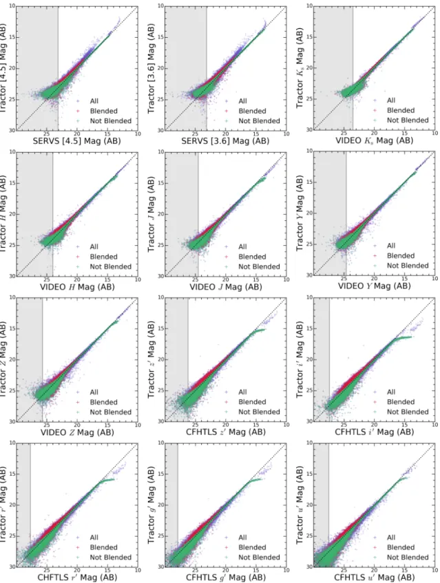
A comparison of the source magnitudes from The Trac-tor forced photometry and the original photometry for the VIDEO-selected catalog is shown in Figure5. Our forced photometry is typically in good agreement with the origi-nal catalog magnitudes, though some scatter is apparent. As expected, the scatter is largest for faint sources. The pho-tometry of these sources is likely more sensitive to noise fluctuations across the image that have not been accounted for by our constant noise assumption. Other factors that may contribute to the scatter include the presence of blended sources, spatial PSF variations, inaccurately matched sources

Figure 5. Comparison between The Tractor and original photometry. For SERVS, we converted the aperture-corrected fluxes measured within

an aperture of radius 1.009 from the original catalog to AB magnitudes. For VIDEO, we show the Petrosian magnitudes. For CFHTLS-D1,

we show the MAG_AUTO magnitudes, which are measured within an elliptical aperture similar to that defined inKron(1980). The dashed

line shows the one-to-one correspondence between The Tractor and original catalog magnitudes. Blended sources in SERVS identified based on the presence of a nearby source in the VIDEO catalog within 3.008 are shown in red. Sources lacking neighbors in VIDEO within 3.008 that were modeled as point sources and, therefore, known to be free of blending issues in SERVS are shown in green. The purple symbols trace all sources. This includes clearly blended/non-blended sources and sources that were modeled with a resolved surface brightness profile. The gray-shaded region highlights the parameter space below the average 5σ detection threshold of each survey.

in the input catalog, and issues with the photometry from the original catalogs. Restricting the comparison to “iso-lated” sources that lack a neighbor within 3.008 in the VIDEO-selected input catalog and were also fit with point source models in the Tractor forced photometry further reduces the scatter in Figure5.

Table 3 summarizes the median difference between our new forced photometry and the original photometry at each band for all sources, blended sources, and isolated point sources (non-blended sources). The magnitudes of the off-sets between The Tractor and original catalogs are dominated by sources at or below the original detection thresholds of the respective surveys, a regime in which accurate source ness measurement is difficult. The uncertainty in the bright-nesses of these faint sources is indicated by their large errors in our output multi-band catalog as well as in the original VIDEO, CFHTLS-D1, and SERVS catalogs.

4.2. IRAC-Selected Catalog

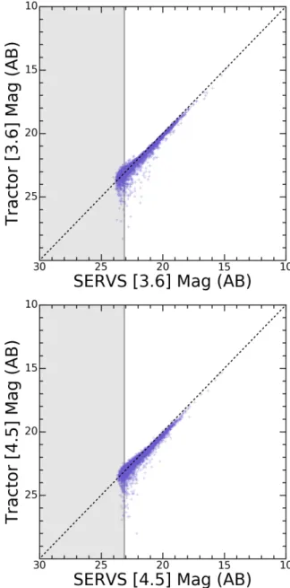
In Figure 6, we compare the SERVS photometry from the IRAC-selected input catalog with the results of our new forced photometry. The photometry in each of these catalogs is generally in good agreement, except for a small population of very faint sources near the SERVS detection limit where the scatter increases notably. These sources may be extended and characterized by inherently low surface brightness emis-sion, making our assumption of a point source surface bright-ness profile inadequate. It is also possible that the original photometry overestimated the source brightness for many of these objects by erroneously including noise and/or emission from nearby confusing sources.

Since the IRAC bands themselves were used as priors, no de-blending was possible. The primary benefit of performing forced photometry on the IRAC-selected catalog is the abil-ity to identify faint VIDEO and CFHTLS-D1 counterparts to extremely red sources only detected previously in the IRAC bands. Of the 8,441 sources in the IRAC-selected input cat-alog7, photometric measurements at Ks-band were possible

using The Tractor for ≈ 69% of the sample. We emphasize that this population of new Ks-band detections represents

in-trinsically faint sources that fall below the detection threshold in the VIDEO single-band catalogs, but can be successfully measured with our forced photometry approach.

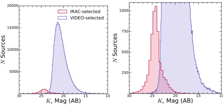
Figure 7 compares the number distribution of Ks-band

source magnitudes from the original VIDEO-selected in-put catalog with measurements from our new IRAC-selected forced photometric catalog. The distribution of new Ks-band

source magnitudes clearly demonstrates that our forced pho-tometry detects a population of extremely faint, red objects

7_{We refer readers to Section3.2for details on the construction of the}

IRAC-selected input catalog.

Figure 6. Comparison of our new forced photometry and the

IRAC-selected input catalog for the [3.6] (top) and [4.5] (bottom) SERVS bands. We use the original SERVS single-band aperture-corrected catalog photometry measured within an aperture of radius

1.009 and converted to AB magnitudes. The gray-shaded region

highlights the parameter space below the average 5σ detection threshold of the SERVS data. The x- and y-axis data ranges match those from the VIDEO-selected catalog comparison plots shown in Figure5.

that fall below the single-band detection threshold in the orig-inal VIDEO photometry. Such intrinsically faint sources at or slightly below the original image detection thresh-old can only be detected with statistical techniques such as forced photometry that incorporate prior information about the source position from a detection at another band.

10

15

20

25

30

K

s

Mag (AB)

5000

10000

15000

20000

N

S

ou

rc

es

IRAC-selected

VIDEO-selected

10

15

20

25

30

K

s

Mag (AB)

250

500

750

1000

N

S

ou

rc

es

Figure 7. Left: Comparison of the number distribution of Ks-band source magnitudes from the original VIDEO catalog (purple) and our

forced photometry measurements based on the IRAC-selected input catalog (red). The VIDEO-selected histogram represents Petrosian source magnitudes. We emphasize that sources with measurements based on our IRAC-selected forced photometry were not detected in the original

VIDEO catalog. Right: A zoomed-in view of the left panel that highlights the distribution of Ks-band source magnitudes from our new

IRAC-selected forced photometry. 4.3. Depth

In Figures8and9we show the magnitude error8as a func-tion of magnitude for each band of the VIDEO- and IRAC-selected Tractor catalogs. We use these figures to determine the 5σ survey depth for each band by measuring the location in the distribution of magnitudes where the faintest sources reach a magnitude error of 0.2. For the two IRAC bands at 3.6 and 4.5 µm, we find 5σ limits of 23.26 and 23.59 in the VIDEO-selected output catalog, and 5σ limits of 23.26 and 22.86 in the IRAC-selected catalog. Values of the 5σ depths for the remaining bands are provided in Figures8and9. The 5σ depths for our output forced photometry catalogs are gen-erally comparable to the magnitude limits from the original catalogs shown in Table1or slightly deeper.

5. DISCUSSION 5.1. Colors

In Figure 10, we show the 3.6 µm vs. J − Ks colors for

the original VIDEO-selected input catalog (top left panel) and our new forced photometry (top right panel). The same sources are shown in the top left and right panels - the only difference is the photometric catalog used to compute the col-ors. Compared to the top left panel of Figure10, the top right

8_{For a detailed discussion of the calculation of flux and magnitude errors,}

we refer readers to AppendixA.

panel showing the photometry from The Tractor has less scat-ter in the distribution of Lyman break galaxy (LBG)-selected sources (g0− r0 < 1.2 and u0− g0> g0− r0+ 1; Steidel et al.

2002) residing in the redshift range 2.7 < z < 3.3. Figure10

also clearly indicates that the stellar locus at J − Ks≈ −0.2 is

substantially better defined when the source colors are com-puted using The Tractor photometry. This qualitatively sug-gests that the colors, and therefore the underlying photomet-ric measurements, are more robust in our forced photometry catalog compared to the original input catalog. We provide a more quantitative assessment of the improved photometric accuracy of our forced photometry catalog in Section5.2.

In the bottom panel of Figure10, we show the NIR col-ors based on our forced photometry as in the middle panel, but this time we also highlight sources that were not detected in the original catalog. This population of sources that are only identified in our new VIDEO-selected forced photomet-ric catalog has a large degree of scatter, but this is expected given the intrinsically faint nature of many of these objects. We emphasize that some of these sources do in fact lie within the main locus of galaxy colors, but were simply too faint to be detected in the original VIDEO photometry. Thus, for studies geared towards intrinsically faint and potentially rare source populations, our implementation of photometry with The Tractoroffers improved sensitivity compared to tradi-tional positradi-tional matching methods.

15

20

25

30

K

Mag (AB)

0.2

0.4

0.6

0.8

1.0

K

M

ag

E

rro

r (

AB

)

5

σ

= 23

.

88

15

20

25

30

H

Mag (AB)

0.2

0.4

0.6

0.8

1.0

H

M

ag

E

rro

r (

AB

)

5

σ

= 24

.

25

15

20

25

30

J

Mag (AB)

0.2

0.4

0.6

0.8

1.0

J

M

ag

E

rro

r (

AB

)

5

σ

= 24

.

73

15

20

25

30

Y

Mag (AB)

0.2

0.4

0.6

0.8

1.0

Y

M

ag

E

rro

r (

AB

)

5

σ

= 24

.

91

15

20

25

30

Z

Mag (AB)

0.2

0.4

0.6

0.8

1.0

Z

M

ag

E

rro

r (

AB

)

5

σ

= 25

.

61

15

20

25

30

i

Mag (AB)

0.2

0.4

0.6

0.8

1.0

i

M

ag

E

rro

r (

AB

)

5

σ

= 27

.

59

15

20

25

30

r

Mag (AB)

0.2

0.4

0.6

0.8

1.0

r

M

ag

E

rro

r (

AB

)

5

σ

= 27

.

85

15

20

25

30

g

Mag (AB)

0.2

0.4

0.6

0.8

1.0

g

M

ag

E

rro

r (

AB

)

5

σ

= 28

.

24

15

20

25

30

z

Mag (AB)

0.2

0.4

0.6

0.8

1.0

z

M

ag

E

rro

r (

AB

)

5

σ

= 26

.

66

15

20

25

30

u

Mag (AB)

0.2

0.4

0.6

0.8

1.0

u

M

ag

E

rro

r (

AB

)

5

σ

= 27

.

15

15

20

25

30

[3.6] Mag (AB)

0.2

0.4

0.6

0.8

1.0

[3.6] Mag Error (AB)

5

σ

= 23

.

26

15

20

25

30

[4.5] Mag (AB)

0.2

0.4

0.6

0.8

1.0

[4.5] Mag Error (AB)

5

σ

= 23

.

59

Figure 8. Source magnitude versus magnitude error for the VIDEO-selected multi-band catalog produced using The Tractor to perform forced photometry. The 5σ magnitude limit corresponds to a magnitude error of 0.2 (horizontal green line). For each band, we identify the faintest source magnitude at the intersection with the 5σ limit (vertical green line). We provide the value of the 5σ detection threshold for each band in the upper left corner of each plot.

5.2. Photometric Redshifts 5.2.1. Distribution

One of the primary motivations for improving the accuracy of the original multi-band photometry is to obtain more ro-bust photometric redshifts. To test whether we have accom-plished this in our test field, we have derived photometric

red-shifts based on the 12 NIR and optical SERVS, VIDEO and CFHTLS-D1 data described in this study using HyperZ ( Bol-zonella et al. 2000). Our galaxy SED template set-up follows that ofPforr et al.(2013), which is based on stellar popula-tion models fromMaraston(2005). A detailed description of our application of SED fitting and subsequent determination

15

20

25

30

K

Mag (AB)

0.2

0.4

0.6

0.8

1.0

K

M

ag

E

rro

r (

AB

)

5

σ

= 24

.

42

15

20

25

30

H

Mag (AB)

0.2

0.4

0.6

0.8

1.0

H

M

ag

E

rro

r (

AB

)

5

σ

= 24

.

81

15

20

25

30

J

Mag (AB)

0.2

0.4

0.6

0.8

1.0

J

M

ag

E

rro

r (

AB

)

5

σ

= 25

.

29

15

20

25

30

Y

Mag (AB)

0.2

0.4

0.6

0.8

1.0

Y

M

ag

E

rro

r (

AB

)

5

σ

= 25

.

51

15

20

25

30

Z

Mag (AB)

0.2

0.4

0.6

0.8

1.0

Z

M

ag

E

rro

r (

AB

)

5

σ

= 26

.

21

15

20

25

30

i

Mag (AB)

0.2

0.4

0.6

0.8

1.0

i

M

ag

E

rro

r (

AB

)

5

σ

= 28

.

15

15

20

25

30

r

Mag (AB)

0.2

0.4

0.6

0.8

1.0

r

M

ag

E

rro

r (

AB

)

5

σ

= 28

.

45

15

20

25

30

g

Mag (AB)

0.2

0.4

0.6

0.8

1.0

g

M

ag

E

rro

r (

AB

)

5

σ

= 28

.

84

15

20

25

30

z

Mag (AB)

0.2

0.4

0.6

0.8

1.0

z

M

ag

E

rro

r (

AB

)

5

σ

= 27

.

21

15

20

25

30

u

Mag (AB)

0.2

0.4

0.6

0.8

1.0

u

M

ag

E

rro

r (

AB

)

5

σ

= 28

.

41

15

20

25

30

[3.6] Mag (AB)

0.2

0.4

0.6

0.8

1.0

[3.6] Mag Error (AB)

5

σ

= 23

.

26

15

20

25

30

[4.5] Mag (AB)

0.2

0.4

0.6

0.8

1.0

[4.5] Mag Error (AB)

5

σ

= 22

.

86

Figure 9. Source magnitude versus magnitude error for the IRAC-selected multi-band catalog produced using The Tractor to perform forced photometry. The 5σ magnitude limit corresponds to a magnitude error of 0.2 (horizontal green line). For each band, we identify the faintest source magnitude at the intersection with the 5σ limit (vertical green line). We provide the value of the 5σ detection threshold for each band in the upper left corner of each plot.

of photometric redshifts will be presented in Pforr et al. (in preparation).

In Figure 11, we show the number distribution of pho-tometric redshifts based on the original position-matched source catalogs and the new catalogs constructed using The Tractor. For each catalog, only sources with accurate (χ2

red≤

3.0) photometric redshifts and measurements in all 12 bands are shown. Both distributions are clearly dominated by lower-redshift sources, in harmony with the high proportion of sources modeled with resolved surface brightness profiles described in Section 4.1 that are typically associated with lower-redshift objects. We note that the predominance of

Figure 10. Top left: Comparison of the SERVS 3.6 µm magnitudes vs. the J − KsVIDEO colors using the original photometry from the

VIDEO-selected input source catalog (Section3.2). Magnitudes are based on Petrosian, MAG_AUTO, and 1.900apertures for VIDEO, CFHTLS-D1,

and SERVS, respectively. All sources with detections in the [3.6], Ks, J, u0, g0, and r0bands (77,809 sources) are shown as gray symbols.

Sources that satisfy the 2.7 < z < 3.3 LBG criteria ofSteidel et al.(2002) are highlighted in magenta. The population of candidate LBG sources that lie on the stellar locus are likely low-redshift interlopers, such as Galactic halo main-sequence stars (e.g., K subdwarfs;Steidel et al. 2003). Top right: Same as the top left panel, except here all magnitudes are based on our new forced photometry. Bottom: Same as the middle panel, except the additional 30,198 sources that only have measurements in our new forced photometry catalog (i.e., those that were upper limits in the original input catalog) are shown in cyan.

lower-redshift sources is not unexpected given that this red-shift range covers the largest volume of our survey. Due to our sensitivity limitations, we only detect the most luminous galaxies in the highest redshift bins.

The comparison between the original and forced photometry-based photometric redshifts shown in this figure is striking. When using the forced photometry source catalog, we obtain

accurate photometric redshifts that incorporate all 12 bands into the SED fitting for over twice as many sources compared to the original position-matched photometry (52,166 vs. 24,273). Furthermore, the number of high-redshift (z > 4.0) photometric redshifts sharply increases as well when the forced photometry is used. Based on the original catalog, only 9 high-redshift sources are identified, though none of

0

1

2

3

4

5

6

z

phot

200

400

600

800

1000

1200

1400

N

Original Photometry

z

phot

N

0

1

2

3

4

5

6

z

phot

500

1000

1500

2000

2500

3000

N

Forced Photometry

z

phot

N

Figure 11. Left: Distribution of photometric redshifts, zphot, calculated using HyperZ based on the original, positional-matched source

catalog in the square degree test region of XMM-LSS. Details on the calculation of the photometric redshifts are provided in Pforr et al. (in preparation). Only the 24,273 sources with measurements available in all 12 bands and accurate (χ2

red. 3.0) photometric redshifts are included.

The inset axis shows the distribution of the 9 sources with high-redshifts in the range 4 < zphot< 6. Right: Same as the left panel, except here

sources with accurate photometric measurements in all 12 bands from our new forced photometric catalog based on The Tractor. Here, a to-tal of 52,166 sources meet the criteria and are shown on the main axis. The inset axis highlights the distribution of 70 sources with high redshifts. these are beyond z = 5. In contrast, we find 70 candidate

high-redshift sources when using our new forced photometry as input to HyperZ, 5 of which lie in the range 5 < z < 6. Thus, a clear advantage of using The Tractor is a substantial increase in the number of sources with robust photometric redshifts and improved sensitivity to faint, potentially high-redshift sources.

5.2.2. Spectroscopic Redshift Comparison

Photometric redshifts from HyperZ based on the original, multi-band, position-matched catalogs and our new forced photometry are compared to high-quality spectroscopic red-shifts9_{from the VIMOS VLT Deep Survey (VVDS;Le Fèvre}

et al. 2013) and the VIMOS Ultra-Deep Survey (VUDS;Le Fèvre et al. 2015) in Figure12. The top left and right panels of this figure show photometric redshifts from the original VIDEO-selected input catalog and our new forced photom-etry, respectively. As expected given the known prevalence of VIDEO sources that are blended in the SERVS photom-etry, Figure 12illustrates that the photometric and spectro-scopic redshifts are much more tightly correlated when the

9_{The VVDS and VUDS magnitude-limited redshift surveys are based on}

multi-slit spectroscopy over the wavelength range 3600. λ . 9350 and include galaxies up to redshift z ∼ 6.7.

photometric redshifts are determined using forced photome-try. Figure12also shows the standard deviation (σ) of the normalized residuals between the spectroscopic and photo-metric redshifts (∆znorm) and the outlier fraction ( foutlier) for

each photometric catalog. These quantities are defined in Equations1and2below:

∆znorm=

zspec− zphot

1 + zspec

(1)

foutlier= |∆znorm| > 0.15. (2)

For the 1,728 sources with accurate photometric redshifts (χ2

red ≤ 3.0), the original and forced photometry catalogs

have σ = 0.23 and σ = 0.08, respectively. This reduction in scatter for the forced photometry is consistent with the im-provement in the foutlier value, which is 6.54% in the

orig-inal photometry and 1.50% in our new photometric cata-log based on The Tractor. To quantify the reduction in ∆znormfor the forced photometric catalog, we perform a

two-sample Kolmogorov-Smirnov test (Feigelson & Babu 2012) on ∆znormfrom the original and Tractor catalogs. This test

yields a probability of p = 5.6 × 10−5 _{that the two samples}

are drawn from the same parent distribution, verifying that the reduction in the scatter for the normalized redshift resid-uals using forced photometry is indeed statistically

signifi-0

1

2

3

4

z

ph

ot

Original Photometry

1

2

3

4

z

spec

4

2

0

2

4

∆

z

no

rm

σ

= 0

.

23

f

= 6

.

54%

Figure 12. Left: Comparison of spectroscopic redshifts from the VIMOS VLT Deep Survey (VVDS;Le Fèvre et al. 2013) and the VIMOS

Ultra Deep Survey (VUDS;Le Fèvre et al. 2015) with photometric redshifts determined from SERVS, VIDEO, and CFHTLS-D1 (Pforr et

al., in preparation). A total of 1,728 sources are shown. Blue sources have spectroscopic redshifts with 95-100% probability of being correct (flags 3 and 13) and red sources have spectroscopic redshifts that are highly certain with virtually 100% probability of being correct (flags 4 and 14). Only sources with accurate (χ2red≤ 3.0) photometric redshifts are included. The lower panel shows the normalized residual, ∆znorm

(Equation1), as a function of spectroscopic redshift. The standard deviation, σ, and the fraction of outliers, foutlier (Equation2), are also

shown. Right: The exact same sources from the left panel are shown, except here the photometric redshifts are calculated using our new forced photometry.

cant. This remarkable improvement is largely driven by the fact that The Tractor photometry provides photometric mea-surements for a larger number of bands included in our study compared to the original photometry based on the position-matched catalogs.

5.3. Future Science Applications

The multi-band forced photometry of the VIDEO-selected input catalog provides a number of improvements over the original position-matched catalog in key areas including source matching accuracy, IRAC source de-blending, and sensitivity to faint sources below the single-band detection threshold in a given survey. We have demonstrated that these improvements to the photometry lead to more accu-rate photometric redshifts, and in the future we plan to use our new forced photometric catalog to accurately measure galaxy masses to study stellar mass assembly out to z ∼ 5. We will also identify quasar candidates over a wide range of redshifts based on their NIR/optical colors (e.g., following

an analysis similar toRichards et al. 2015), taking advantage of our accurate photometry to study the demographics of ob-scured/unobscured quasars in different cosmic epochs. This will allow us to assess the importance of AGN feedback and how it has evolved over the last 12 billion years.

The forced photometry of the IRAC-selected input catalog, which contains sources with IRAC detections in the original SERVS photometry but no counterparts in any of the original VIDEO source catalogs, showed substantial improvement in the number of source detections in the VIDEO and CFHTLS-D1 bands. At Ks-band alone, the source detection fraction

in-creased dramatically from 0% in the original catalogs to 69% after performing forced photometry with The Tractor. This has important implications for the study of extremely red ob-jects (EROs) that are detected in one or more of the SERVS bands but are not detected in any of the original VIDEO pho-tometry. EROs are believed to be extremely dust-enshrouded, high-redshift galaxies with high star formation rates, and rep-resent an evolutionary stage of rapid assembly (e.g.,Yan et al.

2004;Wang et al. 2012). Despite the relevance of these ob-jects to our understanding of galaxy formation and growth, large samples of EROs are currently lacking. A future anal-ysis of the SEDs and photometric redshifts of EROs iden-tified in SERVS and analyzed with our implementation of The Tractor will provide much needed information on the properties and demographics of these objects, and address important galaxy evolution questions such as the fraction of obscured star formation missed by optical surveys.

We plan to expand our forced photometry implementa-tion to the entire XMM-LSS field as well as the remaining four SERVS fields. Given the availability of comparatively deep ground-based NIR and optical data, this will lead to ac-curate photometric redshift measurements over a large sky footprint, allowing us to maximize the scientific return of the SERVS project. In the NIR, new data from the VISTA Extra-galactic Infrared Legacy Survey (VEILS;Hönig et al. 2017) will provide additional deep data in the J and Ksbands.

Deep optical imaging have recently been made publicly available by the Hyper Suprime-Cam Subaru Strategic Pro-gram Data Release 1 (Aihara et al. 2017), which will al-low us to perform forced photometry on the full XMM-LSS field along with the EN1 field later in 2017. The first data release of the Panoramic Survey Telescope and Rapid Re-sponse System (Pan-STARRS) catalog of optical imaging over 5 bands covering 3π steradian was recently made pub-licly available as well (Flewelling et al. 2016). However, to obtain comparable photometric redshift accuracy to that pre-sented in this work for one square degree of the XMM-LSS field, we will require optical imaging of comparable depth to that of CFHTLS-D1 from the Pan-STARRS Medium Deep Survey (Huber & PS1-IPP Team 2015). This survey covers four of the five SERVS fields (XMM-LSS, EN1, Lockman Hole, and CDFS), and is expected to be released later in the year. Deep optical imaging over the full ES1 and CDFS fields has recently been made available as part of the VST Optical Imaging of the CDFS and ES1 Fields (VOICE;Vaccari et al. 2017), and additional optical imaging of these fields (along with the XMM-LSS field) from the full-depth data release of the Dark Energy Survey (DES;Dark Energy Survey Collab-oration et al. 2016) is expected to be made publicly available in 2020.

We will also perform forced photometry on images from the Spitzer DEEPDRILL survey (P.I. Mark Lacy), which will provide post-cryogenic IRAC imaging to µJy depth of the four predefined Deep Drilling Fields (DDFs) for the Large Synoptic Survey Telescope distributed over an area of 38.4 deg2 (1 Gpc3 at z > 2). Science highlights of the DEEP-DRILL survey include the detection of all the > 1011 _M

galaxies out to z ∼ 6 and the identification of ∼ 40 proto-clusters at z > 2, which will provide numerous targets of in-terest for follow-up with JWST. As is the case for SERVS,

the legacy value of DEEPDRILL directly hinges upon the the availability of accurate multi-band photometry. Thus, our application of forced photometry with The Tractor presented here will serve as an essential tool for ensuring the scientific success of both SERVS and DEEPDRILL, and will provide many important new insights into the physics of galaxy for-mation and evolution.

6. SUMMARY

We have provided a description of our parallelized im-plementation of The Tractor to perform forced photometry on 12 NIR and optical bands from SERVS, VIDEO, and CFHTLS-D1 over a square degree of the XMM-LSS field. The VIDEO- and IRAC-selected input catalogs – which have 117,281 and 8,441 sources, respectively – are used to de-fine the fiducial source positions that establish the location at which a given source is modeled in each band. For the VIDEO-selected input catalog, we found that use of The Tractorlead to the following key advantages compared to position-matched multi-band photometry:

1. By modeling the surface brightness profile of each source in a fiducial, high-resolution VIDEO band and performing forced photometry with The Tractor, we were able to de-blend these objects in the SERVS IRAC images and more accurately measure their pho-tometric properties. This naturally lead to more ac-curate source cross-identification, as evidenced by the improved definition of the stellar locus for The Tractor photometry shown in the color-color plot comparison in Figure10. The importance of these improvements is highlighted by our estimated lower limit of 17% for the number of sources that are clearly resolved in the VIDEO images, but blended in the lower-resolution SERVS data.

2. Our application of multi-band forced photometry pro-vided a higher fraction of source detections in each band. This resulted in a factor of two increase in the number of sources with photometric redshift mea-surements with constraints in all of our optical/NIR bands (Figure 11). As a direct consequence of this, we were able to identify a greater number of candi-date high-redshift sources in our square degree test re-gion. While our new forced-photometry-based pho-tometric redshifts identified 70 objects in the redshift range of 5 < z < 6, the position-matched catalogs de-tected none.

3. Based on comparisons between the photometric red-shifts derived from the position-matched and forced photometry catalogs with spectroscopic redshift mea-surements from the literature, we found that The