Absolute localization of mobile robots in forest environments by correlating ground LiDAR to overhead imagery

(1)

Absolute Localization of Mobile Robots in Forest Environments

By Correlating Ground LiDAR to Overhead Imagery

by

Marwan Hussein

B.A.Sc., York University, Toronto, Canada (2007)

Submitted to the Department of Mechanical Engineering and Department of Engineering Systems Division in partial fulfillment of the requirements for the degrees of

Master of Science in Mechanical Engineering

and

Master of Science in Engineering and Management

MAssACHUSEMrS MN E

OF TECHNOLOGY

JUN 2 6 2014

LIBRARIES

at the

MASSACHUSETTS INSTITUTE OF TECHNOLOGY

May 2014

( Massachusetts Institute of Technology 2014. A rights reserved.

Signature redacted

Department of Mechanical EnginL'ering, System Design and Management

Certified by

Certified and Accepted by.

Accepted by.

May 2014

Signature redacted

Dr. Karl Jagnemma Department of Mechanical Engineering Thesi Spervisor

-Signature

redacted

Tatrick Hale ,Jrctor,_SDM *lvs Program

Signature redacted

Dr. David Hardt Chairman, Committee on Graduate Studies Author

(2)

(3)

Absolute Localization of Mobile Robots in Forest Environments By Correlating Ground LiDAR to Overhead Imagery

by

Marwan Hussein

Submitted to the Department of Mechanical Engineering and the Department of Engineering Systems Division on May 2014, in partial fulfillment of the requirements for

the degrees of

Master of Science in Mechanical Engineering

and

Master of Science in Engineering and Management

Abstract

A method for the autonomous geolocation of ground vehicles in forest environments is presented. The method provides an estimate of the global horizontal position of a vehicle strictly based on finding a geometric match between a map of observed tree stems, scanned in 3D by Light Detection and Ranging (LiDAR) sensors onboard the vehicle, to another stem map generated from the structure of tree crowns analyzed from aerial orthoimagery of the forest canopy. Identification of stems from 3D data is achieved by using Support Vector Machine (SVM) classifiers and height above ground filters that separate ground points from vertical stem features. Identifications of stems from overhead imagery is achieved by calculating the centroids of tree crowns extracted using a watershed segmentation algorithm. Matching of the two stem maps is achieved by using a robust Iterative Closest Point (ICP) algorithm that determines the rotation and translation required to align both datasets. The final alignment is used to calculate the absolute location of the vehicle. The localization algorithm has been tested with real-world data and has been able to estimate vehicle geoposition with errors of less than 2.1 m RMS. It is noted that the algorithm's accuracy is currently limited by the accuracy and resolution of the aerial orthoimagery used.

This method can be used in real-time as a complement to the Global Positioning System (GPS) and Simultaneous Localization and Mapping (SLAM) in areas where signal coverage is inadequate due to attenuation by the forest canopy, or due to intentional denied access. The method has two key properties that are significant: i) It does not require a priori knowledge of the area surrounding the robot. ii) Based on estimated vehicle state, it uses the geometry of detected tree stems as the only input to determine horizontal geoposition.

(4)

Thesis supervisor: Dr. Karl lagnemma Title: Principal Investigator

Robotic Mobility Group

Department of Mechanical Engineering Thesis supervisor: Mr. Patrick Hale Title: Director

SDM Fellows Program

Engineering Systems Division

(5)

(6)

Acknowledgements

I would like to thank my research advisor Dr. Karl lagnemma for his guidance and support during the last two years. His pragmatic approach helped me adapt to the daunting experience of transitioning from industry to academia after an almost 5 year gap. He has taught and inspired me in many ways and got me excited about the future of autonomous robotics. He has become a mentor and a good friend. I also would like to thank Mr. Patrick Hale for his advice throughout my studies at MIT. I have never felt away from home thanks to his warm and friendly attitude. My mother Lubna (Halawa!),

my sister Leen, my brother Sinan and my aunt Ghada can't be thanked enough for their encouragement, love and support during the time in which this research was performed.

This research was supported by the U.S. Army Engineer Research and Development Center (ERDC) under contract number W912HZ-12-C-0027. The contract was monitored by Mr. Matthew Renner who I also thank for providing feedback and ideas throughout the project. Other financial support to the author was provided in the form of scholarships and grants from the National Sciences and Engineering Research Council of Canada (NSERC) known as the Alexander Graham Bell Canada postgraduate scholarship and the NSERC postgraduate scholarship.

At the time of writing of this thesis the consumer electronics market is ripe for yet another wave of disruption. Wearable computers and virtual reality devices are starting to appear in the market, albeit at ridiculously low technology readiness levels. After a lot of time spent thinking, interviewing, and choosing, I have decided to join a quirky little company where we plan to change the face of the computer industry as we now know it. I realize this is going to be a challenging endeavor given the size of the incumbents and the complexity of the technology. Nevertheless, I'm willing to take my chances. As Ralph Emerson once said: "Do not go where the path may lead, go instead where there is no path and leave a trail". This is my calling!

"Per audacia ad astra"

Through Boldness to the Stars Marwan Hussein

Cambridge, Massachusetts, May 2014

(7)

(8)

List of Figures

Figure 1: Horizontal locations of features (7-point stars) as observed by a LiDAR sensor onboard a m obile robot on the ground... 26 Figure 2: Overall thesis development roadmap (Chapters in bold square brackets)... 36 Figure 3: Envisioned operational scenario of a solo mobile robot ... 40 Figure 4: Example of dense coniferous forest during summer season (Harvard

Arboretum, Cambridge, MA, from Google Earth) ... 42 Figure 5: Sensor and mobile robot mission configuration showing the anticipated

m inim um working distances and FOV ... 43 Figure 6: Sequence of operations (flowchart) for localization framework showing the

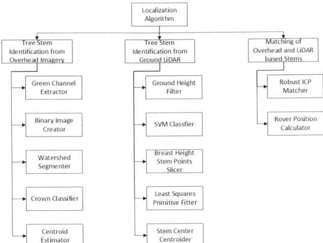
teleoperation and autonomous control scenarios ... 47 Figure 7: Functional breakdown of localization algorithm with three levels of hierarchy:

system , subsystem and com ponents... 50

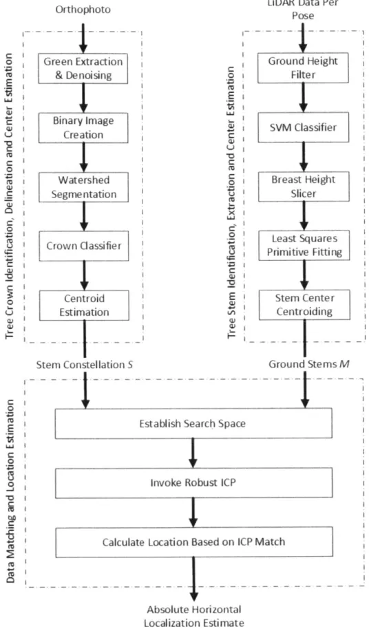
Figure 8: Block diagram of localization algorithm showing the three main subsystems and their com ponents... 52

Figure 9: Optical tree model showing various parameters that define a particular tree ... 57

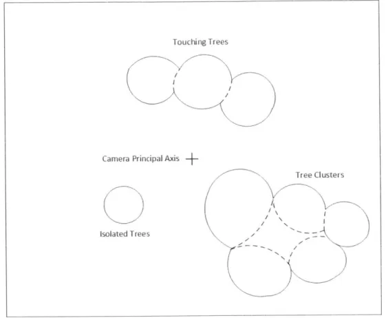
Figure 10: Different morphologies of trees including pyramidal (conifer) trees... 58 Figure 11: Different types of horizontal crown profiles as seen by an overhead camera

showing isolated, touching and clusters of crowns... 60 Figure 12: Image processing flowchart given an input orthophoto image of the

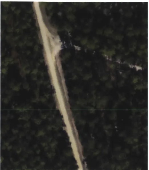
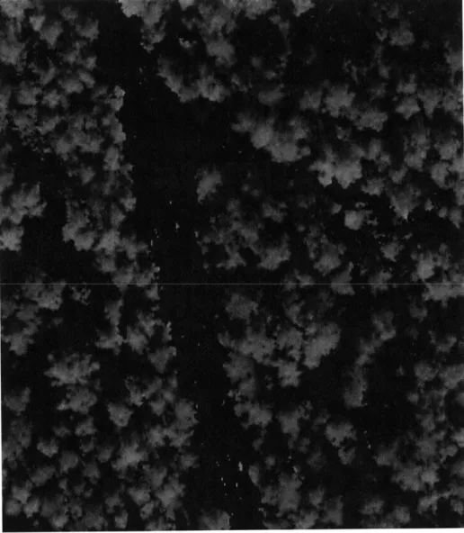
exp lo ration site ... . 62 Figure 13: Original orthophoto input image of Lake Mize test site (Source: USGS

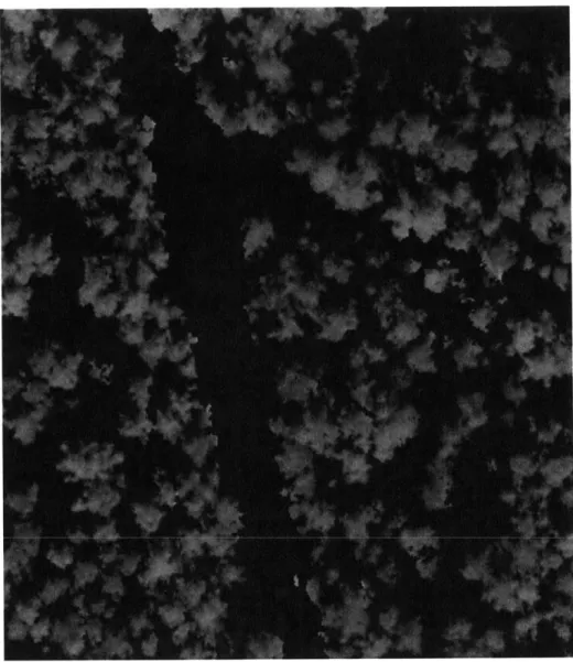
-G oog le E arth )... . 64 Figure 14: Resultant image after green object extraction with all non-green objects

re m o v e d ... 6 5

(12)

Figure 15: Resultant image after application of luminance algorithm that converts RGB to 8 -b it g ray scale ... 6 6

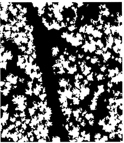
Figure 16: Result after application of Gaussian blur function using erosion and dilation techniques to rem ove spurious pixels ... 67 Figure 17: Resultant image after creating a binary copy of the grayscale image... 68 Figure 18: Result of applying watershed segmentation to binary image N, to delineate

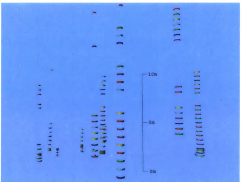
individual tree crow ns... 70 Figure 19: Result after applying the two-stage classifier with green objects denoting valid crowns and red objects denoting invalid crowns ... 71 Figure 20: Final result showing constellation map S with all crowns delineated and valid

centroids denoted by (+) ... 72 Figure 21: Nearest neighbor search results from comparing stem locations in overhead

image to those manually estimated from ground LiDAR data ... 74 Figure 22: Comparison between stems centers detected in overhead image to

hand-labeled stem centers observed in ground LiDAR data... 75 Figure 23: 3D slices of different tree stems for a tree stand observed in 3D LiDAR point

c lo u d [5 9 ] ... 7 9

Figure 24: Centroid calculation by fitting a cylinder primitive [60] ... 79

Figure 25: Data processing flowchart for the stem center estimation algorithm given an input LiDAR dataset of the area surrounding the mobile robot... 80 Figure 26: Sample data showing LiDAR scans of forest grounds at the Lake Mize test site with vertical height color-coding (red: high, blue: low)... 82

Figure 27: Example of a LiDAR dataset at a particular pose showing the simulated

m obile robot, tree stem s and underbrush ... 82 Figure 28: Cartesian space tessellated into 0.5 m x 0.5 m cells [60]... 83 Figure 29: Consecutive LiDAR scans and corresponding stem slices [60]... 85 Figure 30: Example showing cylinder primitive fitment to a single slice of LiDAR data of

a tree stem [6 0 ]... 8 6

(13)

Figure 31: An example of a bad fit showing a large ratio of R to r [60] ... 87 Figure 32: An example of a bad fit showing a large ratio of D to d [60] ... 87 Figure 33: Cylinder placement with respect to the LiDAR sensor with 5 correct cylinder

placements and one wrong (top left corner) [60]... 88 Figure 34: Manually placed markers by hand to identify true stems in ground LiDAR data of the L ake M ize site... . 89 Figure 35: Comparison between the locations of stem centers hand labeled (red) to those

identified automatically by the stem center estimation algorithm (blue) given LiDAR data of Lake Mize site as input. Simulated robot path is shown in pink ... 90 Figure 36: Matching scheme between local maps M and Mi to global map S by finding

the rotation and translation param eters ... 94 Figure 37: SAD correlation process using an input local map and a constellation map [63] ... 9 5

Figure 38: An example of the performance of GMM ICP using two datasets (red and blue) that include outliers and jitter [68]... 96 Figure 39: Data matching flowchart showing the major data processing steps... 97 Figure 40: ICP involves search space positioning based on last known robot geolocation

and systematic search that is comprised of linear and angular stepping... 98 Figure 41: Result from running standard ICP showing skewed position estimate due

presence of one outlier injected to m ap M ... 104

Figure 42: Result from running robust ICP with the same datasets where the outlier was automatically identified by the algorithm and removed ... 104 Figure 43: Geographical area of the test site at Lake Mize, FL, USA (Source: Google

E a rth )... 10 8 Figure 44: Lake Mize test site dimensions and simulated rover path (Image source:

U S G S ) ... 10 8

Figure 45: Simulated mobile robot path in red along with all stem centers identified by

the stem identification and center estimation algorithm... 111

(14)

Figure 46: Geoposition results for path 1 comparing true mobile robot position to

estim ates by the localization algorithm ... 113 Figure 47: Histogram of position error results as provided by the localization algorithm

fo r p a th I ... 1 13 Figure 48: Geoposition results for path 2 comparing true mobile robot position to

estim ates by the localization algorithm ... 1 14 Figure 49: Histogram of position error results as provided by the localization algorithm

fo r p a th 2 ... 1 14

Figure 50: Geoposition results for path 3 comparing true mobile robot position to

estimates by the localization algorithm...1 15

Figure 51: Histogram of position error results as provided by the localization algorithm fo r p ath 3 ... 11 5

fo r p ath 4 ... 1 16

estimates by the localization algorithm... 117 Figure 55: Histogram of position error results as provided by the localization algorithm

fo r p ath 5 ... 1 17

estimates by the localization algorithm...1 18 Figure 57: Histogram of position error results as provided by the localization algorithm

fo r p ath 6 ... 1 18

fo r p a th 7 ... 1 19

estim ates by the localization algorithm ... 120

(15)

Figure 61: Histogram of position error results as provided by the localization algorithm fo r p ath 8 ... 12 0 Figure 62: Geoposition results for path 9 comparing true mobile robot position to

estim ates by the localization algorithm ... 121 Figure 63: Histogram of position error results as provided by the localization algorithm

fo r p ath 9 ... 12 1 Figure 64: Geoposition results for path 10 comparing true mobile robot position to

estim ates by the localization algorithm ... 122 Figure 65: Histogram of position error results as provided by the localization algorithm

fo r p a th 10 ... 12 2 Figure 66: Position error results including mean error, standard deviation and RMSF

produced by localization algorithm for all paths 1-10 ... 124 Figure 67: 2 parameter DOE results versus estimated position error (RMSE) for path 1

d ata (can o n ical case)... 12 5 Figure 68: Impact of number of detected stems per pose on RMSE for path I (canonical

c a se ) ... 12 6 Figure 69: Impact of minimum stem radius on RMSE for path I (canonical case)... 126 Figure 70: Unfiltered geoposition estimates by the localization algorithm for path 1 data

(ICP in blue) as compared to the filtered version using a DKF (KF in green) and the true position data (G PS in red)... 127

(16)

List of Tables

Table 1: Description of functional components of localization algorithm... 50 Table 2: Descriptions of system level inputs and outputs of the localization algorithm.. 53 Table 3: C row n C lassifier Features... 71 Table 4: DOE parameter space with 6 variables and ranges for each ... 73 Table 5: Eight neighborhood classification features for tessellated data... 83 Table 6: A robust algorithm for point-to-point matching of tree center maps in presence

o f o u tlie rs ... 10 1 Table 7: Properties of input data (3 aerial images and one LiDAR point cloud)... 109 Table 8: Input parameters to localization algorithm and simulation program... I11 Table 9: Accuracy results of localization algorithm for all test runs 1-10... 123

(17)

(18)

Nomenclature

Abbreviations ConOps DEM DKF DOE EEPROM ERDC FOV GMM GN&C GPS GPU GUI ICP IMU INS LiDAR MAV MER NIR NSERC RANSAC RGB RMS RMSE RTK SAD SDP SIFT SLAM SNR SURF SVM UAV Concept of Operations Digital Elevation Model Discrete Kalman Filter Design Of Experiments

Electrically Erasable Programmable Read Only Memory Engineering Research Development Center

Field Of View

Gaussian Mixture Model

Guidance Navigation and Control Global Positioning System

Graphics Processing Unit Graphical User Interface Iterative Closest Point Inertial Measurement Unit Inertial Navigation System Light Detection And Ranging Micro Air Vehicle

Mars Exploration Rover Near Infra Red

National Science and Engineering Research Council RANdom SAmple Consensus

Red Green Blue Root Mean Squared Root Mean Squared Error Real Time Kinematic

Sum of Absolute Differences Swiftest Descending Path

Scale Invariant Feature Translorm Simultaneous Localization And Mapping Signal to Noise Ratio

Speeded Up Robust Features Support Vector Machine Unmanned Aerial Vehicle

(19)

UGV Unmanned Ground Vehicle

USGS _{US Geological Survey}

UTM Universal Transverse Mercator WGS84 World Geodetic System

Symbols

Listed in order of appearance

M XM y M Rv Xr yr S xs Es Rr x y z ch cc Xt Yt bh brh cr gin xin Yin g Page 19 of 140

Local map generated from ground LiDAR data x-coordinate of local map M

y-coordinate of local map M

Mobile robot absolute horizontal location vector Absolute location of rover along Easting

Absolute location of rover along Northing Global map generated from overhead imagery Coordinate of a point in global map S along Easting Coordinate of a point in global map S along Northing Distance error

Rotation matrix Translation vector

x-coordinate of 3D profile of tree crown relative to st y-coordinate of 3D profile of tree crown relative to st z-coordinate of 3D profile of tree crown relative to st( Height of base of crown

Normalized radius of curvature

x-coordinate of apex of tree crown relative to stem ba y-coordinate of apex of tree crown relative to stem ba z-coordinate of apex of tree crown relative to stem ba Base height

Breast height

Radius of crown at base Filtered green image Column index of image Row index of image Green channel Red channel Blue channel

Green contrast threshold

Image following green channel extraction Gaussian Blur Function

em base -m base em base se se se b t N G

(20)

a- Gaussian disk radius

i Column index of Gaussian blur disk

j

Row index of Gaussian blur disk

N, Image following application of Gaussian blur function

Nb Binary image

I Input image

d Euclidean distance transform p Input point in 3D space

q Input point in 3D space

WS Watershed segmentation transform

xi Column address of connected pixel

yi Row address of connected pixel

Ne Immediate neighbor

d Diameter of crown object

e Eccentricity

X, Set of points comprising a stem

R Diameter of cylinder primitive base

r Radius of curvature of stem point cluster

P Lowest point in stem

F Feature

C Centroid

C', Classification cost

OM Frame origin of local map M

Os Frame origin of global map S

XSS Easting coordinate of center of search space

YSS Northing coordinate of center of search space

xOD Distance along Easting measured by odometry

yOD Distance along Northing measured by odometry

Rss Rotation matrix of search space

tSS Translation vector of search space

nySs _{Number of rotation steps in angular search space}

nss Number of linear steps in linear search space

o Angular step

dX Linear step along Easting

dy Linear step along Northing

MGEO Local map in global frame Os

XGEO Absolute Easting coordinates of local map M

yGEO Absolute Northing coordinates of local map M

Xe.o/ Linear correction along Easting

(21)

Yu11 Linear correction along Northing

Xstate State vector of simulated mobile robot

Ps Pose

011(11 Maximum angular search space

iMOXs Maximum number of iterations

diaminin Minimum crown diameter

diammxax Maximum crown diameter 1,, Linear dimension of search space

Sm~in Minimum number of stems per pose

enl, Distance error threshold

x0 True Easting position of mobile robot y" True Northing position of mobile robot

Estimated Easting position of mobile robot Estimated Northing position of mobile robot

Subscripts and Superscripts

(- (ij) entry of a matrix

() ith entry of a vector

Units

Units in this thesis are typically given in the SI-system (systeme international) and are

enclosed in square brackets, e.g. [m/s].

(22)

(23)

Chapter 1 Introduction

The Global Positioning System (GPS) has been extensively utilized for decades to localize ground and airborne vehicles [1]. Vehicles with GPS receivers integrated into their navigation systems and running standalone can localize instantly with sub-meter accuracies [1]. Centimeter accuracy has been achieved using augmentation systems and other online correction methods such as Real-Time Kinematic (RTK) [2]. Mobile robots have utilized GPS extensively for outdoor path planning. Sequential traverse waypoints with respect to a global reference system are programmed into the robot and then used

during motion for course comparison and correction using GPS.

Despite advances in GPS measurement methods that have resulted in drastic improvements to localization accuracies, GPS can be rendered ineffective and hence unusable under different scenarios, mainly:

* Attenuation of signals in forest environments by dense tree canopies for rovers operating on the ground to the point where signals can be hardly received [3]. * Multi-path of GPS signals in cluttered environments such as urban city centers

that result in significant positioning errors [3]. Known as the "urban canyon" effect, facades of tall and large buildings reflect GPS signals multiple times before reaching the robot's receiver, thus increasing pseudoranges and skewing final position estimates.

* Intentional GPS signal spoofing, dithering or denied access could render the service inaccessible and potentially unreliable for continuous and real-time localization purposes [3].

Due to the limitations noted above in the performance and reliability of GPS based navigation, non-GPS based techniques have been utilized for robot geopositioning. Dead reckoning frameworks that do not rely on GPS and use Inertial Measurement Units (IMU) have been used extensively [4]. Based on a known reference position, attitudes and accelerations of the robot in all three axes are integrated over time to produce

(24)

positional estimates in real-time. However, due to the continuous drift in attitude estimation by the IMU, this technique is prone to ever increasing errors in measured position [4]. Such drifts, which theoretically could be unbounded, cause considerable challenges for rovers that need to perform precision operations within close proximity to waypoints of interest.

Non-GPS and non dead-reckoning techniques have been developed over the past few years to address the limitations discussed above. Of note are Simultaneous Localization and Mapping (SLAM) algorithms, which have been successfully utilized to localize rovers in a variety of settings and scenarios [5]. SLAM focuses on building a local map of landmarks as observed by a rover and using it to estimate the rover's local position in an iterative way [5,6]. Landmarks are observed using external sensors that rely on optical (i.e. visible camera or Light Detection and Ranging - LiDAR), radar or sonar based means. Positions of landmarks and that of the rover are estimated a priori

and post priori lbr each pose and then iteratively refined [6]. Position errors could be

initially high but tend to converge as more landmarks are observed and as errors are filtered. Of note are schemes that utilize visual odometry and scan matching whereby successive frames at different poses are matched using least squares methods to determine changes in motion [7]. Although these methods could be computationally expensive, they have been successfully integrated into SLAM to provide real-time position estimation. It is noted that the absolute global location of the starting position of the rover needs to be known in order for subsequent poses to be georeferenced [6].

This thesis builds upon the concept of visual based scan matching by developing a novel vision based algorithm that provides a non-iterative estimate of the global position of a rover. The algorithm estimates robot position by comparing landmarks, in this case tree stems observed on the ground, to tree stems detected in overhead georeferenced imagery of the forest canopy. The method is envisaged to be used in two possible scenarios: i) cooperative robotic exploration scheme whereby airborne images of tree canopy captured by an Unmanned Aerial Vehicle (UAV) are matched to 3D maps of the ground beneath acquired by a LiDAR sensor onboard a rover. ii) Solo robotic exploration scheme whereby 3D maps of the forest are captured by a rover mounted LiDAR sensor and compared to an overhead image library preloaded into the rover a priori. In either scenario, only vision based data products are used to estimate the global position of a rover without reliance on GPS. The proposed scheme is similar in concept to the "kidnaped robot" problem where a robot is required to ascertain its position after being placed in an unknown previously unexplored environment [8]. The presented method is envisaged to be complementary in nature to traditional vision and map based navigation frameworks where it could be invoked on-demand by the rover as the need arises. In essence, we anticipate the algorithm to run in the background at all times as a backup that kicks in whenever the primary GPS localization service is down or becomes unreliable.

(25)

Alternatively, and to enable real-time redundancy in geoposition estimation, the method could be used in tandem with the primary localization service.

1.1 Research Background and Motivation

The work described in this thesis can be categorized under vision based localization and mapping, a field currently garnering lots of attention by roboticists worldwide. In particular, absolute localization without the use of GPS is a new field of

study that is now being investigated. The topic is becoming more important considering the different physical environments (e.g. forests and urban areas), and adversarial conditions such as intentional denied access that make it challenging and sometimes

impossible to operate using GPS.

An interesting problem this thesis seeks out to solve is to investigate what localization methods and/or ways that can be used to circumvent limitations of GPS navigation. With limited access to radio-wave means of localization, inertial techniques are usually considered. However, as mentioned earlier and as will be discussed later in the thesis, inertial navigation is prone to drifts that are unbounded if corrections are not continuously applied. Vision based localization becomes a feasible choice by offering "spoof-proof' localization that only requires exteroceptive sensor inputs from visible light camera and/or LiDAR sensors.

Localization and mapping are two intertwined concepts in the field of vision based navigation. To build a map of its surroundings, a rover uses exteroceptive sensory inputs to construct feature maps composed of the relative locations of objects. To put objects in their respective coordinates accurately, the rover needs to know its location first. To localize, the rover can determine its absolute or relative location based on matching what it observes to what it expects to observe. This presents a "chicken and egg" problem where in order to construct accurate maps of its surroundings; the rover needs to know its location a priori. However, the rover needs to first construct maps of objects around it in order to estimate its location, and vice versa. This particular problem has been the focus of extensive research by the SLAM community and is considered to be outside of the scope of this thesis. The work presented in this thesis is focused on the localization aspect by decoupling it from SLAM and applying novel techniques to determine geoposition through the use of exteroceptive data sources.

Figure 1 illustrates the top-level research problem of the thesis. Any static object detected by a mobile robot on the ground can be used to construct a spatial map composed of the horizontal locations of these objects relative to the robot. Theoretically speaking, at least two features need to be observed in order for the mobile robot to localize itself horizontally. Vertical localization (height) is not considered in this thesis. Relative horizontal locations of objects are typically measured at their centroid for

(26)

symmetric or pseudo symmetric objects such as tree trunks and crowns, or at discrete edges at particular heights for corners of buildings in urban environments.

*

I-Direction of Travel

4

Figure 1: Horizontal locations of features (7-point stars) as observed by a LiDAR sensor onboard a mobile robot on the ground

Using exteroceptive sensor inputs from camera, sonar and LiDAR of the immediate environment, a rover can determine its position by constructing spatial feature maps that can be compared to maps previously collected of the same area. High-resolution orthoimagery of the exploration site provide an excellent ground truth upon which local maps generated by the rover on the ground can be compared against. As illustrated in Figure 1, features detected relative to the rover on the ground will have the same geometric relationship between them regardless of the origin or type of sensor used, given reasonable accuracies. The spatial invariance property of these features is exploited to construct maps that can be compared to preloaded ground truth data of the exploration site. This application of multi-sensor fusion is novel within the context of absolute rover localization.

1.2 Thesis Problem Formulation

1.2.1 Thesis Objectives

The first objective of this thesis is to advance the field of autonomous rover navigation by developing a vision based localization algorithm that relies on

(27)

exteroceptive sensor data to match feature maps collected on the ground to georeferenced ground truth of the exploration site. In other words, given a local feature map constructed

from on board vehicle sensors, M= [(x"AI,yx"f), (x-,V 2),..., (x'',y',)], where xly and y

are horizontal coordinates of features relative to the rover, the algorithm attempts to estimate the rover's absolute horizontal location, R, = [x',y'], by matching M to another feature map S = [(xs s I) 2J)2) s . .-, (s ss7)], where xsi and y S are the absolute

horizontal coordinates of ground truth features observed by other means (e.g. aerial, satellite). Through a least squares approach, the algorithm can generate estimates of the absolute location of the rover depending on the matching result of both datasets. The

theoretical questions to be answered by this thesis are:

1. What kind of features and feature properties can be used to invariantly specify feature locations, within the context of an outdoor environment, as they are detected by the rover on the ground (local map M)?

2. What kind of data, features and feature properties can be used to invariantly specify absolute positions (world coordinates) of features for use as ground truths (global map S)?

3. How to register, in 2D, local maps M to constellation map S while achieving absolute accuracies on the order of the individual accuracies of the data inputs

used E, = [El, E2,..., Ek]? Where E; are the individual metric accuracies of the inputs.

A second objective of the thesis is to demonstrate the efficacy and properties of the localization algorithm in the context of finding the absolute position of a single rover operating in a dense forest environment. In particular, the thesis attempts to answer the following applied questions:

1. What are the specific parameters that mostly affect the localization accuracy, its convergence and repeatability?

2. What is the maximum achievable accuracy performance of the localization algorithm?

3. What are the functional and performance constraints of the localization

algorithm and what are some future steps that can be taken to improve performance, if any?

A third objective of the thesis is to implement the localization algorithm and experimentally demonstrate its ability to provide correct and accurate absolute position estimates using real-world data:

1. Implement the vision based localization algorithm in a common and user-friendly technical computing environment, and thoroughly test it with various real-world sensory datasets of different properties.

(28)

2. Validate the resulting performance data with theoretical estimates given properties of the exteroceptive sensor inputs.

3. Obtain insights on the maximum level of accuracy attainable and expected real-world performance given experimental field data.

Finally, the fourth objective of the thesis is to study and specify typical Concepts of Operations (ConOps) that describe how Unmanned Ground Vehicles (UGV), i.e. rovers, are envisioned to operate using the vision based localization algorithm. In particular, the following are systems questions that will be addressed:

1. What are the important system-level requirements describing the functionality, operability and performance of rover localization in outdoor environments?

2. What is the system architecture and use context envisioned for the localization algorithm? Who are the primary stakeholders, beneficiaries and agents of such a system?

3. What is the optimal envisioned operations concept and how can the algorithm

be integrated into a rover system? What inputs/outputs are expected and what internal processes are employed to provide the anticipated results?

1.2.2 Mathematical Problem Definition

The horizontal map that comprises the global horizontal coordinates of tree stems in aerial imagery is described by:

S = [(x, yr),

(x,

y), ... , (xi, ys)], xs, ys E R

i = 1, 2 ... , m

Where xs; and Vsi are the absolute horizontal coordinates of the centroids (stems) of tree crowns detected in overhead imagery with respect to a worldwide reference frame, e.g. WGS84. mi represents the number of tree stems in the set. The set S can be considered as a constellation of tree crowns, in analogy to star constellations, which can be used for navigation. In this case, tree crowns are used instead of stars for matching purposes.

Local feature maps comprising the relative horizontal coordinates of tree stems detected from onboard LiDAR data can be described by:

M=[(xm, yM), (xM, ym), ... , (xM,, ym")], xm~ym E R

i = 1, 2 ... , n

Where x1; and v";' are horizontal coordinates of tree stems relative to the rover at

each pose. n represents the number of tree stems observed at each pose.

(29)

The localization problem can be described as follows: Given a constellation set S and a relative set M both comprising horizontal locations of stems, how can set M be accurately matched with set S in order to determine the absolute horizontal location of the rover?

Mathematically, the above can be solved using a constrained non-linear optimization scheme such that:

2

arg min Es,GEj2 =

IIRXM

+ t - SI

Such that R > 0, t > 0

Where R and i are the horizontal rotation matrix and translation vector needed to transform M to match S. E is the square of the Euclidean distance error between the transformed M and constellation set S, i.e. the square of the norm of the error vector E. In theory, E should be proportional to ES:

E oc Es, Es = [El, E2 ..., E]

i = 1,2, ... , k

Where k is the number of local sets M, or number of poses, assuming one set M per pose. The transformed set M is then used to retrace the origin of observations for each stem to estimate the absolute location of the rover.

1.2.3 Constraint on Thesis Scope

The scope of this thesis is limited to finding the absolute location of a rover within a constrained search space centered on the best-known position of the rover. This scheme is in contrast to performing a brute force global search that is not limited to a particular geographic area. Considering real-time applications of this algorithm, a global search scheme would not be time efficient, or necessarily accurate enough. The implication of such a constraint would require the algorithm to expect a constant stream of estimated rover poses as determined by its onboard Guidance Navigation and Control (GN&C) system. The algorithm would therefore take horizontal position estimates from the GN&C system, determine the absolute position of the rover using its frameworks and then feed those location estimates post priori to the GN&C system, which in turn employs its own Kalman Filter.

The scenario described above is considered more realistic and is in line with current state-of-the-art in rover navigation and localization.

1.3 Previous Work

This section gives a short overview of the scientific literature relevant to the development and validation of the localization algorithm. The literature search begins

(30)

with reviewing papers on the fundamentals of rover localization using different technologies and techniques. The current state-of-the-art in localization and mapping is discussed along with initial work by other researchers in the field of vision based localization. A specific part of this thesis is based on work performed by past members of the Robotic Mobility Group at MIT specifically in the area of tree stem center estimation

from LiDAR data. Their work is also introduced in this section and described in more detail in the main body of the thesis.

Early terrestrial mobile robot localization techniques employed wheel odometry, inclinometers and compass sensors to determine the robot's position relative to a known starting point [9]. Wheel odometry sensors measure the number of wheel rotations to determine distance traveled while inclinometers measure the direction of the gravity vector relative to the body frame of the vehicle, thus providing a direct measurement of the pitch and roll of the vehicle. A compass is used to measure magnetic heading of the mobile robot with respect to the body frame. Common localization techniques incorporate all of the above measurements as part of a vehicle model and integrate measurements to determine the robot's displacement as a function of time [9,10]. This technique is known as dead reckoning [10]. However, due to wheel slip and azimuthal angle drift in wheel odometers, as well as temperature drifts in inclinometer and magnetic compass readings, errors from dead reckoning increase with time and are theoretically unbounded [10]. For example, during the Mars Exploration Rover (MER) mission, the Opportunity rover wheel odometry sensor once underestimated a 19 m traverse by about 8% [11].

More sophisticated technologies such as Inertial Navigation Systems (INS) have been successfully used to localize rovers with moderate accuracies [12]. Although considered to belong to the class of dead reckoning techniques, INS technology has garnered immense interest during the second half of the last century with many sensors deployed onboard vehicles of all kinds and applications. INS technology typically employs 3-axis gyroscopes integrated with 3-axis accelerometers to form an Inertial Measurement Unit (IMU) [13]. The gyroscope assembly measures vehicle attitude along roll, pitch and yaw with respect to a known body frame, while the accelerometer assembly measures the accelerations along all three axes with respect to a known body frame [13]. To determine location with respect to a starting position, the vehicle's state model comprised of the attitude and acceleration data is integrated over time. This technique still suffers from error drifts that are theoretically unbounded. However, the technique provides much higher accuracy than inclinometers and compasses because of the low drift rate and low noise of the 3-axis gyroscope and the 3-axis accelerometers [13]. Regardless of what sensor technology is used, the starting position of the vehicle needs to be known in order for subsequent data to be referenced.

(31)

The satellite based GPS system has been extensively used for terrestrial navigation and localization applications. GPS technology relies on a satellite constellation that provides global coverage of the earth (US Navstar system) [14]. To localize, a vehicle carrying a GPS receiver requires at least 4 satellites overhead with direct line-of-sight [14]. Each satellite sends a carrier signal with timing information that is decoded by the receiver. By comparing the time when the signal was sent to the time it was received, a receiver can determine the distance traveled through the speed of light relationship. With satellite-to-receiver distance information known, and by using the ephemeris of satellites overhead, a receiver can triangulate its 3D position with accuracy limited to the timing error between the clock on the satellite and that used by the receiver

[15].

Real-time GPS accuracies, with no corrections applied, have been reported on the order of 5 m (spherical) [16]. For higher accuracy applications, techniques such as Differential GPS (D-GPS) are used to attain accuracies at the sub-meter and decimeter level [16]. Since the GPS signal is dithered intentionally for commercial use (C/A mode), non-corrected GPS position readings arc inaccurate. D-GPS relies on using real-time corrections calculated by static stations on the ground, thus the term "differential". To attain cm-level accuracy, raw GPS position measurements are post-processed using the logged corrections [17]. Other techniques such as Real-Time Kinematic (RTK) provide cm-level accuracy by correlating the incoming carrier signal over time. This technique has the advantage of lower ambiguity interval, which is on the order of 19 cm for the L 1 carrier [18].

In general, GPS is considered a universal localization method that is reliable under normal conditions. However, GPS signals can be easily attenuated in forest and urban environments. In particular, dense forest canopies have the potential of completely blocking GPS signals from receivers operating on the ground [19]. In similar fashion, GPS signals in dense urban centers (city centers with dense vertical developments) tend to be either attenuated or bounced around and delayed in a phenomenon known as multi-path [20]. This "urban canyon" effect has been investigated and several solutions were implemented. Of note are solutions that integrate INS and GPS to form full position-orientation sensor systems. For example, systems offered by companies such as Trimble/Applanix and Novatel rely on GPS as long as signal coverage is reliable and automatically switch to INS based positioning whenever GPS becomes unreliable [21]. Although effective, these systems are sophisticated, bulky and expensive. It is noted that the localization accuracy of this method will degrade in an unbounded fashion in scenarios where there are long GPS outages. This is due to the method's reliance on INS dead reckoning.

Techniques that are different from INS and GPS rely on visual-based sensors and algorithms e.g. visual odometry and scan matching. Visual odometry relies primarily on

(32)

passive camera sensors that are integrated into a mobile robot [22]. Cameras acquire successive images of the terrain and other features surrounding the mobile robot. Visual odometry algorithms track features across successive pairs of images to measure variations in the pose of the robot [22]. Features are typically extracted using various image processing algorithms such as Speeded Up Robust Features (SURF) or Scale Invariant Feature Transforms (SIFT) [23,24]. Visual odometry has been extensively used in terrestrial and space based applications e.g. MER and Curiosity rovers on Mars [25]. The algorithm is fully automated and can be operated in real-time at the expense of moderate processing speeds, which may require a dedicated Graphics Processing Unit (GPU) [25]. Although effective lor relative navigation, visual odometry still requires continuous tie-in to known global benchmarks in order to provide global localization measurements. In addition, visual odometry is prone to unbounded error growth due to the dependence of future poses on previous position estimates [26]. Due to these characteristics, visual odometry is also classified as a dead reckoning technique.

Scan matching is another vision based navigation method that relies on matching 3D point cloud data captured by laser scanning sensors onboard a mobile robot [27]. Unlike visual odometry, scan matching typically relies on point-to-point matching algorithms such as Iterative Closest Point (ICP) [27]. Pairs of scans taken at successive poses are provided to ICP to determine the translation and rotation between the frames. After an alignment is found, a change in the location of the robot can be determined. Similar to visual odometry, scan matching requires moderate processing power in real-time and therefore could require a dedicated GPU. By matching successive frames, scan matching is also prone to unbounded errors that grow from frame to frame. The algorithm still requires the absolute starting locations of the mobile robot in order to georeference successive pose estimates. An example is that of Song et al (2012) who employs scan matching to the problem of determining the relative pose of a mobile robot in dense forest environments [28]. Tree trunks scanned by an onboard 3D laser scanner are processed and abstracted to form an occupancy map of trunks observed at a particular pose. Successive pairs of maps are compared and correspondences are determined based on the observed 3D point patterns. Levinson et al (2011) applies scan matching to a driverless car application by utilizing a particle filter that correlates successive pairs of 360' LiDAR scans to estimate the vehicle pose [29]. The algorithm reduces the complexity of LiDAR data by filtering out non-ground points and retain road data. Road lane stripes and other white markers on the road are extracted and used for matching between successive scans at different poses.

A different class of localization methods does not rely on distance traversed (dead reckoning) or timing signals (GPS), but instead matches local maps of the immediate environment around the robot to global maps of the area the robot is exploring. Maps here imply 2D imagery, 3D point clouds or occupancy grids. The techniques most relevant to this description follow the procedure of feature detection, extraction and

(33)

matching. In this process, features are first detected, delineated and extracted from the global and local maps using image-processing techniques. Local feature maps are then matched to global feature maps to find correspondences. Once the correspondences are found, the features are aligned in order to produce an estimate of the location of the mobile robot with respect to a global rieference system.

Various researchers have tackled the problem of global map matching and have developed algorithms specifically for this purpose. Planitz et al (2005) and Mian et al (2005) evaluated several algorithms that automatically determine correspondences between 3D point clouds [30,31]. However, researchers were not restricted to 3D

applications. Mikolajczyk and Schmid (2005) focused on finding feature descriptors in 2D images [32]. Se et al (2005) utilizes a Hough transform method to extract visual landmarks in 2D frames and a RANdom SAmple Consensus (RANSAC) scheme to compare and match landmarks in local frames to a database map. The method is effective but expects the global map to be free of outliers or "false positives" in order for pair-wise alignment and matching to perform reliably [33]. Zhang (1994) examined use of ICP for surface alignments of 3D maps in several formats, e.g. Digital Elevation Model (DEM) and point clouds [34]. Early work by Hayashi and Dean (1989) aimed at extracting, comparing and matching data from robot based laser scanners to a high resolution global DEM. Their pioneering work was interesting but their simulations yielded poor accuracy because of the large difference in resolutions between the local and global maps used

[35]. Stein and Medioni (1995) worked on comparing global aerial maps to local rover

maps by comparing skylines captured by a camera onboard a mobile robot to a satellite based topographic map. This method required an area with dense topographic features such as mountainous landscapes and has resulted in accuracies on the order of a hundred meters [36]. Behar et al (2005) explored using high-resolution aerial images for use as global maps instead of coarse orbital imagery. However, his method still relied on dense topographic features for feature detection, extraction and matching [37].

Ramalingam et al (2010) utilized a similar approach for use in urban canyons where skyline imagery of buildings are processed to extract features such as edges of buildings, which are compared to aerial or satellite maps of the same area [38]. Accuracies of 2 m were achieved but the algorithm has several limitations mainly that skylines of buildings are expected to be close to the camera. Another limitation is the fact that nighttime operation is not possible due to use of visible light cameras. Majdik et al (2013) utilize a similar approach for localizing a Micro Aerial Vehicle (MAV) looking down onto buildings [39]. Features detected in the downward looking image, such as building edges, are compared using a SIFT algorithm to a global feature database extracted from Google Street View. By matching features in the horizontal plane, the vehicle is capable of determining its global horizontal location. Kretzschmar et al (2009)

utilize a similar approach that is augmented with data from open-source photo websites such as Flickr [40]. Carle et al (2010) build upon prior work by utilizing long-range 3D

(34)

laser scanner data from a mobile robot that is compared to preloaded DEMs. The position estimates are enhanced by incorporating visual odometry and sun sensor measurements. Accuracies on the order of 50 m were reported [41]. Although accurate when compared to results from earlier work, the algorithm relies on external sensor data to drastically improve accuracy, which is not an optimal or reliable scheme in uncooperative environments.

A different method is Simultaneous Localization and Mapping (SLAM), which has been successfully utilized to localize rovers in a variety of settings and scenarios [42,43]. SLAM focuses on building a local map of landmarks as observed by a rover to estimate its local position in an iterative way [42]. Landmarks are observed using external sensors that rely on optical (i.e. visible camera or LiDAR), radar or sonar based means. Positions of landmarks and that of the rover are estimated a priori and post priori for each pose and then iteratively refined. Position errors could be initially high but tend to converge as more landmarks are observed and as errors are filtered. SLAM can be integrated into schemes that utilize visual odometry and scan matching to provide real-time position estimation. Although such techniques do not require a priori knowledge of the locations of landmarks or that of the rover, the global location of the starting position of the rover needs to be known in order for subsequent poses to be georeferenced. Iser et al (2010) implements a particular instantiation of a SLAM algorithm to globally localize a rover [441. At each pose, a local map of the surroundings is produced using onboard sensors. Iser's work is sensor agnostic and only requires at a minimum a 2D occupancy map of features. Global localization is achieved by invoking RANSAC to perform coarse matching between local maps and a global map of the area. The difference in this implementation is that Iser implemented RANSAC as part of a SLAM framework where matches between local and global maps are refined iteratively as maps get built.

In summary, previous work has focused on globally localizing mobile robots using a variety of sensors, algorithms and methods. Considering map-based localization methods, the majority of researchers focused on either matching successive data frames to determine changes in pose, or by matching unobscured data observed locally by the mobile robot to global maps of the exploration area. Localizing robots in obscured environments such as dense forest grounds is a problem that has just recently been garnering interest by researchers. Considering a GPS denied environment, map-based localization becomes challenging in forest environments simply because features observed on the ground by the mobile robot may not necessarily be observable in aerial or orbital based imagery. Therefore, standard map-based localization algorithms will be challenged in providing reliable data in uncooperative environments.

The research undertaken in this thesis tackles the specific scenario of localizing a mobile robot in dense forests using vision based sensors and matching methods as discussed in the following sections.

(35)

1.4 Thesis Overview

A thesis roadmap is shown in Figure 2. The purpose of this roadmap is to logically organize the thesis research, which solves the mathematical problem definition given in Section 1.2. The flow diagram in Figure 2 comprises the development of the vision based localization framework. Specific chapters of the thesis addressing particular details of the modules shown in Figure 2 are specified in bold and in square brackets.

The methodology adopted to undertake the research and develop this thesis has followed the flow shown in Figure 2. Initial work comprised defining the operations concept of a mobile robot in a dense forest. In particular, the use context was investigated in order to determine likely scenarios and applications that would utilize vision based

localization. Chapter 2 takes a detailed look at particular mission scenarios that would

make use of vision based localization and how, in particular, a kidnapped robot scenario can be addressed. The work concludes by specifying a set of operations and functional requirements that detail scenarios, operations aspects and performance parameters for mobile robot localization in dense forest environments.

Based on the operations concepts and requirements established, a top-level architecture of the vision based localization framework was defined. The architecture seeks to capture the important functional building blocks required to perform localization of a mobile robot. This includes defining the subsystems (modules) that are to be integrated as part of the overall framework. In addition, inputs and outputs at the top-level of the framework are defined in order to clarify how the framework can be integrated to mobile robots and their Guidance, Navigation and Control (GN&C) systems. Chapter 2 captures the architectural details of the algorithm and provides specific information regarding compatibility of this algorithm to current navigation workflows.

Following the definition of the mission concepts and requirements, detailed design and implementation of the various components and subsystems of the localization framework were considered. Starting with Chapter 3, detailed designs of each of the three important sub-systems of the vision based localization algorithm are given. The chapter tackles the automatic tree crown identification, delineation and extraction task. This subsystem is responsible for estimating tree crown centers, and hence tree stems, from aerial or orbital imagery. Various image processing algorithms are implemented and explained, most notably, the watershed segmentation algorithm that enables unambiguous delineation of tree crowns. The output from this subsystem is a global map (constellation) comprised of the detected tree stems that are used by the matching algorithm.