Accelerated development of photovoltaics by physics-informed machine learning

Accelerated Development of Photovoltaics by

Physics-Informed Machine Learning

by

Juan Felipe Oviedo Perhavec

Submitted to the Department of Mechanical Engineering

in partial fulfillment of the requirements for the degree of

Doctor of Philosophy

at the

MASSACHUSETTS INSTITUTE OF TECHNOLOGY

May 2020

c

○ Massachusetts Institute of Technology 2020. All rights reserved.

Author . . . .

Department of Mechanical Engineering

May 15, 2020

Certified by . . . .

Tonio Buonassisi

Professor of Mechanical Engineering

Thesis Supervisor

Certified by . . . .

John Fisher

Senior Research Scientist of Electrical Engineering and Computer

Science

Thesis Supervisor

Accepted by . . . .

Nicolas Hadjiconstantinou

Professor of Mechanical Engineering, Chairman, Committee on

Graduate Students

Accelerated Development of Photovoltaics by

Physics-Informed Machine Learning

by

Juan Felipe Oviedo Perhavec

Submitted to the Department of Mechanical Engineering on May 15, 2020, in partial fulfillment of the

requirements for the degree of Doctor of Philosophy

Abstract

Terawatt-scale deployment of photovoltaics (PV) is required to mitigate the most severe effects of climate change. Despite sustained growth in PV installations, tech-noeconomic models suggest that further technical advances and cost reduction are required to enable a timely energy transition in the next 10 − 15 years. This lim-ited timeline is incompatible with the historic rate of materials development: solar cell technologies have taken decades to transition from the laboratory to large-scale commercial applications.

Recently, the convergence of high-performance computing, high-throughput ex-perimentation and machine learning has shown great promise to accelerate scientific research. In this context, this thesis proposes and demonstrates a comprehensive methodology for accelerated PV development. Machine learning constitutes a key component of the new framework, effectively reconciling the formerly disjoint aspects of first-principles simulation, experimental fabrication and in-depth characterization. This integration is achieved by judiciously formalizing material science problems, and developing and adapting algorithms according to physical principles. Under this in-terdisciplinary perspective, the physics-informed machine learning approach allows a 3 − 30× acceleration in various aspects of PV development.

This work focuses in two particular areas. The first thrust aims to accelerate the screening and optimization of early-stage PV absorbers. The high-dimensionality of the material space, and the sparsity of experimental information, make early-stage material development challenging. First, I address the structural characterization bottleneck in material screening using deep learning techniques and physics-inspired data augmentation. Then, I develop a physics-constrained Bayesian optimization algorithm to efficiently optimize material compositions, fusing experimentation and density functional theory with stochastic constraints. These advancements lead to the discovery of several promising lead-free perovskites, and a 3× more stable multi-cation lead halide perovskite.

The second thrust aims to accelerate the industrial transition of more mature PV devices. For this purpose, I reformulate the traditional record-efficiency figure of

merit to include probabilistic and manufacturing considerations, allowing industrially-relevant optimization. Then, a scalable physical inference algorithm is developed by a principled combination of Bayesian inference, deep learning and physical models. This inference model efficiently provides physical insights leading to > 3× faster solar cell optimization. Finally, this approach is expanded to solar cell degradation diagnosis. I reduce the characterization time by > 5× using time-series forecasting methods. Then, the scalable inference model is combined with a game-theoretic interpretability algorithm to elucidate physical factors driving degradation.

Together, these methodology and results can dramatically accelerate PV technol-ogy development, and have a timely impact in climate change. The physics-informed models expand the horizon of applied machine learning, and the fundamental ap-proach of this work is applicable to other energy materials and systems, such as thermoelectrics and batteries.

Thesis Supervisor: Tonio Buonassisi Title: Professor of Mechanical Engineering Thesis Supervisor: John Fisher

Acknowledgments

It takes a village to raise a child. Scientific research is not different. This work could not have been possible without the guidance and dedication of a large community of colleagues, family and friends across the world. Words here are exiguous to thank each one of you for your contributions and support.

Of course, I have to start by thanking my academic advisors Prof. Tonio Buonas-sisi and Dr. John Fisher for their outstanding mentoring and guidance, and their intellectual courage of doing interdisciplinary research. Since we met five years ago, Tonio has offered me unmatched vision, support and professional resources around the world, allowing me to have a career and do research in topics I am truly pas-sionate about. Thank you the remarkable collaboration network spanning continents and time zones. As my advisor in machine learning, John has taught me a lot about approaching and solving complex problems, clarity of concepts and communication, intellectual curiosity, and a great sense of humor. I thank both of them for the outstanding intellectual freedom and academic guidance they gave me, and the com-munity they fostered in their respective laboratories. I would also like to thank my committee members, Prof. Rafael Goméz Bombarelli and Prof. Jeehwan Kim, for their great intellectual contributions. I am very fortunate of having such great re-searchers and persons as mentors and colleagues.

In the same way, I am grateful to all my colleagues in the MIT Photovoltaics Labo-ratory, the Sensing Learning and Inference Laboratory at MIT, and the Singapore and MIT Alliance of Research and Technology. I acknowledge the great financial support of the Singapore and MIT Alliance of Research and Technology, the US Department of Energy, the Accelerated Materials Development for Manufacturing Program at A*STAR, and TOTAL SA.

It has been a pleasure and a great learning experience to work with you during my graduate studies. In particular, I would like to thank Danny Zekun Ren at SMART, for years of very enriching collaboration, and teaching me the value of curiosity and kindness to do great scientific research. Also, I would like to thank all the great

mentors I had, including Shijing Sun, Ian Matthews, Ian Marius Peters, Liu Zhe, Riley Brandt, Juan Pablo Correa Baena and Jim Serdy. Your cheerful guidance and advice has been fundamental to me during the crossroads of academic life. I sincerely hope I can be as a good mentor and person as all of you are! I also want to thank all my collaborators and friends in the US and Singapore, specially Sarah, Janak, Rachel, Mallory, Amanda, Isaac, Alex, Titan, Richa, Harry, Thway, Hansong, Erin, Nithin, Jeremy, David H., Chris, Genevieve, Sue, Rujian, Johnson, Jose Dario, Sergio, Jonathan, and many more. It has been truly fun and fulfilling to work and learn from you during my time at MIT.

Beyond the laboratory, I have to thank the amazing community of friends in Boston that had become my home away from home: Francis, John, Mike, Ananta, David, Jared, Tej, Craig, Andrew, Daniel, Lauren, Prerna, Steve, Ben, Saffron, Dev, Fernando. The adventures we had together, your love and unconditional support have given me the strength and happiness to always keep moving. Special thanks as well to all the amazing individuals in the Greater Boston Zen Center.

Of course, my close friends and relatives in Ecuador and around the world have been immensely supportive during this time: Pao, Quinti, Lucho, Jose, Marce, Mar-cos, Hugo, Miguel, Michu, Alejo, Alexis, Cami, Clau, Juani, Abue Nelson, Michelle, Lore, tíos & primos. Thank you for all the courage and the faith, the fun moments together, all the visits to the US, and for being next to me during good and bad times.

As well, I am specially grateful to my mentor and friend in Ecuador Prof. Alfredo Valarezo: this thesis will not have been possible without all the trust and dedication he gave me during my undergrad years.

Next, to my best friend and partner, Thalia: this would not have been possible without you. Thank you for all your love. You are my rock and the lightness of my life. I learn from you everyday.

Last but not least, I am immensely grateful to my family: Edmundo, Adriana and Gabriela. Your example, dedication and love are always with me. Thank you for always nurturing my curiosity and being with me, in good and bad times, despite the

distance and the trails of life. I am who I am because of you. And, of course, thanks to God. Life is a great mystery.

Contents

1 Motivation and Overview 19

1.1 Climate change mitigation . . . 19

1.2 Paradigms of photovoltaics development . . . 21

1.2.1 The Edisonian paradigm . . . 21

1.2.2 Accelerated materials development . . . 23

1.3 Thesis overview . . . 24

2 Considerations for Accelerated PV Development 27 2.1 Physics and economics of solar cells . . . 27

2.1.1 Overview of solar cell physics . . . 27

2.1.2 Technoeconomic metrics for PV . . . 29

2.1.3 Challenges for scalable and advanced PV . . . 30

2.2 Promising PV materials . . . 31

2.2.1 Organic PV . . . 31

2.2.2 Perovskite PV . . . 32

2.3 Relevant machine learning methods . . . 34

2.3.1 Machine learning overview . . . 34

2.3.2 Relevant supervised learning algorithms . . . 36

2.3.3 Bayesian optimization . . . 40

2.4 Foundations of accelerated PV development . . . 41

2.4.1 High-throughput experimentation . . . 42

2.4.2 High-performance computation . . . 43

2.4.4 Challenges and strategies for physics-informed machine learning 47

3 Accelerated Screening of PV Materials 51

3.1 Accelerating perovskites screening . . . 52

3.1.1 High-throughput screening for lead-free perovskites . . . 53

3.2 Automating XRD with machine learning . . . 55

3.2.1 Challenges for high-throughput XRD . . . 55

3.2.2 Supervised machine learning model . . . 57

3.2.3 Physics-informed data augmentation . . . 60

3.2.4 All Convolutional Neural Network . . . 62

3.2.5 Allowing model interpretability . . . 68

3.2.6 Screening results . . . 71

3.3 Toward accelerated structural characterization . . . 73

4 Accelerated Optimization of PV Materials 75 4.1 High-throughput optimization of perovskite stability . . . 76

4.1.1 Composition engineering for stable perovskites . . . 76

4.1.2 High-throughput experimental setup . . . 77

4.1.3 Stability figure-of-merit and experimental loop . . . 78

4.2 Physics-constrained Bayesian optimization . . . 81

4.2.1 Gibbs free energy of mixing . . . 82

4.2.2 Data fusion of DFT and experimental optimization . . . 83

4.2.3 Physics-weighted acquisition function . . . 86

4.3 Experimental results . . . 87

4.3.1 Finding optimal compositions . . . 87

4.3.2 In-depth characterization and scientific conclusions . . . 88

4.4 Conclusion and future algorithms . . . 90

5 Accelerated Optimization of PV Devices 97 5.1 Paradigms of device optimization . . . 98

5.1.2 Data-driven optimization framework . . . 100

5.1.3 Total revenue figure of merit . . . 104

5.1.4 Scalable physical inference and optimization . . . 108

5.2 GaAs: accelerating PV learning rate . . . 109

5.2.1 Experimental and simulation details . . . 111

5.2.2 Bayesian network as surrogate model . . . 111

5.2.3 Learning rate acceleration . . . 115

5.3 Perovskites: closing the gap with industrial manufacturing . . . 117

5.3.1 Experimental and simulation details . . . 117

5.3.2 Total revenue optimization . . . 119

5.3.3 Optimum device parameters . . . 121

6 Accelerated Stability Diagnosis of PV Devices 123 6.1 Data-driven stability framework . . . 124

6.1.1 Forecasting JV degradation . . . 125

6.1.2 Time-resolved physical inference . . . 128

6.1.3 Quantification of degradation driving factors . . . 131

6.2 Case study: O-PV degradation . . . 134

6.2.1 Experimental details . . . 135

6.2.2 Data-driven forecasting and diagnosis . . . 137

6.3 Future developments . . . 140

7 Discussion Conclusions 143 7.1 Toward physics-informed machine learning . . . 144

7.2 Insights for next-generation photovoltaics . . . 147

7.3 Closing remarks . . . 149

A Code 151 B Figures and Models 153 B.1 Simulated solar cell efficiency distributions . . . 153

B.3 Inferred parameters for GaAs . . . 156 B.4 Perovskites case study . . . 156 B.5 Degradation forecasting . . . 158

List of Figures

1-1 Scenarios for growth of PV according to IPCC targets. . . 20 1-2 Timelines for material discovery and development, compared to climate

targets . . . 21 1-3 NREL best research solar cell efficiency chart . . . 22 1-4 Accelerated materials development for photovoltaics. . . 24 2-1 Simplified schematic of solar cell, with electrons (𝑒−) and holes (ℎ+₎

flowing in opposite directions during illumination [1]. . . 28 2-2 Crystalline structure of metal halide perovskites. . . 33 2-3 Two-layer-deep, fully-connected, neural network.Adapted from Wikipedia. 37 2-4 Typical structure of a convolutional neural network.Taken from Wikipedia. 38 2-5 Gaussian process regression, with estimated variance bounds,

com-pared to frequentist methods.Taken from Scikit-learn documentation. 40 2-6 Iterations of Bayesian Optimization to optimize unknown function . . 42 2-7 The three elements of accelerated PV development. . . 43 2-8 A. Single-diode equivalent circuit model of a solar cell, B. JV

charac-teristics of a solar cell.Adapted from Wikipedia. . . 46 3-1 Accelerated screening framework, including streamlined solution

pro-cessing platform. . . 54 3-2 Target compounds for accelerated screening, along with notable

resul-tant compounds after applying the proposed methodology. . . 55 3-3 Schematic of our X-ray diffraction data classification framework, with

3-4 Schematic of the best-performing algorithm, our all convolutional neu-ral network.[2] . . . 59 3-5 Effect of data augmentation in a-CNN for dimensionality and space

group classification . . . 67 3-6 Comparison between CAMs and the proposed average CAMs for

cor-rectly and incorcor-rectly classified samples. . . 70 3-7 Machine learning diagnosis results, according to dimensionality . . . . 72 3-8 Screened alloy series showing non-monotonic trend. . . 73 4-1 High-throughput stability optimization of perovskites by DFT-informed

Bayesian optimization. . . 91 4-2 DFT probabilistic constraint for Bayesian optimization, by weighted

acquisition function. . . 92 4-3 Batch Bayesian optimization rounds for instability index minimization. 93 4-4 In-depth characterization of perovskites degradation within our

com-positional space of interest . . . 94 4-5 Evolution of tolerance factor for optimization, and degradation

mech-anisms identified by our approach. . . 95 5-1 Comparison of R&D paradigm and our data-driven approach. . . 101 5-2 Data-driven framework, and examples efficiency-revenue functions. . . 103 5-3 Representative efficiency distributions, and the related value of the

total revenue figure of merit. . . 107 5-4 GaAs solar cell architecture.[3] . . . 111 5-5 General schematic of Bayesian network for process optimization.[3] . . 112 5-6 Neural network surrogate model descriptors, inferring device

parame-ters from 𝐽 𝑉 i curves.[3] . . . 114 5-7 Inferred device parameters for GaAs solar cell. . . 115 5-8 Efficiency for constant temperature sweep vs optimal growth profile. . 116 5-9 MAPbI3 perovskite solar cell architecture . . . 118

5-11 Mean device parameters for two different optimization objectives . . . 122

6-1 Data-driven stability diagnosis framework . . . 126

6-2 Representative degradation trends for O-PV solar cells. . . 127

6-3 Non-regularized time-resolved parameter inference . . . 130

6-4 Regularized time-resolved parameter inference . . . 131

6-5 Time-resolved power loss. . . 134

6-6 A. Schematics of the acceptor and donor molecules used in the O-PV heterojunction [4], B. O-PV solar cell schematic.Oviedo et al., under preparation. . . 135

6-7 RMSE for forecasted degradation, according to the last training time. 138 6-8 Comparison of JV degradation trends for two annealing conditions . 139 6-9 Time-resolved inference for Sample A. . . 140

6-10 Time-resolved inference for sample B . . . 141

6-11 Power loss attributed to the single-diode model parameters for samples A and B.Oviedo et al., under preparation. . . 142

B-1 Encoder structure, the decoder architecture is the inverse of this archi-tecture. . . 154

B-2 Encoder structure, the decoder architecture is the inverse of this archi-tecture. . . 155

B-3 Distributions of parameters 𝑎𝑖, 𝑏𝑖, 𝑐𝑖 inferred via MCMC. . . 156

B-4 Efficiency distributions, for various combinations of temperatures and process conditions. . . 157

B-5 Sensitivity analysis of 𝑓R. . . 157

B-6 Forecasting of 𝐽 (𝑉, 𝑡) as an independent time-series, and as correlated time-series. . . 158

List of Tables

2.1 Challenges and strategies for physics-informed machine learning (ML). 49 3.1 Results of various ML algorithms used for XRD classification . . . 64 7.1 Challenges and algorithm contributions for physics-informed machine

learning (ML). . . 145 7.2 Challenges and contributions for next-generation photovoltaics (PV). 147 C.1 Samples and corresponding compositions used for dimensionality

clas-sification. . . 159 C.2 Samples and corresponding compositions used for space-group

classifi-cation. . . 162 C.3 164 compounds extracted from ICSD using to simulate XRD powder

Chapter 1

Motivation and Overview

1.1

Climate change mitigation

Anthropogenic climate change constitutes an existential risk for modern society. Since the late 1800s, increasing greenhouse gas emissions have caused approximately 1 ∘C global warming, and have produced drastic effects on fragile ecosystems and vulnera-ble populations, including extreme weather events, disruption in food supply, loss of biodiversity, spreading of tropical disease and social conflict [5]. If current greenhouse emission trends remain unchecked, the Earth is expected to surpass 5∘C of warming by the end of this century, substantially increasing the likelihood and magnitude of catastrophic effects.

Societies and nations can promptly act to mitigate the worst consequences of climate change. For this purpose, the scientific consensus advises to limit warming to up to 2 ∘C [6]. By any point of view, doing so requires massive financial, social and technological action within a limited time frame. One of the core measures is the transition from fossil fuels to renewable energy sources. To achieve this, the Intergovernmental Panel on Climate Change (IPCC) estimates that solar and wind energy have to grow by as much as 10 times by 2030 [7].

In this context, one pertinent question arises: Can photovoltaics installations grow fast enough to mitigate climate change? In recent decades, technological and political advances have allowed widespread adoption of photovoltaics (PV). In

2019, the total installed PV capacity amounted to 663 GW, compared to a baseline of 30 GW in 2010 [8]. Although remarkable, this rate of growth is insufficient: the IPCC climate target requires estimated 7-10 TW of installed capacity by 2030 [9]. Figure 1-1 presents projections of various potential scenarios of PV installation growth compared to the 2030 climate goals, according to a seminal study by my colleagues in the MIT PV Laboratoy [9]. Baseline technology and costs are insufficient to reach 2030 climate targets, and novel advanced photovoltaics are required.

Figure 1-1: IPCC targets for installed PV capacity and projected technoeconomic scenarios until 2030. Reproduced from [9].

Advanced photovoltaics include improved crystalline silicon solar cells architec-tures, along with next-generation thin-films. These include technologies such as perovskites and organic solar cells. These technologies promise lower capital cost, cost-of-system and variable costs, along with potentially higher industrial solar cell efficiencies.

How can we take these promising technologies to market as soon as possible? In this doctoral thesis, I develop accelerated methodologies to answer this question, targeting both early-stage and mature solar cell technologies.

1.2

Paradigms of photovoltaics development

1.2.1

The Edisonian paradigm

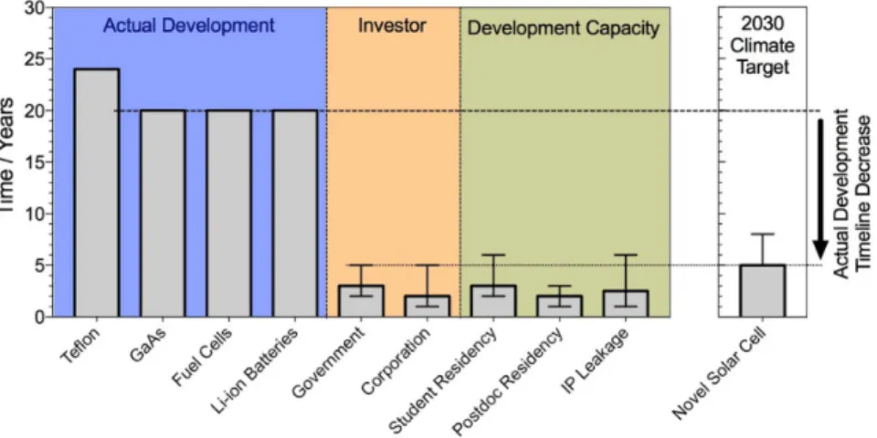
Traditionally, experimental material science has followed the Edisonian paradigm [10, 11]. The paradigm, named after the discovery cycle of the famous inventor Thomas Alva Edison, is based on human intuition, along with combinatorial trial-and-error and slow cycles of in-depth characterization and learning. This paradigm has been dominant in experimental sciences, specially in those in which samples are costly and difficult to make, and underlying theoretical models are insufficient to predict real systems. The Edisonian paradigm has been successful in multiple instances, but it scales poorly to large variable spaces and complex, aggregated systems like solar cells, batteries or transistors. Figure 1-2 contrasts the decade-long timelines for functional material development to the investment, human resources and 2030 climate target timelines [12]. The mismatch among them makes the Edisonian paradigm insufficient to accomplish climate goals.

Figure 1-2: Historic timelines for material discovery and development, along with horizons for research investment, researcher tenure and deployment of PV energy according to 2030 climate targets. Figure reproduced with permission, from [12].

In the case of photovoltaics, the accelerated development challenge has various di-mensions. Advanced PV requires high performance in multiple objectives, including cost, energy conversion efficiency, material abundance and reliability. Furthermore,

solar cell development consists in more than the development of a single material: promising PV absorbers need to be integrated with other materials into functional PV device and module architectures. For instance, due to lengthy characterization and complex physical processes involved, a difficult aspect of modern PV development is achieving high stability (low degradation) under operating conditions. Promis-ing technologies have been used to fabricate solar cells with high efficiency and low manufacturing cost, but limited reliability has inhibited widespread market adoption [13, 14].

Historically, this combinatorial and hierarchical complexity has made solar cell optimization and characterization challenging. One quick look at the National Re-newable Energy Laboratory (NREL) research-solar cell efficiency chart [15], Figure 1-3, illustrates the decade-long efforts to improve solar cell technologies. However, promising technologies, such as perovskite solar cells, which have attractive properties like defect tolerance and simple fabrication methods [13], have shown a substantial rate of improvement in recent years.

1.2.2

Accelerated materials development

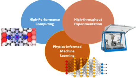
An alternative, emerging paradigm for material development is often referred as ac-celerated materials development or data-driven material development [16, 12]. This paradigm has been popularized in the material science community in the last couple years. The framework combines three emerging technologies:

1. High-throughput experimentation: advances in combinatorial fabrication techniques and laboratory automation have accelerated the rate of fabrication and characterization of new material samples [17, ?, 18].

2. High-performance computing: improved physical models, running in high-performance computing environments have made possible to virtual screen large and complex material parameter spaces. The models include first-principles cal-culations, such as density functional theory or molecular dynamics calcal-culations, and system-level models, such as solar cell or battery simulators [19, ?, 20].

3. Physics-informed machine learning: machine learning techniques, origi-nally developed in fields such as computer vision or nature language processing, have proven useful to inform experimental and computational choices, predict target material properties and find commonalities among material systems. The machine learning models and approaches must be adapted to the material sci-ence domain. [21, 22, 23].

This emerging paradigm has the potential to accelerate the development of high-efficiency, low-cost and reliable PV materials. In photovoltaics, this accelerated de-velopment is manifested in various stages, summarized in Figure 1-4 [12]. First, virtual screening can identify promising materials and inform the experimental pro-cess. Second, high-throughput experimentation and machine learning can accelerated synthesis of PV materials and assembly of PV solar cells. Finally, high-throughput experimentation and machine learning can accelerate the characterization process, and provide insights for automated feedback loops.

Figure 1-4: Accelerated materials development for photovoltaics [12].

1.3

Thesis overview

One of the most challenging aspects of the accelerated development paradigm con-sists in adapting modern machine learning methods to the material science domain. The domain, in contrast to traditional machine learning applications, poses specific challenges due to sparse and scarce data, biased or inaccurate physical models, com-plex computational representations and need of physical interpretability and causal correlation [22, 12, 24, 25].

Motivated by the precedent discussion, this thesis aims to develop and apply physics-informed machine learning methods for accelerated PV and mate-rial development. My proposed methodology aims to be part of a next-generation framework of PV development that successfully addresses imminent climate change and reduces the time-to-market of novel technologies. The accelerated method-ology is applied for three key technoeconomic goals of novel PV: high stability, high manufacturability and scalability. Chapter 2 defines these goals in detail. In particular, the new machine learning techniques aim to increase by 10x the reliability of efficient, promising thin-film PV materials, accelerate 10x the screen-ing of lead-free perovskites, and accelerate device development and characterization by 10–100x. [review]

cells, and explores the challenges and potential solutions for the application of physics-informed machine learning in material science. In subsequent chapters, specific meth-ods are developed and demonstrated for various stages of the PV development cycle: Emerging PV materials: Chapters 3 and 4 focus on emergent PV materi-als for solar cells. In Chapter 3, I develop an automatic machine learning algo-rithm for structural diagnosis, used to accelerate 35× the screening of perovskite and perovskite-inspired materials. This technique aided to report two new promising PV compounds, and 4 compounds synthesized for the first time in film form. In Chapter 4, I propose a data fusion approach for closed-loop optimization of material properties. This technique, in combination with a high-throughput experimentation platform, allowed to identify a 3× more stable multi-cation lead halide perovskite, in comparison to state-of-the-art.

Mature PV devices: Chapters 5 and 6 focus in more mature solar cell tech-nologies, which are already integrated into functional PV devices. Chapter 5 reframes the objective and approach of traditional solar cell optimization to bridge the gap be-tween research and industrial production. Using this new framework, we demonstrate 3× acceleration in the process optimization of full solar cells. Chapter 6 presents a method to accelerate the PV device stability diagnosis, using time series forecasting and physical model interpretability. I demonstrate the approach is able to determine the driving factors of degradation, and is able to forecast the degraded 𝐽 𝑉 with only 10% of the original measurements.

In turn, in Chapter 7 I summarize the main contributions of this work, and outline future pathways and challenges for accelerated materials development.

Chapter 2

Considerations for Accelerated PV

Development

2.1

Physics and economics of solar cells

2.1.1

Overview of solar cell physics

A solar cell is a functional arrangement of various materials that converts sunlight into electricity. The active layer of a solar cell, where charge carriers are generated, is a semiconductor. We define a semiconductor as a material that has an atomic struc-ture with a well-defined set of discrete energy levels, or bands, available to electrons [26]. At 0 𝐾, the valance band corresponds to the energy band that is fully-occupied by electrons. Similarly, the valence band is the lowest energy band with unoccupied states. The energy difference between both bands is the bandgap, 𝐸g. In a

semicon-ductor, at temperatures sufficiently above 0 𝐾, some electrons from the valance band jump to the conduction band. The electron in the conduction band, along with the hole, the unoccupied state in the valance band that can be modeled as a positive-charge particle, allow the material to conduct. In thermodynamic equilibrium, no work can be extracted from the material.

In the case of a solar cell under illumination, photons with energies above 𝐸g

electron-hole pair. This disruption in the equilibrium state creates an electrochemical potential, which translates into net work, or voltage. To produce current and power at a given voltage, the electron and holes need to flow to and be captured at opposite sides of the device. Fig. 2-1 [1] presents an simplified schematic of a solar cell, along with the selective diffusion of holes and electrons into the contacts. In an idealized version, to induce this photocurrent, 𝐽ph, we engineer an energy gradient in the solar

cell by stacking materials of electron or hole selective properties at opposite sides of the absorber layer. In combination with electrical electrodes, this structure compromises a full solar cell.

Figure 2-1: Simplified schematic of solar cell, with electrons (𝑒−) and holes (ℎ+) flowing in opposite directions during illumination [1].

In the same way charge carriers can be excited into the conduction band, they can lose energy and recombine into the valence band. This recombination current 𝐽0,

opposes the photocurrent, and limits the energy that can be extracted from a solar cell. In the context, the diffusion length 𝐿D, the mean distance a carrier can diffuse

in material before recombining, is determined by:

𝐿𝐷 =

√︃ 𝑘𝑇

𝑞 𝜇𝜏 (2.1)

In Eq. 2.1, 𝑘𝑇 /𝑞 corresponds to the thermal voltage constant, 𝜇 is the mobility of minority charge carriers and 𝜏 is the minority charge carrier lifetime. 𝜇 and 𝜏 define the electrical characteristics of a PV material. The accelerated PV material search and optimization of Chapters 3 and Chapter 4 are, in part, motivated by this

figure-of-merit.

Various kinds of recombination losses can occur in the active layer of a PV device, determining an effective bulk lifetime, 𝜏𝑒𝑓 𝑓 for a specific sample or material[26]. This

includes radiative recombination, where an electron-hole emits a photon, Auger recom-bination, where the recombination excites another charge carrier, and trap-assisted recombination, where the defects in the material cause a charge carrier to recombine. Trap-assisted recombination occurring at the surfaces of the device is called surface recombination, and is often described by an inverse lifetime, the surface recombination velocity 𝑆𝑅𝑉 . Finally, other losses are possible, such as carrier collection losses in contacts and optical losses due to non-ideal photon collection. Each solar cell material and architecture presents an specific trade-off between losses and other factors, such as material cost and manufacturing process. In Chapter 5 and Chapter 6, I propose methods for accelerated characterization and curtailment of these loss mechanisms at the device level.

2.1.2

Technoeconomic metrics for PV

Technoeconomic analysis is a powerful tool to explore the cost-performance trade-off of PV energy, and define windows of opportunity for industrial scaling and climate change mitigation. A standard technoeconomic metric to compare different energy sources is the levelized cost of electricity, or 𝐿𝐶𝑂𝐸 [27, 28, 29]. 𝐿𝐶𝑂𝐸 is the ratio between the total lifetime investment on an energy system, and the total energy produced during its lifetime. This ratio defines the break even electricity selling price of a given technology. For PV systems, 𝐿𝐶𝑂𝐸 is calculated by:

𝐿𝐶𝑂𝐸 = 𝐼 + ∑︀𝑁 𝑖=0 𝑂𝑀 (1+𝑟)𝑖 ∑︀𝑁 𝑖=0 𝐸[(1−𝑑)𝑖_] (1+𝑟)𝑖 (2.2)

where 𝐼 is the total initial investment (cost) of the PV system, 𝐸 is the first-year annual energy output of the system, 𝑂𝑀 is the annual operation cost, 𝑑 is the degradation rate, and 𝑟 is a customer-specific discount factor.

energy) technology. The holistic definition of 𝐿𝐶𝑂𝐸 takes into account many factors beyond module cost, including module degradation, variable cost of manufacturing, capital expenditure, energy yield, financing, etc. In this context, the development of novel PV technologies is not a single-objective effort. To become feasible industrial technologies, next-generation PV have to balance multiple technoeconomic require-ments. In the next section, I define these requirements, which will be used as the targets of accelerated PV development in subsequent chapters. In Chapter 5, I pro-pose a novel technoeconomic metric, designed for the transition of PV research to industrial manufacturing.

2.1.3

Challenges for scalable and advanced PV

To satisfy 2030 climate goals, advanced PV requires good performance in various dimensions. These dimensions factor into the 𝐿𝐶𝑂𝐸 of PV, and must be a priority of research and development efforts.

1. High efficiency: high-efficiency solar cells are required to compete with es-tablished technologies. Solar cells below a certain efficiency are not competitive from a 𝐿𝐶𝑂𝐸 perspective [27, 30]. Beyond efficiency, high energy yield under varying spectral and weather conditions is desirable.

2. High manufacturability: Beyond mean or maximum efficiency, the yield and reproducibility of the manufacturing process need to be high, in order to maximize the revenue from a given fabrication batch. Many promises PV technologies struggle in this point, due to complex compositions or sensitive manufacturing processes.

3. High stability: Both the PV material and module lifetimes have to be long enough, under environmental conditions, to be competitive. Many promising PV technologies lack long-term stability.

4. Low cost: Both the variable cost of manufacturing, which scales up with the number of panels produced, (i.e. fabrication cost, labor cost, etc.) and the fixed

capital expenditure (i.e. the cost of building a factory) have to be low [31, 28, 9]. Silicon solar cells tend to have high capital expenditure and manufacturing costs compared to promising technologies.

5. Scalable: New PV requires to use earth-abundant and environmentally friendly materials to justify large scale installations [1, 32].

In this thesis, I focus specially in three of these requirements, as they remain key challenges for novel PV technologies: 1. High manufacturability, 2. High stability, and 3. Scalability. In the next section, I present the two promising PV material classes included in this thesis: perovskites and organic PV.

2.2

Promising PV materials

In the last 15 years, multiple promising PV materials have emerged. However, none of these materials has been competitive with Si and CdTe for large-scale adoption. This thesis focuses in two materials in particular, organic PV and perovskites. However, the proposed methodologies can be extended to the development of any PV material.

2.2.1

Organic PV

One promising thin-film PV technology is organic photovoltaics (O-PV). O-PV de-vices combine semiconducting polymers to create a PV absorber. By modifying the mixing ratio and composition of the polymers, it is possible to tune the optical, elec-trical and physical properties of the polymer blend. Additionally, the solubility of polymers and precursors in organic solvents allows simple and potentially low-cost manufacturing methods, such as spin coating [33].

O-PV materials differ from conventional Si as they are excitonic materials, i.e. the electrons and holes have high binding energy, and are not able to separate as different particles in room temperature. To deal with this challenge, O-PV consist in heterojunction blends of two polymers forming a donor-acceptor interface. The

materials have different ionization potentials and electron affinities, allowing exciton dissociation.

Although O-PV have reached acceptable efficiencies recently, stability is still a no-torious problem. O-PV blends are sensitive to factors such as humidity, temperature and light, and also to interactions with other materials in the solar cell stack [33].

2.2.2

Perovskite PV

An advancement from O-PV is perovskites. In recent years, hybrid organic-inorganic halide perovskites have emerged as a promising thin-film PV technology[13, 34, 35]. The perovskite crystal structure follows the chemical formula ABX3, where the A-ion

corresponds to a single or various organic cations (such as methylammonium CH3NH3,

formamidinium CH(NH)2), the B-ion corresponds to a metal, commonly lead Pb or

tin Sn, and the X-site is a combination of halogens (I, Br, Cl). A schematic of this ideal crystalline structure is presented in Fig. 2-2.

The ideal perovskite structure has cubic symmetry, composed of BC6-octahedra

along cuboctahedral A-cation occupied sites. If the B-ion is large, or the A-ion is small, the tolerance factor of the perovskite decreases below 1, allowing for alterna-tive symmetries such as rhombohedral, orthorhombic and tetragonal. Large A-ions can form layered two-dimensional (2D) or one-dimensional (1D) structures. For the solar cell community, 3D perovskites have shown great promise, and 2D-3D mix-tures have gained recent attention due to increased environmental stability [36, 37]. The illustrated baseline composition, methylammonium lead iodide MAPbI3, and its

variations have demonstrated outstanding diffusion lengths (> 180 𝜇𝑚) and high mi-nority carrier lifetimes (> 300 𝑛𝑠) [38, 39]. A key aspect of lead halide perovskites is defect tolerance. A defect-tolerant semiconductor is characterized by having few ma-terial defects after high-throughput, non-ideal, fabrication conditions, and by limited impact of these defects on lifetime or diffusion lengths. Another important aspect of perovskites is that the bandgap can be tuned for specific application (e.g. multi-junction solar cells). Several variations of this material system are used in this and subsequent chapters.

Figure 2-2: Crystalline structure of metal halide perovskites. (a) Cubic perovskite unit cell. (b) MAPbI3 with octahedral coordination around lead ions. (c)

Cubocta-hedral coordination around the organic ion. Adapted from [13]

In addition to desirable material properties, perovskites are commonly fabricated by solution synthesis. This method is less capital- and energy-intensive than con-ventional semiconductor fabrication methods, requiring high-purity conditions, high temperatures and costly dedicated equipment. This combination of high-throughput fabrication methods and remarkable material properties has allowed a drastic im-provement in perovskite solar cell efficiencies. In the last 5 years, lead halide per-ovskites went from 14% solar cell efficiency to over 22%[15], up to an order of mag-nitude higher rate of development compared to other photovoltaics technologies with various decades in development, such as multi-crystalline silicon or cadmium telluride. The combination of defect tolerance and low-cost fabrication have made perovskites a promising candidate for next-generation industrial solar cells [13].

However, lead halide perovskites have several drawbacks that limit industrial adop-tion. In first place, the best-performing compositions contain abundant Pb+2 lead [40, 32], which has significant biochemical toxicity for humans. Furthermore, lead halide perovskites have poor intrinsic and extrinsic long-term stability. MAPbI is not thermodynamically stable, and mixed-halide and mixed-cation compositions are prone to phase segregation. Even after compositional optimization and encapsulation, perovskites degrade by several efficiency points in the first hundreds or thousands of hours of use [41]. This degradation rate is orders of magnitude higher than commer-cial solar cells, and exacerbates the toxicity drawback mentioned above. Finally, the higher process tolerance and complex compositional space can be counterproductive:

perovskites solar cells present large in-batch variability, increasing the difficulties for industrial adoption. In consequence, determining perovskite compositions and struc-tures that are both defect tolerant, lead-free and stable is major challenge in the field, and a major theme of this work.

2.3

Relevant machine learning methods

In this section, I present various relevant machine learning methods. My aim is not to provide an exhaustive review of the machine learning field, neither to describe in detail specific machine learning algorithms. For this purpose, the reader is invited to consult references [42, 43, 44, 45]. This section provides a basic and intuitive mathematical understanding of core machine learning concepts. These concepts and algorithms are applied, adapted and improved throughout the thesis.

2.3.1

Machine learning overview

Machine learning is a sub-field of artificial intelligence, which focuses on algorithms that can make actions or decisions by learning from past experience, usually referred as "training data". These decision or actions are not explicitly programmed, and are determined by the learning process [43]. To make this learning possible, modern machine learning combines elements of statistics, probability, optimization, program-ming and data mining in a holistic way.

In general, machine learning approaches are categorized as:

Supervised learning

Supervised learning consists in learning a function 𝑔 : 𝑋 → 𝑌 , from a space of possible function 𝐺 referred as the hypothesis space. 𝑔 maps an input space 𝑋 to an output space 𝑌 , based on labeled training data pairs {𝑥𝑖 : 𝑦𝑖}. These labels can be

categorical (classification), continuous (regression) or closed-loop (active learning). Most modern learning models are probabilistic, where 𝑔 becomes a conditional prob-ability 𝑔(𝑥) = 𝑝 (𝑦 | 𝑥), or joint distribution 𝑔 = 𝑝 (𝑥, 𝑦) [43]. Commonly, the learning

process required to choose 𝑔 is formalized as the minimization of a loss function. The loss function 𝐿(𝑦, ˆ𝑦) is an aggregated measure of how well the predictions ℎ𝑎𝑡𝑦 of a certain function 𝑔 fit the training data 𝑦. A loss function we will employ is the negative log likelihood 𝐿(𝑦, ˆ𝑦) = − log 𝑝 (𝑦 | 𝑥) [43]. In general, we are interested in learning 𝑔 with enough generality to perform well in an input space 𝑋′ different from the training dataset. As 𝑔’s of increasing complexity are used, the bias in the training set is reduced at the expense of increased variance in the model training. This fundamental trade-off limits the complexity of 𝑔 and motivates problem-specific model tuning.

There is a wide range of supervised learning algorithms, including linear regression, logistic regression, neural networks, support vector machines, random forests, etc. The next section describes the most relevant supervised machine learning methods used in this thesis.

Unsupervised learning

In contrast to supervised learning, unsupervised learning aims to find structure and representations of an input space 𝑋. This can be interpreted as finding an a priori probability distribution 𝑝𝑋 (𝑥) based on available data 𝑥. Common applications of

unsupervised learning are clustering and dimensionality reduction techniques.

Reinforcement learning

Reinforcement learning is concerned with how an agent interacts with an envi-ronment to maximize cumulative reward. In the absence of labels, the envienvi-ronment response 𝑌 is determined by sequentially taking actions from an action space 𝑆, to maximize some cumulative reward as actions progress. The main focus of reinforce-ment learning is to find an optimal balance of exploration and exploitation than optimizes reward [46]. Bayesian optimization, which is widely utilized in this thesis, can be interpreted as a special case of reinforcement learning.

2.3.2

Relevant supervised learning algorithms

A wide variety of supervised learning algorithms are utilized in this thesis. However, two main techniques are at the core of the methodological and scientific contributions, and are introduced below.

Deep neural networks

Artificial neural networks (ANN) are a machine learning technique loosely inspired by biological neural networks. An ANN is composed of a collection of discrete units, neurons. A neuron takes a series of inputs 𝑋 : [𝑥1, 𝑥2, 𝑥3. . .] and operates on them

according to a series of weights 𝑊 : [𝑤1, 𝑤2, 𝑤3. . .] and a bias 𝑏, such that

∑︀

𝑗𝑤𝑗𝑥𝑗+𝑏.

The output of this operation is then passed through a non-linear function 𝑎 to compute the final output 𝑦. Commonly, the activation function causes the neuron to activate or deactivate according to a certain threshold, such that 𝑎 : R → [0, 1]:

𝑦 = 𝑎 (∑︁

𝑗

𝑤𝑗𝑥𝑗 + 𝑏) (2.3)

Common activation functions are sigmoid, hyperbolic tangent, rectifying linear units (ReLU), etc.

The composition of neurons into layers of input-output connections, forming a deep neural network, greatly expands the model’s capacity [42]. Figure 2-3 shows an schematic of a two layer, fully-connected neural network. Deep neural networks are universal functional approximators, meaning that they can approximate any function. Furthermore, the composition of layers in a deep neural network is an instance of representation learning: neural networks are able to learn a relevant transformation of the input data that maps effectively to the final output. With enough training data, these representations are powerful ways to learn efficient models for high-dimensional problems [42].

Modern deep neural networks are trained by backpropagation [47]. The algorithm computes the gradient of the loss function with respect to the weights of the network for the input-output pairs {𝑥𝑖 : 𝑦𝑖}, and subsequently updates the weights to minimize

Figure 2-3: Two-layer-deep, fully-connected, neural network.Adapted from Wikipedia.

the loss using variants of gradient descent, such as stochastic gradient descent. The chain rule is used to evaluate the loss function gradients along multiple layers, allowing efficient training of large scale networks.

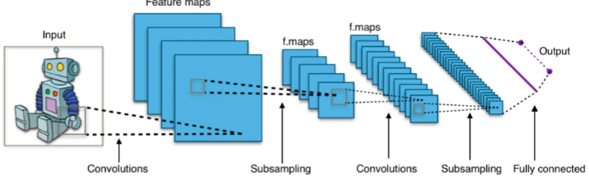
According to neuron and weight connectivity, multiple kinds of neural networks exist, such as convolutional neural networks, recurrent neural networks, etc. For this thesis, an important class is convolutional neural networks (CNNs). CNNs are composed of various hidden layers, in which at least one performs a convolution operation, which is defined as a sliding dot product. In detail, a convolutional kernel, defined by a width 𝑊 , height 𝐻 and input channels 𝐶, is convolved through the input space.

In a fully connected neural layer, each neuron receives an input from every element of the previous layer. In a convolutional layer, neurons receive inputs only from a few neurons in their receptive field. Once the receptive field is defined, the convolution operation allows to share weight and biases among neurons. In this case, for the 𝑗, 𝑘-th hidden neuron, the output is:

𝑎 (︃ _𝑊 ∑︁ 𝑙=0 𝐻 ∑︁ 𝑚=0 𝑤𝑙,𝑚𝑐𝑗+𝑙,𝑘+𝑚+ 𝑏 )︃ (2.4)

Here, 𝑎 is the activation function, 𝑏 and 𝑤𝑙,𝑚 are the values of the shared weight

and bias, and 𝑐𝑥,𝑦 denotes the input activation at position 𝑥, 𝑦.

A final components of CNNs is pooling layers. Pooling, or sub-sampling layers, reduce the input dimensionality by combining the inputs of neurons within an area into a single output. This property allows regularization. Pooling layers can operate in small areas, as local pooling, or as global pooling, in all layers in a neuron.

The use of these three basic ideas: local receptive fields, pooling and shared weights, allow CNNs to be robust to translations (translation equivariance), capture the local structure within an input, and use a reduced number of weights for training [42]. These elements are represented in the CNN schematic of Fig. 2-4.

Figure 2-4: Typical structure of a convolutional neural network.Taken from Wikipedia.

Gaussian process regression

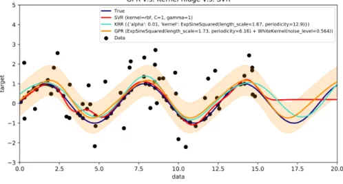
Commonly, supervised learning methods are trained from a maximum likelihood perspective. This approach is useful for prediction and training, however in many scenarios, specially in scientific fields, we require the model to provide a measure of uncertainty. One principled approach, as we will see in later application, is to use Gaussian process regression [44].

Gaussian process (GP) regression assumes a prior over function space that is updated according to training data. Suppose again we have 𝑁 points 𝑥𝑖, 𝑖 = 1, 2, ...𝑁

and labels 𝑦 = 𝑦𝑖, 𝑖 = 1, 2, ...𝑁 ). Given a new input 𝑥*, we are interested in predicting

𝑦* = 𝑓 (𝑥*). If we assume that 𝑓 is a GP, the distribution of the values of 𝑓 at any

assume zero-mean, and then 𝑦* is defined as: ⎛ ⎝ 𝑦 𝑦* ⎞ ⎠∼ 𝑁 (︃ 0, ⎛ ⎝ 𝐾 𝐾𝑇 * 𝐾* 𝐾** ⎞ ⎠ )︃ , (2.5)

where 𝐾 is the covariance matrix for the known inputs, 𝐾* is the covariance

between the new point and the original inputs, and 𝐾**covariance between 𝑦* values.

In the noisy setting, we define the measurements noise as 𝜎.

Then, the probability of 𝑦* conditioned on the given outputs 𝑦𝑖 is given by:

𝑝(𝑦*|𝑦𝑖) ∼ 𝑁 (𝐾*[𝐾 + 𝜎2𝐼]−1, 𝐾**− 𝐾*[𝐾 + 𝜎2𝐼]−1𝐾*𝑇). (2.6)

The conditional distribution allows to estimate uncertainty in unknown regions of the parameter space. The assumption in GP regression, of course, is that output variables close in the input space are highly-correlated. This correlation, which deter-mines in practice the prior over functions, is defined by the kernel function 𝑘(𝑥𝑖, 𝑥𝑗),

𝑘:R𝑛× R𝑛

→ R. Two kernel functions are used in this thesis. The first one is the radial basis function (RBF):

𝑘(𝑥𝑖, 𝑥𝑗) = exp (︂ −𝑙‖𝑥𝑖− 𝑥𝑗‖ 2 2𝜎2 )︂ (2.7) The second kernel, used commonly for Bayesian optimization [48], is the Matérn kernel: 𝑘(𝑥𝑖, 𝑥𝑗) = 𝜎2 21−𝜈 Γ(𝜈) (︁√ 2𝜈 ℎ𝑙)︁ 𝜈 𝐾𝜈 (︁√ 2𝜈 ℎ𝑙)︁ (2.8)

where Γ is the Gamma function, 𝐾𝑣 is the modified Bessel function, ℎ is ‖𝑥𝑖− 𝑥𝑗‖,

𝑙 is the lengthscale, 𝜎 the kernel variance, and 𝜈 is a non-negative parameter, usually a fraction, defining the kernel’s degree of smoothness.

In both cases, the kernel hyper-parameters: lenghtscale, variance, etc. can be inferred by performing maximum likelihood estimation or Bayesian marginalization [?].

other Bayesian models, is that they allow to estimate uncertainty in unknown regions of the variable space, as I will detail in the next section.

Figure 2-5: Gaussian process regression, with estimated variance bounds, compared to frequentist methods.Taken from Scikit-learn documentation.

2.3.3

Bayesian optimization

Multiple problems in material science require the optimization of an blackbox func-tion, i.e. a function that we do not know a priori, but that we can evaluate by an expensive evaluation. This is often the case during experimentation. In this scenario, evaluating a function randomly or based on certain heuristics might not lead to the global optimum, or might not be sample-efficient.

Under these constraints, one principled approach is surrogate-model-based opti-mization, in particular, Bayesian optimization [?, 49, 50].

Bayesian optimization considers the problem of a finding a global optimum (max-imum, or minimum) of an unknown function 𝑓 :

𝑥* = argmax

𝑥 ∈ 𝜒

𝑓 (𝑥) (2.9)

where 𝜒 is a subset of R, or an analogous space. There is no close form for 𝑓 (𝑥), but we can query the function at 𝑥 with noisy evaluations such that E[𝑓 (𝑥)] = 𝑓 (𝑥).

In this setting, Bayesian optimization is a sequential algorithm that, at iteration 𝑛, selects a query location 𝑥𝑛+1, and observes 𝑓 . Based on the observations, it updates

a surrogate model of 𝑓 (𝑥). The algorithm then suggest the next query location according to the expectation and uncertainty of 𝑓 in 𝜒. The algorithm converges when the global optimum 𝑥* has been reached, or when there is no expected improvement according to the surrogate model.

In most implementations, the surrogate model for 𝑓 (𝑥) is a GP regression model, sequentially trained with queried data. The probabilistic nature of the GP allows to define an acquisition function 𝛼(𝑥) : 𝑥 → R so the location of the query 𝑥𝑛+1 is

determined by optimizing an acquisition function 𝛼(𝑥). The acquisition function is designed so it can be optimized easily compared to 𝑓 (𝑥). Intuitively, the optimization of the acquisition functions evaluates the GP posterior uncertainty to guide the op-timization, balancing exploration and exploitation according to the surrogate model. Fig. 2-6 illustrates this procedure.

In this thesis, the acquisition function of interest is expected improvement [45, ?]. Although, it has found to perform greedily in certain problems [51, ?, 52], we found a good empirical performance for our problems of interest, combined with signifi-cant mathematical flexibility for constrained optimization. Expected improvement is defined as: EI(𝑥) = (𝜇𝑛(𝑥) − 𝜏 )Φ (︂ 𝜇𝑛(𝑥) − 𝜏 𝜎𝑛(𝑥) )︂ + 𝜎𝑛(𝑥)𝜑 (︂ 𝜇𝑛(𝑥) − 𝜏 𝜎𝑛(𝑥) )︂ (2.10) where Φ is the standard normal cumulative distribution, 𝜇𝑛 is the mean of the

model’s posterior, 𝜏 is an incumbent target, 𝜎𝑛is the variance of the model’s posterior,

and 𝜑 is the standard normal probability distribution.

2.4

Foundations of accelerated PV development

In this section, I present the fundamental elements of accelerated PV development, summarized in 2-7. Finally, I outline the main challenges of physics-informed machine learning, which constitutes the methodological focus of this thesis.

Figure 2-6: Three iterations of Bayesian optimization, showing the Gaussian process surrogate model and the acquisition function, taken from [50].

2.4.1

High-throughput experimentation

In PV, the emergence of laboratory automation [53, 54, ?, 11] and defect-tolerant PV materials, such as perovskites [34, 13, 32], have increased significantly the through-put of fabrication and characterization processes. Laboratory automation has made possible to accelerate repetitive tasks, and defect-tolerant technologies have reduced the stringent fabrication requirements of silicon or III-V materials.

In general, we can identify the following approaches for high-throughput experi-mentation:

∙ Self-driving laboratories: self-driving laboratories for PV aim for end-to-end automation of the fabrication process, from films to full solar cells. This approach has successfully demonstrated very high throughput recently [55, 56,

Figure 2-7: The three elements of accelerated PV development.

?]. However, the significant degree of process customization and focus in a specific technology / device architecture reduce the flexibility of such setups. ∙ Modular automated laboratories: modular automated laboratories aim to

optimize specific bottlenecks of PV fabrication and characterization. This allows more flexibility than end-to-end automated laboratories, and is the experimental approach we follow in this thesis [57, ?, 58].

∙ Process ergonomics: beyond automation, process ergonomics have significant impact in throughput. Process ergonomics are defined as the acceleration of a process based on the optimization and integration of its various workflows ac-cording to the available resources and other constraints. For instance, choosing a robust and common set of chemical precursors to explore PV material com-positions can have a significant impact on the learning rate and the available exploration space. This approach has been demonstrated in [57], and is also applied in this thesis.

2.4.2

High-performance computation

In this thesis, two classes of PV physical simulation are relevant:

The electronic structure of a semiconductor can be modelled by the many-electron time-independent Schrödinger equation, under the Born-Oppenheimer approximation of fixed charged nuclei. A stationary electronic state is then described by a wave-function Ψ( ⃗𝑟1, ..., ⃗𝑟𝑛) satisfying: [︃ _𝑁 ∑︁ 𝑖 (︂ − ~ 2 2𝑚𝑖 ∇2 𝑖 )︂ + 𝑁 ∑︁ 𝑖 𝑉 (⃗𝑟𝑖) + 𝑁 ∑︁ 𝑖<𝑗 𝑈 (⃗𝑟𝑖, ⃗𝑟𝑗) ]︃ Ψ = 𝐸Ψ (2.11)

where 𝑁 is the number of electrons in the system, 𝐸 is the total ground-state energy, 𝑉 is the potential energy due to the charged nuclei, and 𝑈 is the electron-to-electron interaction energy. In general, Eq. 2.4.2 is not analytically tractable, and for 𝑁 over a few electrons, it quickly becomes numerically intractable.

To deal with these challenges, [59] demonstrated that the probability density as-sociated with the wave-function is able to determine the system. In consequence, solving for the charge density allows to compute all ground-state physical properties in a tractable way, allowing to extract a multitude of properties such as the total energy of the system, the enthalpy of formation of a given compound, the bandgap, etc. In this case, the ground-state energy 𝐸 of the system is written as a functional of the electron density (DFT):

𝐸 = 𝐹 [𝑛(𝑟)] = 𝑇𝑠[𝑛(𝑟)] + 1 2 ∫︁ _{𝑛(⃗𝑟)𝑛(⃗𝑟}′₎ | ⃗𝑟 − ⃗𝑟′ _|𝑑𝑟𝑑𝑟 ′_{+ 𝐸} 𝑥𝑐[𝑛(𝑟)] (2.12)

where a system with density 𝑛(𝑟) has kinetic energy 𝑇𝑠, 1₂

∫︀ 𝑛(⃗𝑟)𝑛(⃗𝑟′₎

|⃗𝑟−⃗𝑟′_| 𝑑𝑟𝑑𝑟

′ _{is the}

integration energy, and 𝐸𝑥𝑐 represents the exchange-correlation energy, i.e.

quan-tum mechanical effects and electron-to-electron kinetic energy interactions. Given the definition, the problem of DFT becomes determining a tractable functional 𝐹 , (or 𝐸𝑥𝑐), based on mathematical and empirical approximations. Various functional

approximations exist. One common approach is generalized gradient approximations (GCA), which define 𝐸𝑥𝑐based on the values and the gradient of 𝑛(𝑟) [60, 61]. Special

functional can also be designed to model specific physical interactions ignored by the classical approach.

In this thesis, DFT is used to compute the Gibbs free energy of mixing (∆𝐺mix),

a proxy for alloy stability into its constituent phases. For this purpose, GCA is used with the PBE exchange correlation functional, and the special quasi-random structure (SQS) method [62] to model semiconductor alloys.

Device level: Solar Cell Models

Solar cells are optoelectronic devices. In consequence, a physical model of solar cell operation has to consider various phenomena: photon absorption, electron generation and recombination, electron transport and collection, system integration, etc [63, 26]. Based on physical inputs and parameters, a device model outputs the current-voltage (JV ) characteristics of a solar cell or module.

According to the degree of complexity, two model classes are of interest: numerical models and analytical models. Numerical models solve a system of partial differential equations (PDE)’s, according to certain physical assumptions, such as Fermi-Dirac statistics [64]. The three elemental differential equations for this purpose are: electron drift-diffusion, modeling electro movement in the solar, Poisson’s equation, modelling the electric potential build-up in the cell, and the continuity equation, modelling carrier generation and recombination [64, 63]. The equations are often parameterized in 1 or 2 dimensions.

Solving the PDE system requires numerical approaches such as finite element modelling or finite differences. In addition, a variety of material parameters are required, such as optical properties, minority carrier mobility, density of states, etc. Often, two device quantities are fitted: the bulk lifetime, 𝜇bulkdescribing the absorber

layer electrical performance, and the surface recombination velocity, describing the electrical properties of the front and rear device surfaces [26, 65].

Although powerful, PDE models often require significant understanding of the physical system, along with reasonable confidence of input material parameters. Cer-tain PV technologies, specially novel PV, might not satisfy these conditions. For instance, traditional PDE models do not necessarily work well for perovskites solar cells, as they fail to account for ion mobility.

In these cases, analytical models are a good alternative. Analytical models abstract specific solar physics by explicit relations. For full solar cells, a common model is a equivalent circuit model, in which solar behavior is modelled by discrete electrical components [66].

An equivalent circuit model of interest is the single-diode model. According to it, a solar cell is defined by an ideal current source 𝐽ph, in parallel with a diode with

saturation current 𝐽0 and ideality factor 𝑛. To model non-ideality at the device level,

a series resistance 𝑅s and shunt resistance 𝑅sh are included. Figure 2-8A presents an

schematic of the single-diode equivalent circuit.

Figure 2-8: A. Single-diode equivalent circuit model of a solar cell, B. JV character-istics of a solar cell.Adapted from Wikipedia.

Using this model, the current density 𝐽 and the voltage 𝑉 are related by the following transcendental equation:

𝐽 = −𝐽ph+ 𝐽0 {︂ exp[︂ 𝑉 − 𝐽𝑅s 𝑛𝑉𝑇 ]︂ − 1 }︂ +𝑉 − 𝐽 𝑅s 𝑅sh (2.13)

where 𝑘, 𝑇 , 𝑞 are the Boltzmann constant, temperature, and the electron charge, respectively. 𝑛 is often attributed to deviations from the ideal p-n junction diode model, 𝐽phis related to the photo-generated current, 𝐽0corresponds to leakage current

caused by recombination in the solar cell, 𝑅s relates to losses transporting electrons,

mostly in the contacts, and 𝑅sh relates to losses caused by current moving in the

constitute a JV curve, as shown in Figure 2-8B. The maximum power point (MPP) is the voltage at which the maximum power is extracted from the solar cell, this is found by a maximization of the 𝐽 × 𝑉 product.

2.4.3

Physics-informed machine learning

In material science, experiments and computational predictions have been carried out in a decoupled manner, causing significant delays due to lack of synchronization and integration into a feedback loop. In the new accelerated paradigm, machine learning (ML) algorithms, pragmatically adapted to the problem, could effectively integrate both former technologies, allowing closed-loop experimentation, physical interpretability and efficient cycles of learning.

In the particular case of PV, the potential search space of materials is exponen-tially large, and the capability to of perform relevant first-principles calculations (i.e. minority carrier lifetime, or defect tolerance), is limited. Furthermore, the need to integrate materials into PV devices increases the challenge significantly.

Nevertheless, most machine learning algorithms have been mainly developed for the fields of computer vision, natural language processing and general pattern recog-nition. In consequence, machine learning methods have to be adapted to the material science and solid state physics domain. This "physics-informed" adaptation con-stitutes one of the main contributions of this thesis, and includes representations, algorithms, constraints, and problem formulations. In the next section I will elabo-rate in detail about the main challenges and stelabo-rategies for physics-informed machine learning.

2.4.4

Challenges and strategies for physics-informed machine

learning

Physics-informed ML has to perform well in various dimensions beyond traditional ML applications. In general, we can categorize the challenges for physics-informed ML as:

1. Sparse and scarce datasets: Experimental datasets are often scarce and sparse, both at the material and the device level. Machine learning models trained on these datasets do not generalize well, or may lead to underperforming materials.

2. Integration of theory and experiments: Physical intuition, first principle calculations (e.g. DFT or Molecular Dynamics) and physical models are not readily integrated in experimental practice. Since theoretical approximations are often biased, consistent approaches to integrate them into ML models are required.

3. Physical representations and inference: Common image or language repre-sentations are not valid for materials and devices. Learning physical meaningful representations and inference for materials and devices is required.

4. Physical interpretability: Providing physical understanding and abstrac-tion is a key element for the accelerated materials development and scientific research. ML models require a degree of interpretability of underlying physical processes.

In Table 2.4.4, I summarize these challenges, along with the general strategies proposed in this thesis.

Table 2.1: Challenges and strategies for physics-informed machine learning (ML).

Challenge Strategies proposed in this thesis Scarce and sparse

datasets

-Physics-informed data augmentation and regularization. -Active learning and closed-loop optimization.

-Unsupervised learning.

-Data fusion and transfer learning. Integration of theory

and experiments

-Customized loss functions, parametrization and representa-tion learning.

-Physics-constrained closed-loop optimization. -Physics-informed models.

-Data fusion. Physical representations

and inference

-Customized loss, parametrization and representation learn-ing.

-Equivariance considerations.

-Feature engineering based on physical knowledge. Physical interpretability Model-based inference methods.

-Model-agnostic interpretability methods. -Physics-inspired model customization.

Chapter 3

Accelerated Screening of PV

Materials

Experimental screening of PV materials is essential for advancing solar cell tech-nology, according to the goals defined in Chapter 2. In this chapter, I present a technique to accelerate the screening of PV materials in thin-film form. Currently, solution processing of thin-films is the preferred screening technique for potential PV absorbers. Although this technique can achieve throughput and produce high-quality films with adequate process engineering and control, it is often further limited by time-consuming and in-depth structural characterization, such as X-ray diffraction (XRD). For this reason, we propose a physics-informed machine learning methodology to automate XRD measurements, and demonstrate its success in lead-free perovskites screening. The methodological work, co-first authored with Zekun Ren, is published in [2], and is implemented in the autoXRD package, as described in Appendix A. My key contributions in this co-first author study are problem definition, determi-nation of suitable physics-informed data augmentation transformations along with experimentalists, proposing average class activation maps for interpretability, model productization in the final repository and paper writing. The experimental results of applying our method to lead-free perovskite screening, as part of a high-throughput experimental campaign lead by collaborators of the MIT PVLab, are published in [?]. My specific contribution to this study is the deployment of the autoXRD package for