Adjoint neutron flux calculations with Tripoli-4$^®$: Verification and comparison to deterministic codes

(1)

HAL Id: cea-02421721

https://hal-cea.archives-ouvertes.fr/cea-02421721

Submitted on 20 Dec 2019

HAL is a multi-disciplinary open access archive for the deposit and dissemination of sci-entific research documents, whether they are pub-lished or not. The documents may come from teaching and research institutions in France or

L’archive ouverte pluridisciplinaire HAL, est destinée au dépôt et à la diffusion de documents scientifiques de niveau recherche, publiés ou non, émanant des établissements d’enseignement et de recherche français ou étrangers, des laboratoires

Adjoint neutron flux calculations with Tripoli-4

®

:

Verification and comparison to deterministic codes

N. Terranova, G. Truchet, I. Zmijarevic, A. Zoia

To cite this version:

N. Terranova, G. Truchet, I. Zmijarevic, A. Zoia. Adjoint neutron flux calculations with Tripoli-4®: Verification and comparison to deterministic codes. Annals of Nuclear Energy, Elsevier Masson, 2018, 114, pp.136-148. �10.1016/j.anucene.2017.12.001�. �cea-02421721�

(2)

Adjoint neutron flux calculations with Tripoli-4

R

_:

verification and comparison to deterministic codes

Nicholas Terranovaa_{, Guillaume Truchet}b_{, Igor Zmijarevic}a_{, Andrea Zoia}a,∗

a_{Den-Service d’études des réacteurs et de mathématiques appliquées (SERMA), CEA,}

Universit´e Paris-Saclay, F-91191, Gif-sur-Yvette, France

b_{CEA, DEN, DER, SPRC, Cadarache, St. Paul-lez-Durance, F-13108, France.}

Abstract

The possibility of computing adjoint-weighted scores by Monte Carlo methods is a subject of active research. In this respect, a major breakthrough has been achieved thanks to the rediscovery of the so-called Iterated Fission Probabil-ity (IFP) method, which basically maps the calculation of the adjoint neutron flux into that of the neutron importance function. Based on IFP, we have re-cently developed the calculation of effective kinetics parameters and sensitivity coefficients to integral reactor responses in the Monte Carlo production code Tripoli-4 R_{. In view of the next release of the code, we have added a new}

rou-tine allowing for the calculation of the adjoint angular flux (and more generally adjoint-weighted sources) in eigenvalue problems, which can be useful for code-code comparisons with respect to deterministic solvers. In this work we analyse the behaviour of the adjoint angular flux as a function of space, energy and an-gle for a few benchmark configurations, ranging from mono-kinetic transport in one-dimensional systems to continuous-energy transport in fuel assemblies. The Monte Carlo adjoint flux profiles are contrasted to reference curves, where avail-able, and to simulation results obtained from ERANOS and APOLLO2 deterministic codes.

Keywords: IFP, Monte Carlo, adjoint flux, Tripoli-4 R_{, Verification and}

Validation, APOLLO2, ERANOS

∗_{Corresponding author. Tel.}_{+33 (0)1 6908 7976}

(3)

1. Introduction

In modern reactor physics, Monte Carlo methods are considered the ref-erence approach to estimate physical quantities to be compared to faster, but approximated, deterministic calculations (Lux and Koblinger, 1991). Extend-ing Monte Carlo codes capabilities to adjoint-weighted scores has attracted

in-5

tense research efforts in recent years. In principle, computing the adjoint neutron flux would involve the simulation of particles flowing backward from scores to sources, which turns out to be a daunting task (Hoogenboom, 2003).

In this context, the rediscovery of the so-called Iterated Fission Probability (IFP) interpretation of the adjoint flux ϕ†_{(Feghhi et al., 2007, 2008; Nauchi and}

10

Kameyama, 2010; Kiedrowski et al., 2011), originally formulated at the begin-ning of the nuclear era (Soodak, 1949; Weinberg, 1952; Ussachoff, 1955; Hur-witz, 1964), has provided a major breakthrough (Nauchi and Kameyama, 2010; Kiedrowski et al., 2011). In practice, the IFP method allows computing adjoint-weighted scores in k-eigenvalue problems by formally identifying the neutron

15

importance (which can be obtained in regular forward Monte Carlo simulations) as being proportional to the adjoint neutron flux. A number of production codes have integrated the IFP method, including MCNP (Kiedrowski, 2011), SCALE (Per-fetti, 2012), SERPENT (Leppanen, 2014) and Tripoli-4 R _{(Truchet et al., 2015).}

By means of IFP, such codes can compute a wide spectrum of adjoint-weighted

20

scores, such as effective kinetics parameters, sensitivity coefficients and first or-der reactivity perturbations, which can be expressed as ratios of bi-linear func-tionals of the adjoint and forward flux (Nauchi and Kameyama, 2010; Mosteller and Kiedrowski, 2011; Kiedrowski et al., 2011; Kiedrowski and Brown , 2013; Shim et al., 2011; Truchet, 2014a,b; Leppanen, 2014; Choi and Shim , 2016; Qiu

25

et al. , 2016; Zoia and Brun, 2016; Zoia et al., 2016; Terranova and Zoia, 2017). Among these scores, the adjoint-weighted neutron flux hϕ†, ϕi has been also

proposed (Kiedrowski et al., 2011). Comparatively less attention has been de-voted to the possibility of explicitly computing the adjoint (angular) neutron flux ϕ†(r

0, Ω0, E0) itself, as a function of position r0, energy E0 and direction Ω0.

30

This kind of score could be of interest, e.g., for code-to-code comparisons with respect to deterministic solvers, for verification and validation purpose.

In view of a future release of Tripoli-4 R_{, the production Monte Carlo code}

developed at CEA (Brun et al., 2015), we have revisited the adjoint flux calcu-lation routines that had been originally implemented in a development version

35

of the code (Truchet, 2015). A special simulation mode has been developed in order to estimate scalar products of the kind hϕ†_{, S i, where S is an arbitrary}

(4)

en-ergetic and angular mesh with respect to the initial coordinates of the neutrons. In particular, by taking a delta-like source S = δ(r − r0)δ(Ω − Ω0)δ(E − E0) at

40

a given point of the phase space, the scalar product precisely defines the adjoint flux ϕ†(r

0, Ω0, E0).

In this paper, we illustrate the application of the IFP method in Tripoli-4 R

for adjoint flux calculations. For this purpose, verification cases will be dis-cussed, and the adjoint flux shapes obtained by Monte Carlo methods will be

45

compared to reference solutions (where available) and to the results of deter-ministic solvers. For these latter, we will use the codes ERANOS (Ruggieri et al., 2006) and APOLLO2 (Sanchez et al., 1988, 2010). This manuscript is or-ganized as follows: in Sec. 2 we will briefly recall the theoretical background of the IFP method (in order for this manuscript to be self-contained), and we

50

will detail the algorithm implemented in Tripoli-4 R _{to estimate the adjoint flux.}

In Secs. 3 and 4 we will then illustrate a few significant verification tests for mono-kinetic transport, two-group transport and continuous-energy transport in one-dimensional systems, sodium-cooled fuel pin-cells, and PWR fuel assem-blies. Then, in Sec. 5 we will discuss in detail spatial and spectral effects for the

55

case of UOX and MOX assemblies, and in Sec. 6 we will examine the perfor-mances of the IFP algorithm for the adjoint flux as compared to regular forward calculations for k-eigenvalue problems. Conclusions will be finally drawn in Sec. 7.

2. The IFP method

60

In this section we will briefly recall the theoretical background of the IFP method, by basically following the derivation proposed in (Nauchi and Kameyama, 2010).

2.1. The adjoint transport equation

The critical k-eigenvalue Boltzmann equation for the neutron flux

eigenfunc-65

tions ϕk(r, v) can be written in operator notation (Bell and Glasstone, 1970)

L ϕk(r, v) =

1

k F ϕk(r, v), (1) where the net disappearance operator L and the fission operator F are respec-tively defined as

L f = Ω · ∇ f + Σtf −

Z

(5)

F f = 1 4π

Z

ν(30_)Σ

f(r, v0)χ(r, 30 → 3) f (r, v0) dv0. (3)

Introducing the Dirac notation, the inner product between any two square-integrable

70

functionals ϕ and ϕ†_{, defined in the {r, v} phase space, can be expressed as}

hϕ†_{, ϕi =}

Z

{r,v}

ϕ†_{(r, v)ϕ(r, v) drdv} ₍₄₎

Under suitable continuity and boundary conditions (Bell and Glasstone, 1970; Henry, 1975), an adjoint operator A†_{can be defined for the operator A such that}

hϕ†_{, A ϕi = hϕ, A}†_ϕ†_i. ₍₅₎

The adjoint eigenvalue transport equation reads then L†ϕ†_k(r, v) = 1 k† F †_ϕ† k(r, v), (6) where 75 L† f = −Ω · ∇ f + Σtf − Z Σs(r, v → v0) f (r, v0) dv0, (7) and F† f = 1 4π Z ν(3)Σf(r, v)χ(r, 3 → 30) f (r, v0) dv0. (8)

The fundamental mode of the adjoint transport equation, ϕ†

0 is known as the

adjoint flux, with associated eigenvalue k†

0 = k0equal to the fundamental forward

eigenvalue.

2.2. Relation between IFP and adjoint equations

80

The physical interpretation of ϕ†

0is usually established by formally equating

Eq. (6) with the backward equation for the neutron importance, up to an arbitrary normalization constant (Soodak, 1949; Weinberg, 1952; Ussachoff, 1955; Hur-witz, 1964). In a multiplying system, the neutron importance I(r, v) is defined as the average number of descendant neutrons produced asymptotically in a dis-tant generation by a single neutron initially injected at phase space coordinates (r, v) (Ussachoff, 1955; Henry, 1975). The neutron importance can be shown to satisfy the backward balance equation (Ussachoff, 1955; Nauchi and Kameyama, 2010) 0= Ω · ∇I(r, v) − ΣtI(r, v) + Z dv0_Σ s(r, v → v0)I(r, v0) + νtΣf(r, 3) 4πk Z dv0_χ t(v → v0)I(r, v0). (9)

(6)

By inspection, the neutron importance I(r, v) turns out to be proportional to the adjoint flux ϕ†_{(r, v), solution of the eigenvalue adjoint neutron transport equation}

given in Eq. (6).

2.3. The IFP algorithm for the adjoint flux

The formal identification between the neutron importance and the adjoint flux

85

lies at the basis of the so-called Iterated Fission Probability method (Feghhi et al., 2007, 2008; Nauchi and Kameyama, 2010; Kiedrowski et al., 2011). In order to compute the importance function I(r0,v0), and thus estimate the adjoint

neu-tron flux for multiplying systems, we have implemented a new simulation mode in the production Monte Carlo Tripoli-4 R. In practice, the quantity I(r

0,v0) is

90

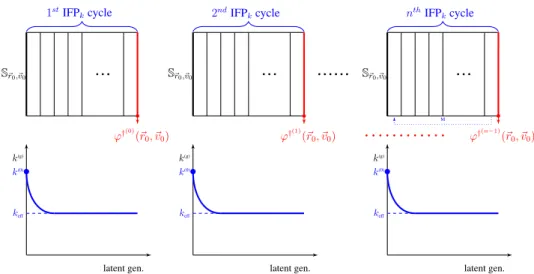
estimated by running an ensemble of B fixed-source replicas (batches) over M fission generations (see Fig. 1). For each batch, N neutrons start with coordi-natesr0,v0. The quantity M defines the IFP cycle length. If M is sufficiently

large, the neutron population (π)idescending from a common ancestor i reaches

an asymptotic distribution, and the importance Ik at generation M can be thus

95

obtained by collecting the simulation weights of all fission neutrons at genera-tion M + 1 descending from their common ancestors. To prevent the neutron population from exploding or going to extinction over the M latent generations, a rescaling factor equal to 1/k(g)_{(the multiplication factor estimated at the latent}

generation g) is applied. The quantity k(g) _{asymptotically converges to the}

fun-100

damental k-eigenvalue for a sufficiently large cycle length M, and the associated importance yields the fundamental adjoint neutron flux ϕ†

0(r0,v0) evaluated at

the phase space coordinates where the ancestor neutron has been injected (up to a normalization factor).

Actually, the algorithm implemented in Tripoli-4 R _{allows more generally} 105

computing scalar products of the kind hϕ†_{, S i, where S is an arbitrary}

user-defined source, and then decomposing the resulting scores on a spatial, energetic and angular mesh with respect to the starting coordinates of the neutrons. As a particular case, for delta-like sources at a given point in phase space we recover the adjoint flux ϕ†

0(r0,v0).

110

2.4. Determining the IFP cycle length

Selecting a proper IFP cycle length M for IFP simulations might be a difficult task (Nauchi and Kameyama, 2010; Kiedrowski et al., 2011). Longer cycles ensure a better convergence to the asymptotic behaviour, thus minimizing the approximation due to a finite number of IFP generations. On the other hand,

115

for excessively long cycles neutron histories might be killed before contributing to the final score, thus increasing the variance of the calculation. In order to

(7)

S~r0,~v0 ϕ†(0) (~r0, ~v0) S~r0,~v0 ϕ†(1) (~r0, ~v0) S~r0,~v0 ϕ†(n−1) (~r0, ~v0)

1st_IFPk_cycle ₂nd_IFPk_cycle _nth_IFPk_cycle

M keff k(0) k(g) latent gen. keff k(0) k(g) latent gen. keff k(0) k(g) latent gen.

Figure 1: The IFP method as applied to the calculation of the adjoint flux.

provide a convergence estimator for the IFP scores, we have implemented in Tripoli-4 R _{the so-called relative information entropy between two cycle lengths.}

The relative entropy, also known as the Kullback-Leibler divergence (Cover and

120

Thomas , 2006), provides a measure of the distance between two distributions. For two discrete probability distributions p and q, the relative entropy is defined as (Shannon , 1948; Cover and Thomas , 2006)

D(pkq)=X

j

p( j) log p( j)

q( j). (10) Roughly speaking, the relative entropy D(pkq) quantifies the approximation that we make by taking q(x) as a probability distribution, whereas the true distri-bution is p(x). The idea is that we can assume as a reference distridistri-bution the one which is obtained taking the longest cycle length M. This definition could be then applied to the different adjoint scores distributions πM

i and π M0

i for the

generic phase-space score bin xi, associated to two different cycle lengths M0 <

M (Truchet, 2015): p(xi)= πM i P jπMj (11) q(xi)= πM0 i P jπM 0 j . (12)

(8)

The following relative entropy for the two cycles can be estimated: D(pkq)= X i πM i P jπMj log        P jπM 0 j πM0 i πM i P jπMj        (13) = log         X j πM0 j         −log         X j πM j        + P jπM 0 j log πM j πM0 j P jπMj . (14) In the following, the simulation results for the Kullback-Leibler divergence will be normalized to the absolute entropy of the longest cycle M, defined as (Shan-non , 1948) H(p)=X x p(x) log 1 p(x) (15) = log        X i πM i        − P iπiMlog π M i P iπiM . (16) As shown in the next Sections, the D(pkq) measure has been used in the veri-fication test cases in order to determine the relative entropy for different cycle

125

lengths M and get some insight on the convergence of the IFP algorithm for different reactor configurations.

3. Verification on simple multiplying systems

In this section we will illustrate some examples of verification tests for the adjoint flux calculations that have been realized by using Tripoli-4 R_.

130

3.1. Two-group, infinite medium transport

As a first application, let us consider a homogeneous system of infinite size, with two energy groups 31 (fast) and 32 (thermal) and two delayed families a

and b. We assume, as in (Kiedrowski, 2010), that no up-scattering is possible, fissions can be induced only by neutrons colliding in the thermal group g= 2 and finally fission neutrons are emitted exclusively in g= 1. Under such conditions, the k-eigenvalue transport problem can be reduced to a system of equations for the scalar flux ϕ, namely,

Σr,1ϕk,1= 1

k(1 − βtot+ ξ1)νf,2Σf,2ϕk,2 Σr,2ϕk,2= Σs,12ϕk,1+ 1

(9)

g Σrg Σfg χa→g χb→g Σs,g→1 Σs,g→2 Σag

1 1.5 0 3/4 1/2 1/2 1/2 1

2 2 1 1/4 1/2 0 1 1.5

Table 1: The physical parameters for the two-group infinite medium system, expressed in arbi-trary units.

where ϕk,g = ϕk(3g) andΣx,g = Σx(3g). HereΣs,g j= Σs(3g → 3j) is the differential

scattering kernel, Σr,g = Σt,g − Σs,gg the removal cross-section of group g, Σf,g

the fission cross-section of group g, νf,g the number of neutrons produced by a

fission in group g, χi,g is the delayed neutron spectrum from delayed family i

to energy group g, βi the delayed neutron fraction of family i, βtot = βa + βb,

and ξg = χa,gβa+ χb,gβb. The associated adjoint equations can be obtained from

Eqs. (17) by transposition, i.e., Σr,1ϕ†_k,1 = Σs,12ϕ†_k,2 Σr,2ϕ†_k,2 = 1 k h(1 − β + ξ1)νf,2Σf,2ϕ † k,1+ ξ2νf,2Σf,2ϕ † k,2i . (18)

For this simple configuration, it is possible to derive analytical solutions for the forward flux ratio (Kiedrowski, 2010)

z= ϕ2 ϕ1 =

Σs,12

Σr,2− _k1_effξ2νf,2Σf,2

, (19)

and the adjoint flux ratio

z† = ϕ † 1 ϕ† 2 = Σ_Σs,12 r,1 , (20)

as well as the multiplication factor k= νf,2Σf,2 Σr,2

h

z†(1 − β+ ξ1)+ ξ2i . (21)

The physical parameters chosen for our simulations are reported in Tab. 1. The Tripoli-4 R _{scattering and fission kernels were modified to meet the}

specifications of the simplified model. In Fig. 2 the adjoint flux ratio ϕ† 1/ϕ

† 2 is

provided as a function of the absorption cross section of the first (fast) group.

135

(10)

For verification purposes, an IFP cycle length of M = 10 was chosen, wven if lower values were largely sufficient to achieve the convergence of the importance for this a simple configuration. The 2-group Tripoli-4 R _{results with a 2-σ error}

bar1_{have been compared to the exact solutions given in Eq. (20), showing a good}

140 agreement. 0.2 0.4 0.6 0.8 1 1.2 1.4 1.6 1.8 2 0.2 0.3 0.4 0.5 0.6 0.7 Σa,1[a.u.] Adjoin t Flux Ratio ϕ † 1 ϕ † 2 Analytical T4-2G (2σ)

Figure 2: Comparison between Tripoli-4 R _{calculations and exact solutions for the adjoint flux}

ratio as a function of the absorption cross section in the first groupΣa,1.

3.2. Mono-kinetic transport

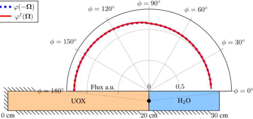
As a second application we compute the adjoint neutron flux for mono-kinetic transport. In this case, the forward and adjoint scalar fluxes are identical, while the angular fluxes are equal for opposite directions, namely,

145

ϕ(Ω) = ϕ†_(−Ω). ₍₂₃₎

This property has been conveniently used in order to verify the IFP method im-plemented in Tripoli-4 R_.

1_Tripoli-4 R _{can provide the adjoint flux for each group. The standard deviation for the ratio}

between two groups has been derived by using σ        ϕ† 1 ϕ† 2        ' v u t       1 ϕ† 2 σ(ϕ† 1)        2 +        ϕ† 1 ϕ†,2 2 σ(ϕ† 2)        2 . (22)

(11)

UOX 0cm 20cm 30cm H2O φ = 0◦ φ = 30◦ φ = 60◦ φ = 90◦ φ = 120◦ φ = 150◦ φ = 180◦ Flux a.u. 0 0.5 1 ϕ(−Ω) ϕ†_(Ω)

Figure 3: Comparison between the forward and the adjoint angular flux in opposite directions, for a mono-kinetic calculation. Results are given in arbitrary units.

The reactor configuration consists of two adjacent boxes, the former filled with fuel and the latter filled with water (see Fig. 3). Reflecting boundary con-ditions have been imposed on the faces whose normal vectors are aligned along

150

−x, ±y and ±z directions. Vacuum boundaries are imposed along the +x di-rection. The angular flux has been computed at the interface between fuel and water.

In Fig. 3 we display the comparison between the forward and the adjoint az-imuthal flux for opposite directions2_{. The simulation results show a good}

agree-155

ment between the two calculations performed by Tripoli-4 R_{, which is coherent}

with Eq. 23. A total of 105_{neutrons and 10}5_{batches have been used for both}

for-ward and adjoint simulations. For the adjoint flux, an IFP cycle length of M= 6 latent generations has been chosen. This value is to be compared with the rela-tive entropy plot presented in Fig. 4. As mentioned in the previous section, the

160

Kullback-Leibler factor D has been computed by taking as reference cycle length Mmax = 8, which was deemed to be sufficient for this simple configuration.

2_{Supposing the angular distribution described by two angles φ and θ, we show the angular}

(12)

1 2 3 4 5 6 7 8 0 0.5 1 ·10−3 IFP Cycle Rel. En trop y [%]

Figure 4: Relative entropy calculation for the mono-kinetic reactor configuration, by assuming

Mmax= 8.

4. Analysis of reactor configurations

A few realistic reactor configurations have been selected in order to probe the behaviour of the adjoint flux computed by Tripoli-4 R _{with respect to the results} 165

obtained from deterministic solvers. For each reactor test case, geometrical and material specifications are provided in order to ensure benchmark-quality results. 4.1. Simplified SFR reactor

As a first configuration, we have examined the 2D axial section of a Sodium-cooled Fast Reactor (SFR) (Truchet, 2014b). The reactor geometry is provided

170

in Fig. 5 and the compositions are given in Tab. 2. The geometry is basically made of several layers of different materials, with leakage boundary conditions on the axial direction.

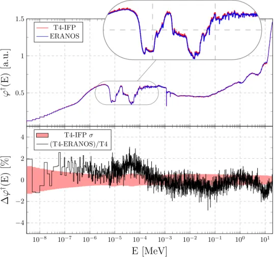
The adjoint neutron flux ϕ†_{(E) averaged on the whole geometry and}

com-puted by using Tripoli-4 R _{is illustrated in Fig. 6. The Monte Carlo} simula-175

tion results obtained with 3 × 106 _{neutrons and 5 × 10}4 _{cycles are compared}

to those of the deterministic solver ERANOS/BISTRO (Ruggieri et al., 2006) us-ing a 1968 energy group mesh with a P3 anisotropy order. The ERANOS code3

is a reactor physics calculation system including various deterministic solvers for the neutron transport equation, developed and validated for current and

ad-180

vanced fast spectrum reactor applications. In particular, the ERANOS/BISTRO

(13)

Composition 1024 cm3 Composition10 24 cm3 Top Reflector 52_Cr _1.319373E-2 56_Fe _4.875390E-2 58_Ni _4.883710E-3 60_Ni _1.895516E-3 Blanket 238_U _1.405553E-2 16_O _2.818029E-2 27_Al _4.443492E-3 52_Cr _1.127610E-3 56_Fe _4.155072E-3 58_Ni _4.161906E-4 60_Ni _1.619658E-4 Plenum 52_Cr _2.350464E-3 56_Fe _8.673668E-3 58_Ni _8.687959E-4 60_Ni _3.379375E-4 Fuel1-2-3 239_Pu _1.067352E-3 52_Cr _1.779916E-3 56_Fe _6.548571E-3 58_Ni _6.520389E-4 60_Ni _2.537198E-4 238_U _7.871417E-3 16_O _1.578161E-2 27_Al _2.488458E-3 23_Na _6.229042E-9 Bottom Reflector 52_Cr _1.127610E-3 56_Fe _4.155072E-3 58_Ni _4.161906E-4 60_Ni _1.619658E-4

(14)

Reflector 0 Blanket 50 Fuel1 79.3 Fuel2 105.4 Fuel3 131.5

Empty Sodium Plenum 157.6 Blanket 197.2 Reflector 206.9 246.9 X (cm) Axial Leakage Axial Leakage

Figure 5: 1D axial section of the Sodium-cooled Fast Reactor (SFR) configuration.

solver (Palmiotti et al. , 1990) allows finite difference Sn transport calculations with an improved convergence algorithm, which can be used in 1D and 2D ge-ometries.

The adjoint flux computed with Tripoli-4 R _{has been decomposed on an} en-185

ergy mesh exactly matching that of ERANOS/BISTRO. Spatial and angular vari-ables have been averaged out. For the Monte Carlo results, 1σ error bars are also displayed, barely visible in the top part of the figure. For the SFR configuration tested here, Tripoli-4 R _{and ERANOS provide consistent results over the whole}

energy range. This is confirmed by the reduced χ2 _{test, defined as}

190 χ2₌ 1 (G − 1) G X g=1 (ϕ† g,T4−ϕ † g,det) 2 σ2 g,T4 , (24)

where the sum is extended over the the number of energy groups G, ϕ† g,det is

(15)

0.5 1 1.5

ϕ

†

(E)

[a.u.]

T4-IFP ERANOS 10−8 ₁₀−7 ₁₀−6 ₁₀−5 ₁₀−4 ₁₀−3 ₁₀−2 ₁₀−1 ₁₀0 ₁₀1 −4 −2 0 2 4

E [MeV]

∆

ϕ

†

(E)

[%]

T4-IFP σ (T4-ERANOS)/T4

0.5

1

1.5

ϕ

†

(E)

[a.u.]

T4-IFP

ERANOS

10 −8

10 −7

10 −6

10 −5

10 −4

10 −3

10 −2

10 −1

10

0

10

1 −4

−2

0

2

4

E [MeV]

∆

ϕ

†

(E)

[%]

T4-IFP σ

(T4-ERANOS)/T4

Figure 6: Comparison between ERANOS and Tripoli-4 R _{adjoint flux calculations for an SFR-like}

simplified reactor with empty sodium plenum (top). Relative differences between Tripoli-4 R

and ERANOS are checked against the Monte Carlo 1σ-error bars (bottom).

(with associated standard deviation σg,T4). For our simulations, we have obtained

χ2 _' _{2.8 which is a satisfactory result}4_.

Note that Tripoli-4 R _{results are obtained by using continuous-energy} par-195

ticle transport, which could explain the slight differences observed. Moreover, in ERANOS the cross section self-shielding procedure used to solve the adjoint transport equation is based on the forward flux. This could be responsible of

4_{A perfect agreement is achieved when the reduced χ}2 _{test provides a result of 1. However,}

the two quantities for which the cost function χ2 _{is calculated are two adjoint fluxes obtained}

by different numerical tools. A value of 2.8 could be considered a quite satisfactory result if we consider all the approximations introduced in the deterministic solvers.

(16)

some deviations visible in the energy range corresponding to resonances. This phenomenon is expected to worsen when larger energy meshes are adopted in

200

the deterministic solvers, as shown in the following. 4.2. Sodium-cooled MOX fuel pin-cell

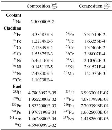
As a second configuration, we have considered a sodium-cooled MOX fuel pin-cell, whose geometry and material compositions are illustrated in Fig. 7 and Tab. 3, respectively. The adjoint neutron flux ϕ†_{(E) computed by Tripoli-4} R 205

is shown in Fig. 8: the Monte Carlo results are compared to those obtained with the deterministic code APOLLO2 using a Method of Characteristics (MOC) solver (Sanchez et al., 1988, 2010). The APOLLO2 spectral transport code al-lows cross section generation, forward and adjoint transport calculations through several deterministic solvers, i.e., collision probability method, nodal Sn and

210

short/long MOC. For both deterministic and Monte Carlo simulations, the ad-joint flux is computed on the same 281-group SHEM energy grid (Hfaiedh and Santamarina, 2005). For the Monte Carlo simulation a cycle length of M = 5 ensures convergence of the asymptotic neutron importance via IFP. For this test case 5 × 103 _{neutrons and 10}4 _{cycles were chosen for statistical accuracy. To}

215

minimize the biases between Tripoli-4 R _{and APOLLO2 due to the deterministic}

calculation options, the Monte Carlo simulation was performed in a multi-group mode. The adjoint flux ϕ†_{(E) was calculated averaging out} r and Ω5_{. A good}

agreement has been found on the whole energy range. The reduced χ2_{test yields}

χ2 _' _1.07.

220

(17)

Composition 1024 cm3 Composition 10 24 cm3 Coolant 23_Na _2.500000E-2 Cladding 54_Fe _3.38587E-3 56_Fe _5.31510E-2 57_Fe _1.22749E-3 58_Fe _1.63356E-4 50_Cr _7.12849E-4 52_Cr _1.37466E-2 53_Cr _1.55875E-3 54_Cr _3.88007E-4 58_Ni _5.46116E-3 60_Ni _2.10362E-3 61_Ni _9.14511E-5 62_Ni _2.91521E-4 64_Ni _7.42840E-5 55_Mn _1.21336E-3 59_Co _1.10738E-4 Fuel 235_U _{4.7803052E-05} 236_U _{3.9930001E-07} 238_U _{1.9522000E-02} 238_Pu _{4.0817999E-05} 239_Pu _{1.8232000E-03} 240_Pu _{7.7093998E-04} 241_Pu _{1.9767199E-04} 242_Pu _{1.6626000E-04} 241_Am _{1.4628800E-04} 237_Np _{1.4482600E-06} 16_O _{4.5940999E-02}

(18)

MOX R= 0.4098 cm 0.418cm 0.475cm

Na

(19)

0 0.5 1 1.5 2 2.5 ϕ † (E) [a.u.] T4-IFP AP2-MOC 10−9 ₁₀−8 ₁₀−7 ₁₀−6 ₁₀−5 ₁₀−4 ₁₀−3 ₁₀−2 ₁₀−1 ₁₀0 ₁₀1 ₁₀2 −30 −20 −10 0 10 20 30 E [MeV] ∆ ϕ † (E) [%] T4-IFP σ (T4-AP2)/T4

Figure 8: Comparison between Tripoli-4 R _{and APOLLO2 adjoint flux calculations for a}

sodium-cooled MOX-pin-cell (top). Relative differences between Tripoli-4 R _{and APOLLO2 are checked}

against the Monte Carlo error bars (bottom). The filled red band represents the Tripoli-4 R

(20)

4.3. UOX and MOX fuel assemblies

In order to further substantiate our analysis, we have finally considered UOX and MOX fuel assemblies representative of PWR reactors. The fuel rods are arranged in a 17 × 17 square lattice with a pitch of 1.262082 cm. Additionally, 25 water holes are located as shown in Fig. 9, while fuel rod and water channel

225

dimensions are provided in Tab. 4, where the radial mesh of the fuel pins used in the APOLLO2 calculations is also provided.

20

45

21

Figure 9: PWR 17 × 17 fuel assembly configuration. The numbering associated to the fuel pin

considered in the Tripoli-4 R_{-APOLLO2 comparisons is shown.}

MOX and UOX assemblies geometrical specifications are the same, only fuel material compositions differ. Fuel, cladding and coolant compositions for both assemblies are provided in Tab. 5.

(21)

Parameter l [cm] Parameter l [cm] Fuel Rod R1 0.26099 R2 0.34536 R3 0.36909 R4 0.39148 R5 0.40221 R6 0.41266 G 0.47436 d 1.262082 Water Channel Ri 0.56343 Re 0.6035

Table 4: Fuel rod and water holes dimensions referring to parameters given in Fig. 10. Internal radius of the spatial mesh for the fuel pin used in APOLLO2 is also given.

H2O cladding R1 R₂ R 3 R 4 R 5 R 6 G d H2O guide Ri R e

Figure 10: Fuel pin-cell and water channel guide tube dimensions. The values are provided in Tab. 4

(22)

Composition 1024 cm3 Composition10 24 cm3 Coolant at 574 K 1_H _4.771600E-2 10_B _3.972400E-6 11_B _1.589000E-5 16_O _2.385800E-2

Water Channel Guide at 574 K

54_Fe _8.626900E-6 56_Fe _1.354200E-4 57_Fe _3.127500E-6 58_Fe _4.162200E-7 50_Cr _3.279900E-6 52_Cr _6.324900E-5 53_Cr _7.172000E-6 54_Cr _1.785300E-6 16_O _3.067400E-4 90_Zr _2.171980E-2 91_Zr _4.736510E-3 92_Zr _7.239810E-3 94_Zr _7.336880E-3 96_Zr _1.181990E-3 Fuel UOX at 924 K 235_U _8.414800E-4 238_U _2.162500E-2 16_O _4.493200E-2 Fuel MOX at 924 K 234_U _3.939000E-7 235_U _4.952400E-5 238_U _2.168300E-2 238_Pu _2.224300E-5 239_Pu _7.016400E-4 240_Pu _2.713800E-4 241_Pu _1.328500E-4 242_Pu _6.698400E-5 241_Am _1.297800E-5 242m_Am _2.25690E-10 16_O _4.588200E-2 Fuel Cladding at 624 K 90_Zr _2.206000E-2 91_Zr _4.810700E-3 92_Zr _7.353200E-3 94_Zr _7.451800E-3 96_Zr _1.200500E-3

(23)

The APOLLO2-code with a P5 anisotropy and 281 groups has been used to cal-culate the deterministic adjoint flux. The Method of Characteristic made avail-able in APOLLO2 has been chosen to solve the adjoint transport equation. The Livolant-Jeanpierre technique (Sanchez et al., 2010; Jeanpierre and Livolant , 1974) has been adopted to produce shelf-shielded cross sections. The Monte

235

Carlo adjoint flux has been obtained via the IFP method in a continuous energy simulation of 5 × 104 _{neutrons using 10}5 _{batches, with an IFP cycle length of}

M = 12. The adjoint flux results averaged on the whole volume for the UOX and MOX fuels are given in Fig. 11 and 12, respectively.

0.5 1 1.5 2

ϕ

†

(E)

[a.u.]

T4-IFP AP2-MOC 10−9 ₁₀−8 ₁₀−7 ₁₀−6 ₁₀−5 ₁₀−4 ₁₀−3 ₁₀−2 ₁₀−1 ₁₀0 ₁₀1 ₁₀2 −2 0 2 4 6

E [MeV]

∆

ϕ

†

(E)

[%]

T4-IFP σ (T4-AP2)/T4 36.7 eV

0.5

1

1.5

2

ϕ

†

(E)

[a.u.]

T4-IFP

AP2-MOC

10 −9

10 −8

10 −7

10 −6

10 −5

10 −4

10 −3

10 −2

10 −1

10

0

10

1

10

2 −2

0

2

4

6

E [MeV]

∆

ϕ

†

(E)

[%]

T4-IFP σ

(T4-AP2)/T4

36.7 eV

Figure 11: Comparison between Tripoli-4 R _{and APOLLO2 adjoint flux calculations for the PWR}

assembly with UOX fuel (top). Relative differences between Tripoli-4 R _{and APOLLO2 are}

checked against the Monte Carlo error bars (bottom). The filled red band represents the

Tripoli-4 R _{1σ-statistical error.}

The χ2_{was estimated, yielding a value of χ}2 _'_{6.2 for the PWR-UOX}

assem-240

(24)

0.5 1 1.5 2

ϕ

†

(E)

[a.u.]

T4-IFP AP2-MOC 10−9 ₁₀−8 ₁₀−7 ₁₀−6 ₁₀−5 ₁₀−4 ₁₀−3 ₁₀−2 ₁₀−1 ₁₀0 ₁₀1 ₁₀2 −2 0 2 4 6

E [MeV]

∆

ϕ

†

(E)

[%]

T4-IFP σ (T4-AP2)/T4 36.7 eV

0.5

1

1.5

2

ϕ

†

(E)

[a.u.]

T4-IFP

AP2-MOC

10 −9

10 −8

10 −7

10 −6

10 −5

10 −4

10 −3

10 −2

10 −1

10

0

10

1

10

2 −2

0

2

4

6

E [MeV]

∆

ϕ

†

(E)

[%]

T4-IFP σ

(T4-AP2)/T4

36.7 eV

assembly with MOX fuel (top). Relative differences between Tripoli-4 R _{and APOLLO2 are}

checked against the Monte Carlo error bars (bottom). The filled red band represents the

Tripoli-4 R _{1σ-statistical error.}

(25)

bly and χ2 _' _{1.9 for the PWR-MOX assembly. Slight differences were detected}

between the deterministic and the Monte Carlo calculations, especially in the resonance energy region (see Figs. 11 and 12). This might probably be due to the multi-group approximation in the deterministic calculations. In particular, the same discrepancy was observed in both cases close to the 238_{U resonance}

245

at 36.7 eV, where the chosen 281-group energy mesh is actually coarser. Even if the deterministic calculation options were chosen to achieve the best perfor-mance possible, self-shielding was based on the forward flux, providing the same cross sections to both adjoint and forward transport equations.

A more significant discrepancy was observed in the fast region, i.e., E > 10

250

MeV. The fastest energy group flux shows a discrepancy between the two cal-culations, presenting a relative difference of about 5%. This discrepancy mani-fests itself also in direct criticality calculations, so that we suspect that this issue might be due to the fact that the energy grid for the deterministic solver is not fine enough in this region.

255

Another source of possible discrepancies between Tripoli-4 R _{and APOLLO2}

calculations lies in the fact that Tripoli-4 R _{uses evaluated cross section data}

at the temperatures given in Tab. 5, whereas for heavy nuclei and Zirconium APOLLO2will interpolate the data for 650 C between library tabulated values at 500and 700 C. The moderator temperature, on the contrary, coincides with a

260

tabulated value for the APOLLO2 library.

5. Local adjoint flux calculations in UOX and MOX assemblies

The previous calculations showed a satisfactory comparison between Tripoli-4 R _{and APOLLO2 for the adjoint flux averaged over the angle and the entire}

as-sembly volume. Extended simulations were performed in order to verify whether

265

local adjoint fluxes in the fuel and in the coolant do provide comparable results between the two codes, running 105 _{neutrons for 5 × 10}4 _{batches in the Monte}

Carlo simulations.

In Figs. 13, 14, 15 and 16 we illustrate the adjoint flux in the fuel pin number 20 and 456 _{for both UOX and MOX assemblies, respectively (see Fig. 9 for}

270

fuel pin numbering). The same discrepancies observed in the whole assembly calculations are now more apparent for both fuel kinds and for both pin cells, regardless of their location in the assembly lattice. The adjoint flux calculation for the pin-cell number 20 yields results similar to those obtained for pin-cell

6_{The angular adjoint flux was integrated over the solid angle and the fuel pin-cell volume}

(26)

45, although the former is closer to the water hole and the latter is located in a

275

peripheral and less moderated region. This is confirmed by the χ2 _{results given}

in Tab. 6. 0 0.5 1 1.5 2

ϕ

†

(E)

[a.u.]

T4-IFP AP2-MOC 10−9 ₁₀−8 ₁₀−7 ₁₀−6 ₁₀−5 ₁₀−4 ₁₀−3 ₁₀−2 ₁₀−1 ₁₀0 ₁₀1 ₁₀2 −5 0 5

E [MeV]

∆

ϕ

†

(E)

[%]

T4-IFP σ (T4-AP2)/T4 H2O cladding 20 UOX

0

0.5

1

1.5

2

ϕ

†

(E)

[a.u.]

T4-IFP

AP2-MOC

10 −9

10 −8

10 −7

10 −6

10 −5

10 −4

10 −3

10 −2

10 −1

10

0

10

1

10

2 −5

0

5

E [MeV]

∆

ϕ

†

(E)

[%]

T4-IFP σ

(T4-AP2)/T4

H2O cladding

20 UOX

assembly with UOX fuel, in the whole fuel pin number 20 (top). Relative differences between

Tripoli-4 R _{and APOLLO2 are checked against the Monte Carlo error bars (bottom). The filled red}

band represents the Tripoli-4 R _{1σ-statistical error. The coloured region in the fuel pin picture}

represents the volume over which the flux has been integrated.

In order to better apprehend at which spatial location within the pin-cell the discrepancy between the adjoint flux of Tripoli-4 R _{and APOLLO2 increases,}

sev-eral simulations were performed so as to estimate the adjoint flux integrated over

280

different cylindrical shells in the fuel pin of the UOX fuel assembly. In Figs. 17 and 18 the adjoint flux in the most external cylindrical shell of the fuel pin num-ber 20 is presented for both UOX and MOX assemblies, respectively (see Fig. 9 for fuel pin numbering). Although for higher energies the discrepancies

(27)

0 0.5 1 1.5 2 ϕ † (E) [a.u.] T4-IFP AP2-MOC 10−9 10−8 10−7 10−6 10−5 10−4 10−3 10−2 10−1 100 ₁₀1 ₁₀2 −10 −5 0 5 E [MeV] ∆ ϕ † (E) [%] T4-IFP σ (T4-AP2)/T4 H2O cladding 20 MOX -60%

0

0.5

1

1.5

2 ϕ

†

(E)

[a.u.]

T4-IFP

AP2-MOC

10 −9

10 −8

10 −7

10 −6

10 −5

10 −4

10 −3

10 −2

10 −1

10

0

10

1

10

2 −10

−5

0

5 E [MeV]

∆

ϕ

†

(E)

[%]

T4-IFP σ

(T4-AP2)/T4

H2O cladding

20 MOX

-60%

assembly with MOX fuel, in the whole fuel pin number 20 (top). Relative differences between

(28)

0 0.5 1 1.5 2

ϕ

†

(E)

[a.u.]

T4-IFP AP2-MOC 10−9 ₁₀−8 ₁₀−7 ₁₀−6 ₁₀−5 ₁₀−4 ₁₀−3 ₁₀−2 ₁₀−1 ₁₀0 ₁₀1 ₁₀2 −5 0 5 10

E [MeV]

∆

ϕ

†

(E)

[%]

0

0.5

1

1.5

2

ϕ

†

(E)

[a.u.]

T4-IFP

AP2-MOC

10 −9

10 −8

10 −7

10 −6

10 −5

10 −4

10 −3

10 −2

10 −1

10

0

10

1

10

2 −5

0

5

10

E [MeV]

∆

ϕ

†

(E)

[%]

T4-IFP σ

(T4-AP2)/T4

H2O cladding

45 UOX

assembly with UOX fuel, in the whole fuel pin number 45 (top). Relative differences between

(29)

0 0.5 1 1.5 2 ϕ † (E) [a.u.] T4-IFP AP2-MOC 10−9 ₁₀−8 ₁₀−7 ₁₀−6 ₁₀−5 ₁₀−4 ₁₀−3 ₁₀−2 ₁₀−1 ₁₀0 ₁₀1 ₁₀2 −10 −5 0 5 10 E [MeV] ∆ ϕ † (E) [%] T4-IFP σ (T4-AP2)/T4 H2O cladding 45 MOX -60%

0

0.5

1

1.5

2 ϕ

†

(E)

[a.u.]

T4-IFP

AP2-MOC

10 −9

10 −8

10 −7

10 −6

10 −5

10 −4

10 −3

10 −2

10 −1

10

0

10

1

10

2 −10

−5

0

5

10 E [MeV]

∆

ϕ

†

(E)

[%]

T4-IFP σ

(T4-AP2)/T4

H2O cladding

45 MOX

-60%

assembly with MOX fuel, in the whole fuel pin number 45 (top). Relative differences between

(30)

served for pin-cell calculations look the same as for the whole assembly, a clear

285

improvement in the energy region corresponding to the resonance at 36.7 eV is observed. 0 0.5 1 1.5 2

ϕ

†

(E)

[a.u.]

T4-IFP AP2-MOC 10−9 ₁₀−8 ₁₀−7 ₁₀−6 ₁₀−5 ₁₀−4 ₁₀−3 ₁₀−2 ₁₀−1 ₁₀0 ₁₀1 ₁₀2 −2 0 2 4 6

E [MeV]

∆

ϕ

†

(E)

[%]

0

0.5

1

1.5

2

ϕ

†

(E)

[a.u.]

T4-IFP

AP2-MOC

10 −9

10 −8

10 −7

10 −6

10 −5

10 −4

10 −3

10 −2

10 −1

10

0

10

1

10

2 −2

0

2

4

6

E [MeV]

∆

ϕ

†

(E)

[%]

T4-IFP σ

(T4-AP2)/T4

H2O cladding

20 UOX

assembly with UOX fuel, in the most external fuel pin cylindrical shell (top). Relative differences

between Tripoli-4 R _{and APOLLO2 are checked against the Monte Carlo error bars (bottom). The}

filled red band represents the Tripoli-4 R _{1σ-statistical error. The coloured region in the fuel pin}

picture represents the volume over which the flux has been integrated.

(31)

0 0.5 1 1.5 2 ϕ † (E) [a.u.] T4-IFP AP2-MOC 10−9 10−8 10−7 10−6 10−5 10−4 10−3 10−2 10−1 100 ₁₀1 ₁₀2 −10 −5 0 5 E [MeV] ∆ ϕ † (E) [%] T4-IFP σ (T4-AP2)/T4 H2O cladding 20 MOX -35%

0

0.5

1

1.5

2 ϕ

†

(E)

[a.u.]

T4-IFP

AP2-MOC

10 −9

10 −8

10 −7

10 −6

10 −5

10 −4

10 −3

10 −2

10 −1

10

0

10

1

10

2 −10

−5

0

5 E [MeV]

∆

ϕ

†

(E)

[%]

T4-IFP σ

(T4-AP2)/T4

H2O cladding

20 MOX

-35%

assembly with MOX fuel, in the most external fuel pin cylindrical shell (top). Relative differences

picture represents the volume over which the flux has been integrated.

(32)

Fig. 19 shows how the discrepancies between deterministic and Monte Carlo calculations increase when moving from the periphery to the center in the cylin-drical shells of the fuel pin number 20. In the central region of the fuel a

discrep-290

ancy is observed between APOLLO2 and Tripoli-4 R_{, which is also apparent in}

the χ2_{values reported in Tab. 6. This might be due to the fact that neutrons born}

in the central region of the pin-cell have a smaller probability to leave the fuel. In particular, those born with an energy close to the resonance at 36.7 eV have a significant probability to be promptly absorbed, yielding a lower value for the

295

adjoint flux. Otherwise, neutrons in the peripheral region of the pin-cell have a larger probability to scatter outside in the cladding or in the coolant, even close to 36.7 eV. The resonance region strongly affects the calculation of the adjoint flux in the central volume of the fuel pins, which justifies the noticeable discrepancies due to preparing adjoint self-shielded cross sections by using the forward flux in

300

the deterministic calculations. Actually, the self-shielding formalism of APOLLO2 is based on a forward slowing-down problem, while accounting for spatial effects using the collision probability approximation, which assumes isotropic emission sources. This might explain the discrepancies of the adjoint flux in the internal fuel regions close to the resonance energies.

305

The same analysis has been performed for the water hole number 21, whose χ2_{values are provided in Tab. 6. Simulation results are illustrated in Figs. 20 and}

21 for UOX and MOX fuels, respectively. In water, calculating the adjoint flux in the resonance energy domain does not show any significant issue: discrepancies are all included in the 2σ Monte Carlo error bars. However, a systematic albeit

310

slight difference was observed in the thermal energy domain, where the Monte Carlo adjoint flux appears to be underestimated if compared to the deterministic calculations.

(33)

0 0.5 1 1.5

ϕ

†

(E)

[a.u.]

T4-IFP AP2-MOC 0 0.5 1 1.5

ϕ

†

(E)

[a.u.]

0 0.5 1 1.5

ϕ

†

(E)

[a.u.]

0 0.5 1 1.5

ϕ

†

(E)

[a.u.]

100−6 ₁₀−5 ₁₀−4 ₁₀−3 0.5 1 1.5

E [MeV]

ϕ

†

(E)

[a.u.]

H2O cladding 20 UOX H2O cladding 20 UOX H2O cladding 20 UOX H2O cladding 20 UOX H2O cladding 20 UOX

assembly with UOX fuel, in the fuel pin number 20 and in different cylindrical shells. The coloured region in the fuel pin picture represents the volume over which the flux has been inte-grated.

(34)

0.5 1 1.5

ϕ

†

(E)

[a.u.]

T4-IFP AP2-MOC 10−9 ₁₀−8 ₁₀−7 ₁₀−6 ₁₀−5 ₁₀−4 ₁₀−3 ₁₀−2 ₁₀−1 ₁₀0 ₁₀1 ₁₀2 0 2 4 6

E [MeV]

∆

ϕ

†

(E)

[%]

T4-IFP σ (T4-AP2)/T4 H2O guide 21 H2O

0.5

1

1.5

ϕ

†

(E)

[a.u.]

T4-IFP

AP2-MOC

10 −9

10 −8

10 −7

10 −6

10 −5

10 −4

10 −3

10 −2

10 −1

10

0

10

1

10

2

0

2

4

6

E [MeV]

∆

ϕ

†

(E)

[%]

T4-IFP σ

(T4-AP2)/T4

H2O guide

21 H

₂

O

0.5

1

1.5

ϕ

†

(E)

[a.u.]

T4-IFP

AP2-MOC

10 −9

10 −8

10 −7

10 −6

10 −5

10 −4

10 −3

10 −2

10 −1

10

0

10

1

10

2

0

2

4

6

E [MeV]

∆

ϕ

†

(E)

[%]

T4-IFP σ

(T4-AP2)/T4

H2O guide

21 H

₂

O

assembly with UOX fuel, in the water hole number 21 (top). Relative differences between

(35)

0.5 1 1.5

ϕ

†

(E)

[a.u.]

T4-IFP AP2-MOC 10−9 ₁₀−8 ₁₀−7 ₁₀−6 ₁₀−5 ₁₀−4 ₁₀−3 ₁₀−2 ₁₀−1 ₁₀0 ₁₀1 ₁₀2 0 2 4 6

E [MeV]

∆

ϕ

†

(E)

[%]

T4-IFP σ (T4-AP2)/T4 H2O guide 21 H2O

0.5

1

1.5

ϕ

†

(E)

[a.u.]

T4-IFP

AP2-MOC

10 −9

10 −8

10 −7

10 −6

10 −5

10 −4

10 −3

10 −2

10 −1

10

0

10

1

10

2

0

2

4

6

E [MeV]

∆

ϕ

†

(E)

[%]

T4-IFP σ

(T4-AP2)/T4

H2O guide

21 H

₂

O

0.5

1

1.5

ϕ

†

(E)

[a.u.]

T4-IFP

AP2-MOC

10 −9

10 −8

10 −7

10 −6

10 −5

10 −4

10 −3

10 −2

10 −1

10

0

10

1

10

2

0

2

4

6

E [MeV]

∆

ϕ

†

(E)

[%]

T4-IFP σ

(T4-AP2)/T4

H2O guide

21 H

₂

O

assembly with MOX fuel, in the water hole number 21 (top). Relative differences between

(36)

χ2 _χ2

UOX fuel

Whole Assembly 6.2 Fuel pin 20 6.5

Fuel pin 45 6.2 Fuel pin 20 C1 12.0

Fuel pin 20 C2 8.6 Fuel pin 20 C3 5.7

Fuel pin 20 C4 4.4 Fuel pin 20 C5 4.3

Fuel pin 20 C6 3.9 Water hole 21 5.9

MOX fuel

Whole Assembly 1.9 Fuel pin 20 16.7

Fuel pin 45 14.2 Fuel pin 20 C6 15.7

Water hole 21 6.8

Table 6: χ2_{results for assembly adjoint flux calculations. The C}

irefers to the different cylindrical

shells of the fuel pin for APOLLO2 calculations.

Forward flux calculations were also performed in order to verify whether the observed differences between APOLLO2 and Tripoli-4 R _{for the adjoint flux} pro-315

files were comparable to those obtained in direct eigenvalue calculations. Track scores were collected by simulating 105 _{neutrons in 10}5 _{cycles with}

Tripoli-4 R _{to estimate the forward flux in the different cylindrical shells of the the fuel}

pin number 20. A comparison between the Monte Carlo and the deterministic calculations for the inner cylindrical region is shown in Fig. 22. Some

discrepan-320

cies were observed, which led a χ2 _{= 783, much higher than what we observed}

for the adjoint calculations. Large values of χ2 _{might be probably due to the}

small statistical uncertainty obtained in the Monte Carlo simulations: however, these differences clearly show that for the adjoint problem most discrepancies are induced by the neutron transport simulation. The Monte Carlo IFP algorithm

325

implemented in Tripoli-4 R _{can be then considered as reference tool for adjoint}

(37)

0 2 4 6 ·10−4

ϕ

†

(E)

[a.u.]

T4-TRACK AP2-MOC 10−11₁₀−10 ₁₀−9 ₁₀−8 ₁₀−7 ₁₀−6 ₁₀−5 ₁₀−4 ₁₀−3 ₁₀−2 ₁₀−1 ₁₀0 ₁₀1 ₁₀2 −4 −2 0 2 4

E [MeV]

∆

ϕ

†

(E)

[%]

H2O cladding 20 UOX

Figure 22: Comparison between Tripoli-4 R_{and APOLLO2 forward flux calculations for the PWR}

assembly with UOX fuel, in the inner region of the pin-cell number 20 (top). Relative differences

(38)

6. Comparing forward and adjoint flux calculations

Direct and adjoint criticality calculations correspond to intrinsically differ-ent simulation strategies, the former being based on the power iteration for the

330

eigenvalue form of the Boltzmann equation, and the latter being based on a spe-cial formulation of a fixed source transport problem. It is nonetheless interesting to compare the two approaches, which can provide complementary pieces of in-formation concerning multiplying systems. We conclude thus our analysis of the adjoint flux calculations made available in Tripoli-4 R _{by considering the} 335

performance of such algorithms. Direct and forward flux calculations based on a 281-group mesh (see Fig. 23) were run for MOX fuel pin-cell (examined in Sec. 4.2) on 10 Intel R _Xenon R _{CPUs E5-2620 at 2.0 GHz.}

10−9 ₁₀−8 ₁₀−7 ₁₀−6 ₁₀−5 ₁₀−4 ₁₀−3 ₁₀−2 ₁₀−1 ₁₀0 ₁₀1 ₁₀2 0 2 4 6 8 10 12 E [MeV] Adjoin t Flux [a.u.] T4-IFP T4-Track

ϕ(E)

ϕ

†

(E)

Figure 23: Adjoint (IFP) and forward (track estimator) flux calculations for a sodium cooled MOX-pin-cell.

Concerning the simulation options, 5 × 103 _{neutrons were simulated in 10}4

cycles in both cases. The number of latent generations for the IFP calculation

340

was set to M = 12. To compare the performances of the two calculations, the Figure of Merit (FOM) parameter

FOM= _σ1.0₂

T (25)

was estimated, where T is the computer time and σ2 _{the variance of the Monte}

(39)

flux norms, obtained by quadratic sums of the single group flux values7_{. The}

345

direct calculation shows better performances: it is slower than the adjoint cal-culation, but yields smaller statistical uncertainties. The ratio between the two FOMs turns out to be in fact

FOMϕ

FOMϕ†

!

cell

= 137, (26) which clearly shows higher efficiency performing the forward flux calculation.

The same performance indicator was used for an assembly simulation with

350

UOX fuel. The adjoint and the forward 281-group flux have been computed on the whole assembly volume, averaging out ther and Ω coordinates (see Fig. 24). 5 × 104_{neutrons were simulated for 10}5_{cycles on 100 Xeon E5-2680 V2 CPUs}

at 2.8 GHz. Although the adjoint calculation was faster than the forward one, the ratio between the two FOMs turns out to be

355 FOMϕ FOMϕ† ! assembly = 594. (27)

Not surprisingly, the IFP algorithm demands non-negligible computational efforts in terms of CPU-time when compared to direct criticality calculations. Nevertheless, adjoint criticality simulations are a powerful tool for the verifica-tion of deterministic codes and for the physical analysis of reactor configuraverifica-tions, as a complement of standard direct simulations. Moreover, it should be stressed

360

that adjoint calculations can easily estimate point-flux contributions at a given location in the phase space, a task which is prohibitively expensive for direct simulations.

7. Conclusions

In this paper we have illustrated the implementation and the verification tests

365

of the adjoint flux calculation capability in the Monte Carlo code Tripoli-4 R_,

in view of a future release. The basic IFP algorithm has been first briefly re-called, for the sake of completeness. We have then shown the adjoint flux pro-files obtained with Tripoli-4 R _{on some relevant reactor configurations,}

includ-ing a two-group infinite-medium model, mono-kinetic transport, sodium-cooled

370

7_{Both flux and standard deviation were renormalized to the same norm. The variance of the}

norm for the forward and the adjoint calculations was obtained by assuming that flux values at different energies are not correlated.

(40)

10−9 10−8 10−7 10−6 10−5 10−4 10−3 10−2 10−1 100 ₁₀1 ₁₀2 0 2 4 6 8 10 E [MeV] Adjoin t Flux [a.u.] T4-IFP T4-Track

ϕ(E)

ϕ

†

(E)

Figure 24: Adjoint (IFP) and forward (track estimator) flux calculations for a PWR assembly with UOX fuel.

fuel pin-cells and PWR assemblies in continuous-energy transport. For all tested configurations, the simulation results of Tripoli-4 R _{have been compared to exact}

solutions (where available) and to the adjoint flux profiles obtained by resorting to the deterministic solvers APOLLO2 and ERANOS. A satisfactory agreement has been found. Nonetheless, for some configurations and energy ranges, slight

dis-375

crepancies have been detected, which might come from the fact that the cross sections needed for self-shielding in the deterministic solvers have been com-puted by weighting by the direct neutron flux. Geometry and material specifica-tions have been provided, in order for the reader to possibly reproduce our results and compare them to those of other deterministic solvers or Monte Carlo codes.

380

Special emphasis has been given to the analysis of benchmark-quality UOX and MOX assemblies, where the global and local (i.e., at the scale of a single pin-cell of the lattice) adjoint flux profiles have been computed and verified against those produced by APOLLO2. Comparison with respect to direct Monte Carlo crit-icality calculations has shown that the IFP method implies higher computational

385

costs, which are balanced by the possibility of exploring a whole new domain of simulation for criticality problems (adjoint flux profiles basically inaccessible to Monte Carlo codes until the appearance of the IFP method). In this respect, a particularly attractive feature is the possibility of computing the adjoint flux in a single point of phase space.

390

(41)

α-eigenfunction adjoint calculations, along the lines of the methods proposed in (Terranova and Zoia, 2017).

Acknowledgements

TRIPOLI-4 R _{is a registered trademark of CEA. The authors wish to thank} 395

´Electricit´e de France (EDF) for partial financial support, and express their grati-tude to Dr. F. Malvagi of CEA/Saclay for fruitful discussions.

References

Bell, G. I., Glasstone, S., 1970. Nuclear reactor theory, Van Nostrand Reinhold Company.

Brun, E., et al., 2015. Ann. Nucl. Energy82, 151-160.

400

Choi, S., H., Shim, H., J., 2016. Ann. Nucl. Energy96, 287.

Cover, T., Thomas, J., 2006. Elements of information theory, Wiley-Interscience publication.

Feghhi, S. A. H., Shahriari, M., Afarideh, H., 2007. Ann. Nucl. Energy34, 514.

Feghhi, S. A. H., Shahriari, M., Afarideh, H., 2008. Ann. Nucl. Energy35, 1397.

Henry, A.F., 1975. Nuclear Reactor Analysis, The MIT Press.

405

Hfaiedh, N., Santamarina, A., 2005. In Proceedings of the MC 2015 conference, Avignon, France.

Hoogenboom, J. E., 2003. Nuc. Sci. Eng.143, 99.

Hurwitz Jr., H., 1964. In: Radkowsky, A. (Ed.), Naval Reactors Physics Handbook, vol. I. Naval Reactors, Division of Reactor Development, United States Atomic Energy Commission, pp.

410

864.

Kiedrowski, B.C., 2010. LA-UR-10-01803.

Kiedrowski, B. C., 2011. Adjoint Weighting for Continuous-Energy Monte Carlo Radiation Transport, PhD thesis, Michigan University.

Kiedrowski, B. C., Brown, F. B., Wilson, P. P. H., 2011. Nucl. Sci. Eng.68, 226.

415

Kiedrowski, B. C., Brown, F. B., 2013. Nucl. Sci. Eng.174, 227.

Lepp¨anen, J., et al., 2014. Ann. Nucl. Energy65, 272.

Jeanpierre, F., Livolant, M., 1974. CEA Report 4533.

Lux, I., Koblinger, L., 1991. Monte Carlo particle transport methods: Neutron and photon calcu-lations, CRC Press, Boca Raton.

420

Mosteller, R. D., Kiedrowski, B. C., 2011. LA-UR-11-04409, Los Alamos National Laboratory.

Nauchi, Y., Kameyama, T., 2010. J. Nucl. Sci. Technol.47, 977.

Perfetti, C. M., 2012. Advanced Monte Carlo methods for eigenvalue sensitivity coefficient

cal-culations, PhD thesis, Michigan University.

Palmiotti, G., Rieunier, J. M., Gho, C., Salvatores, M., 1990. Nucl. Sci. Eng.104, 26-33.

425

Qiu, Y., Shang, X., Tang, X., Liang, J., Wang, K., 2016. Ann. Nucl. Energy87, 228.

Ruggieri, J.-M., Tommasi, J., Lebrat, J.-F., Suteau, C., Plisson-Rieunier, D., De Saint Jean, C., Rimpault, G., Sublet, J.-C., 2006. In Proceedings of the ICAPP2006 conference, Reno, Nevada.

Sanchez, R., Mondot, J., Stankovski, Z., Cossic, A., Zmijarevic, I., 1988. Nucl. Sci. Eng.100,

430

(42)

Sanchez, R., Zmijarevic, I., Coste-Delclaux, M., Masiello, E., Santandera, S., Martinolli, E.,

Villate, L., Schwartz, N., Guler, N., 2010. Nucl. Eng. Techn.42, 474-499.

Shannon, C., 1948. The Bell System Technical Journal27, 379-423.

Shim, H. J., Kim, C. H., Kim, Y., 2011. J. Nucl. Sci. Technol.48, 1453.

435

Soodak, H., 1949. Pile kinetics. In: Goodman, G. (Ed.), The Science and Engineering of Nuclear Power, vol. II. Addison-Wesley Press, Inc., Cambridge, pp. 89102.

Terranova, N., Zoia, A., 2017. Annals of Nuclear Energy108, 57-66.

Truchet, G., et al., 2014. In Proceedings of the SNA+MC 2013 conference, Paris, France. Truchet, G., et al., 2014. In Proceedings of the Physor 2014 conference, Kyoto, Japan.

440

Truchet, G., 2015. Développements et validation de calculs á énergie continue ponderérés pqr l’importance, PhD thesis, Grenoble Alpes University.

Truchet, G., Leconte, P., Santamarina, A., Damian, F., Zoia, A., 2015. Ann. Nucl. Energy81,

17-26.

Ussachoff, L. N., 1955. In Proceedings of the 1st UN conference of the peaceful uses of atomic

445

energy, P/503, Geneva, Switzerland.

Weinberg, A.M., 1952. Am. J. Phys.20, 401-412.

Zoia A., Brun, E., 2016. Annals of Nuclear Energy90, 71-82.