Sea Ice Floe Impacts - Large Scale Basin Experiments

Publisher’s version / Version de l'éditeur:

Proceedings of the Tenth (2000) International Offshore and Polar Engineering

Conference ISOPE'00, 1, pp. 640-645, 2000

READ THESE TERMS AND CONDITIONS CAREFULLY BEFORE USING THIS WEBSITE. https://nrc-publications.canada.ca/eng/copyright

Vous avez des questions? Nous pouvons vous aider. Pour communiquer directement avec un auteur, consultez la

première page de la revue dans laquelle son article a été publié afin de trouver ses coordonnées. Si vous n’arrivez pas à les repérer, communiquez avec nous à PublicationsArchive-ArchivesPublications@nrc-cnrc.gc.ca.

Questions? Contact the NRC Publications Archive team at

PublicationsArchive-ArchivesPublications@nrc-cnrc.gc.ca. If you wish to email the authors directly, please see the first page of the publication for their contact information.

NRC Publications Archive

Archives des publications du CNRC

This publication could be one of several versions: author’s original, accepted manuscript or the publisher’s version. / La version de cette publication peut être l’une des suivantes : la version prépublication de l’auteur, la version acceptée du manuscrit ou la version de l’éditeur.

Access and use of this website and the material on it are subject to the Terms and Conditions set forth at

Sea Ice Floe Impacts - Large Scale Basin Experiments

Frederking, Robert; Timco, Garry

https://publications-cnrc.canada.ca/fra/droits

L’accès à ce site Web et l’utilisation de son contenu sont assujettis aux conditions présentées dans le site LISEZ CES CONDITIONS ATTENTIVEMENT AVANT D’UTILISER CE SITE WEB.

NRC Publications Record / Notice d'Archives des publications de CNRC:

https://nrc-publications.canada.ca/eng/view/object/?id=6250b095-9222-42b4-9b6c-c15ecc6e7581

https://publications-cnrc.canada.ca/fra/voir/objet/?id=6250b095-9222-42b4-9b6c-c15ecc6e7581

Proceedings of the Tenth (2000) International Offshore and Polar Engineering Conference ISOPE’00, Vol. 1, pp 640-645, Seattle, USA. 2000

Sea Ice Floe Impacts – Large Scale Basin Experiments

Robert Frederking and Garry Timco

Canadian Hydraulics Centre, National Research Council Ottawa, Ontario, K1A 0R6 Canada

Robert.Frederking@nrc.caGarry.Timco@nrc.ca

ABSTRACT

The impact forces produced by ice floes can be a significant factor in the design considerations for structures off the East Coast of Canada. A test program was carried out in an ice tank to investigate the force levels due to impact of isolated floes with a structure. In the tests, large floes of sea ice with a surface area of up to 60 m2 and thickness over 200 mm were grown. These floes represented actual sea ice floes, since there was no scaling of ice strength properties. These floes, with a mass up to 14 tonnes, were then accelerated to a desired speed (up 0.2 m/s) and allowed to impact against an instrumented test structure. The impact force and local pressures were measured for each impact. Impact velocity, floe mass and floe edge geometry were varied. The highest force levels measured were of the order of 50 kN at a speed of 0.2m/s. A simple analytical impact model was developed and validated with test results. It indicates that the maximum impact force was a function of the kinetic energy of the impacting floe raised to some power less than 1. The exponent and coefficient of the power relation were a function of ice floe edge geometry and the ice crushing pressure relation.

Key words: ice forces, sea ice, impact.

1. INTRODUCTION

In parts of the Grand Banks off the east coast of Canada, floating pack ice can be present for several weeks of the year (Wright, 1998). Offshore structures in these waters have to be designed to withstand the forces generated by the ice. Operational procedures of offshore production systems also have to take into account ice conditions. Ice forces on any fixed or floating offshore structure are generated by the interaction of loose ice floes colliding with the structure. For this type of interaction, little quantitative information is available to predict the ice loads.

Some work has been done to measure impact forces on bridge piers in rivers (Haynes et al. 1991; Frederking and Sayed, 1989) and jacket structures in marine environments (Wessels and Jochmann, 1990). In these studies, individual bridge piers have been instrumented to measure forces from the collision of ice floes with the piers during the spring break-up of the river ice. For jacket structures, forces on an individual pile have been measured for various ice conditions. Information is available on the ice forces, but limited information is available on the floe size and speed; hence, estimates of the kinetic

energy and impact force cannot be obtained and extrapolation of the data to other ice regimes is not possible. Controlled laboratory experiments to measure the forces of a sea ice floe colliding with a fixed structure would, however, provide needed data.

A test program was carried out at the Canadian Hydraulics Center, National Research Council of Canada in Ottawa. Large floes of saline ice grown in an ice tank were accelerated and allowed to drift freely into an instrumented plate. The full details of the experiments are described and the results are described in Frederking et al (1999). This paper provides a brief description of the tests, a summary of the results and a discussion on how to extrapolate the results to larger ice floe interactions in nature.

2. EXPERIMENTAL SETUP

The tests were carried out in the ice tank in a large environmental test chamber at the Canadian Hydraulics Centre at NRC. The tank is 21-m long by 7 -m wide by 1.2 -m deep. In this test program the objective was to study impact forces of ice floes having the same properties as sea ice in nature. Because ice growth in the tank is faster than in nature, the ice was grown from a saline solution that had a lower salinity than sea water. The resulting average salinity of the sea ice produced was about 4 o/oo and the grain structure was columnar, both of which are in good agreement with sea ice in nature (Weeks and Ackley, 1982). Ice growth started on April 3, 1998 and reached a thickness of 215 mm by April 14. From freeboard measurements it was calculated that the average bulk density of the ice was 930 kg/m2.

Conducting the test required a free floating ice sheet to impact against an instrumented structure. To obtain this condition, insulation sheets were placed on the water surface around the perimeter of the tank to prevent ice formation. The arrangement was supplemented by immersible heat tapes placed just under the insulation sheets. In this way a floating ice sheet about 12 m long and 6 m wide was grown, while keeping it free of the tank walls.

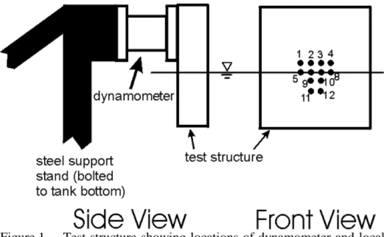
The instrumented test structure was attached to a stand that was anchored to the bottom of one end of the ice tank. The as-designed stiffness of the stand was 180 MN/m. A 45 kN capacity six-component dynamometer was placed between the test structure and the stand to measure force components in the longitudinal, transverse and vertical directions (see Figure 1). The test structure was a 12.7 mm thick framed

plate 508 mm wide by 584 mm high bolted to the front face of the dynamometer. An array of 12 local pressure sensors was placed in the front face of the test structure to provide an indication of contact area, pressure distribution and magnitude of local pressures. The sensors were spaced 50.4 mm on center and distributed on the front face of the test structure as shown in Figure 1. An accelerometer was placed on the top of the test structure to measure accelerations in the direction of ice impact. Integrating this acceleration signal twice to get displacement and comparing with the measured load, indicted a system stiffness of 18 MN/m. The combined mass of the test structure and dynamometer was about 100 kg. Using this mass, a natural frequency of 68 Hz was calculated with the measured stiffness of 18 MN/m.

Figure 1 Test structure showing locations of dynamometer and local pressure sensors

Additional instrumentation consisted of two accelerometers placed on top of the ice floe at its center, one oriented in the longitudinal direction and the other transverse. These accelerometers measured the response of the floe to impacting the test structure. A video camera was used to film a side view of each impact. The analogue signals from the dynamometer, pressure sensors and accelerometers were digitized and recorded at 1000 Hz per channel.

An overall view of the test set-up, illustrating the test structure, ice floe, accelerometer package and video camera is shown in Figure 2.

Figure 2 Overview of test set-up

3. TEST PROCEDURES AND MEASUREMENTS

Tests were run using the towing carriage in the tank to accelerate the ice sheet to a known speed, and then letting it drift under its own

momentum into the test structure. The test variables included impact speed, shape of the ice edge contacting the test structure and mass of the ice sheet. Five different ice edge geometries were prepared by making vertical saw cuts, straight, curved, 90o wedge and truncated 90o wedge (narrow tip). The geometries of the ice edges are illustrated in Figure 3. A total of 52 impact tests were conducted over a 3 day period. The size of the floe was halved twice, so that floes of three lengths, 11.9 m, 6.5m and 3.5 m, were used. For a floe width of 5.75 m and thickness of 225 mm, nominal masses of 14.3, 7.8 and 4.1 tonnes were calculated.

r =1.5 m r =3.0 m 90° wedge Straight Edge 40 mm 90° 90°

Figure 3 Geometries of ice edges

4. RESULTS

The analysis results of impact velocity and duration, floe mass, and maximum values of force and acceleration are presented in Table 1. In the cases of Tests 7, 8, 9 and 10 the dynomometer was overloaded. The overloading occurred because of large moments imposed on the dynamometer due to the need to keep it above the water surface. In these tests the maximum force was inferred from the maximum acceleration and the floe mass. The rationale for doing this will be discussed in the next section. Measured impact velocity was determined from analysis of the video records. Detailed plots of time series of resultant force on the test structure measured by the dynamometer, deceleration of the floe in the x-direction as measured with the accelerometer, and pressures measured by the pressure sensors can be found in Frederking et al (1999).

4.1 Representative Test

To illustrate the test results those of Test 20 will be presented in detail. This test involved the impact of a 14 tonne floe with a 90o wedge edge at a velocity of 114 mm/s. The force-time record measured with the dynamometer is presented in Figure 4. The force in the x-direction is the predominant force, as expected, with very little force in the y-direction. This was typical of all tests. Note that the increase of force was not smooth, that is, there were local failures of the ice that resulted in a saw-tooth characteristic in the force-time record. This force time behaviour is characteristic of the higher speed impacts with the 90o wedge-shaped edge. Viewing the video record showed visible crushing failure of the leading edge of the ice. Lower velocity impacts with the wedged-shaped edge and all impacts with the circular edge had a force-time record with a smoother sinusoidal shape.

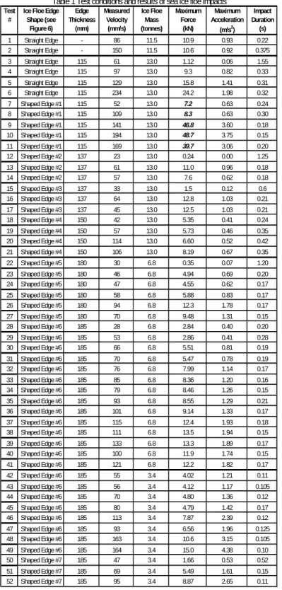
Test #

Ice Floe Edge Shape (see Figure 6) Edge Thickness (mm) Measured Velocity (mm/s) Ice Floe Mass (tonnes) Maximum Force (kN) Maximum Acceleration (m/s2₎ Impact Duration (s) 1 Straight Edge - 86 11.5 10.9 0.93 0.22 2 Straight Edge - 150 11.5 10.6 0.92 0.375 3 Straight Edge 115 61 13.0 1.12 0.06 1.55 4 Straight Edge 115 97 13.0 9.3 0.82 0.33 5 Straight Edge 115 129 13.0 15.8 1.41 0.31 6 Straight Edge 115 234 13.0 24.2 1.98 0.32 7 Shaped Edge #1 115 52 13.0 7.2 0.63 0.24 8 Shaped Edge #1 115 109 13.0 8.3 0.63 0.30 9 Shaped Edge #1 115 141 13.0 46.8 3.60 0.18 10 Shaped Edge #1 115 194 13.0 48.7 3.75 0.15 11 Shaped Edge #1 115 169 13.0 39.7 3.06 0.20 12 Shaped Edge #2 137 23 13.0 0.24 0.00 1.25 13 Shaped Edge #2 137 61 13.0 11.0 0.96 0.18 14 Shaped Edge #2 137 57 13.0 7.6 0.62 0.18 15 Shaped Edge #3 137 33 13.0 1.5 0.12 0.6 16 Shaped Edge #3 137 64 13.0 12.8 1.03 0.21 17 Shaped Edge #3 137 45 13.0 12.5 1.03 0.21 18 Shaped Edge #4 150 42 13.0 5.35 0.41 0.24 19 Shaped Edge #4 150 57 13.0 5.73 0.46 0.35 20 Shaped Edge #4 150 114 13.0 6.60 0.52 0.42 21 Shaped Edge #4 150 106 13.0 8.19 0.67 0.35 22 Shaped Edge #5 180 30 6.8 0.35 0.07 1.20 23 Shaped Edge #5 180 46 6.8 4.94 0.69 0.20 24 Shaped Edge #5 180 47 6.8 4.55 0.62 0.17 25 Shaped Edge #5 180 58 6.8 5.88 0.83 0.17 26 Shaped Edge #5 180 94 6.8 12.3 1.78 0.17 27 Shaped Edge #5 180 70 6.8 9.48 1.31 0.15 28 Shaped Edge #6 185 28 6.8 2.84 0.40 0.20 29 Shaped Edge #6 185 53 6.8 2.86 0.41 0.28 30 Shaped Edge #6 185 66 6.8 5.51 0.81 0.19 31 Shaped Edge #6 185 70 6.8 5.47 0.78 0.19 32 Shaped Edge #6 185 76 6.8 7.99 1.14 0.17 33 Shaped Edge #6 185 85 6.8 8.36 1.20 0.16 34 Shaped Edge #6 185 79 6.8 8.46 1.26 0.15 35 Shaped Edge #6 185 93 6.8 8.55 1.29 0.21 36 Shaped Edge #6 185 101 6.8 9.14 1.33 0.17 37 Shaped Edge #6 185 115 6.8 12.4 1.93 0.18 38 Shaped Edge #6 185 111 6.8 13.5 1.94 0.15 39 Shaped Edge #6 185 133 6.8 13.3 1.89 0.17 40 Shaped Edge #6 185 100 6.8 11.9 1.74 0.15 41 Shaped Edge #6 185 121 6.8 12.2 1.82 0.17 42 Shaped Edge #6 185 55 3.4 4.02 1.21 0.11 43 Shaped Edge #6 185 56 3.4 4.12 1.17 0.105 44 Shaped Edge #6 185 70 3.4 4.80 1.36 0.12 45 Shaped Edge #6 185 80 3.4 4.79 1.42 0.17 46 Shaped Edge #6 185 113 3.4 7.87 2.39 0.12 47 Shaped Edge #6 185 93 3.4 6.56 1.96 0.125 48 Shaped Edge #6 185 163 3.4 10.6 3.15 0.105 49 Shaped Edge #6 185 164 3.4 15.0 4.38 0.10 50 Shaped Edge #7 185 47 3.4 1.66 0.53 0.52 51 Shaped Edge #7 185 69 3.4 5.49 1.61 0.15 52 Shaped Edge #7 185 95 3.4 8.87 2.65 0.11

Table 1 Test conditions and results of sea ice floe impacts

The other fundamental parameter that was measured was the acceleration of the floe. Figure 5 is a plot of acceleration in the direction of floe motion versus time. In this instance the acceleration has a large high frequency component at a frequency of about 100 Hz. The accelerometer was located at the centre of the 12-m long floe. Taking a time of 0.01 s for a compression wave to travel from the centre of the floe to one end and back again (12 m), this would correspond to an acoustic velocity of about 1200 m/s. An elastic modulus of about 1 to 1.5 GPa, a reasonable value for warm sea ice, would give this value

of acoustic velocity. Because of the high frequency component in the acceleration, a moving average technique was applied to obtain a “smoothed” acceleration. This smoothed acceleration reflects the measured force of Figure 4 on a 1:1 basis throughout the test. This 1:1 correspondence was seen in all tests except Tests 7 through 10. When the measured force was divided by the floe acceleration, an “effective” floe mass was obtained. This effective mass includes the added mass of the water moving with the floe. However the velocities of the test were relatively low, so added mass is not considered to be significant in these tests. 0 1 2 3 4 5 6 7 0 0.1 0.2 0.3 0.4 0.5 time (s) forc e (k N) Fx Fy

Figure 4 Ice impact forces measured in x- and y-directions with dynomometer, Test 20 -0.6 -0.5 -0.4 -0.3 -0.2 -0.1 0 0.1 0.2 0 0.1 0.2 0.3 0.4 0.5 time (s) acceler at ion ( m/s² ) and velocit y ( m/s) velocity (m/s) "smoothed" acceleration (m/s²)

Figure 5 Acceleration (m/s2) and velocity (m/s) as a function of time in Test 20

Also shown on Figure 5 is a velocity calculated from the acceleration, starting with an initial impact velocity of 0.114 m/s. The time to zero velocity is a bit shorter than the time to zero acceleration, implying that the calculated initial impact velocity was a bit too small. Integrating the velocity gave a penetration of about 25 mm, a value that corresponds to that observed in the video.

Local pressures were also measured with pressure sensors installed in the test structure. From Figure 1 it can be seen that 12 sensors were installed in the face but, because of the water level, only 8 had the possibility of responding to ice impacts. For Test 20, only one local ice pressure was sensed, with sensor PC6. The output of sensor PC6,

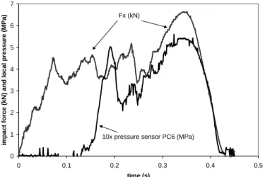
together with Fx, is plotted in Figure 6. The maximum average pressure on the 12.5-mm diameter active face of the local pressure sensor was about 0.5 MPa, and the maximum force was 6.6 kN. It can be seen that in the initial part of the impact, ice did not contact the sensor but, as the impact proceeded beyond time 0.15 s, sensor PC6 began to respond to local ice pressures, and follows the trend of the force, Fx.

0 1 2 3 4 5 6 7 0 0.1 0.2 0.3 0.4 0.5 time (s) impact f o rce ( k N ) and local pr essur e ( M P a )

10x pressure sensor PC6 (MPa) Fx (kN)

Figure 6 Comparison of impact force and local pressure on sensor PC6 for Test 20

Given the geometry of the ice edge (90o wedge) and knowing the penetration of the test structure into the ice edge (integrating the velocity of Figure 5) and the ice edge thickness, in this case 150 mm, the nominal contact area between the ice and the structure can be determined. With this area and the measured force, Fx, average pressure over the contact face can be calculated and a pressure-area curve calculated, see Figure 7. The figure shows the descending “process” pressure-area characteristic of many impact scenarios (Frederking, 1998). The average pressure during the latter part of the impact is similar to that measured by the local pressure sensor, about 0.5 MPa (see Figure 6).

0 0.5 1 1.5 2 2.5 3 0 0.002 0.004 0.006 0.008 0.01 area (m²) aver age pr essur e ( M P a ) Time

Figure 7 Pressure-area variation for Test 20 4.2 Trends of Test Results

Plotting the data of maximum force versus maximum acceleration of the three sizes of floes, mass of each size of floe could be inferred from the slope of the best fit lines. The floes masses inferred from the slopes are 13, 6.8 and 3.4 tonnes, as compared to 14.3, 7.8 and 4.1 tonnes

calculated from the dimensions of the floes. It was this mass of 13 tonnes, and the maximum accelerations that were used to determine the maximum impact forces for Tests 7 through 10. The actual masses were smaller than the masses calculated from the dimensions of the ice floe because it was assumed the thickness measured at the floe center was uniform over the entire floe. However, the thickness of the ice was less around the edges and the floes were not perfectly rectangular. Once the actual floe masses were known, the kinetic energy, KE, for each test was calculated using:

KE = ½ mV2 ₍₁₎

where m is ice floe mass and V is ice floe impact velocity. The maximum force is plotted in Figure 8 as a function of kinetic energy for the 13 tonne floe, with separate symbols being used for each edge geometry. A general trend of increasing impact force with increasing kinetic energy is observed. Best fit lines from the origin have been fit through the results for each edge geometry. With the exception of the straight edge case, the 90o wedge results in lower maximum impact forces than for the curved edges for the 13 tonne floe as well as the other two smaller floes. The geometry of the wedge with its sharp tip is most likely responsible for the lower impact forces.

Fx = 0.10 KE 90° wedge Fx = 0.22 KE 1.5-m radius Fx = 0.56 KE 3-m radius Fx = 0.079 KE straight edge 0 10 20 30 40 50 0 50 100 150 200 250 300 350 400 Kinetic Energy (J) Maximum f o rce ( k N ) straight edge 1.5-m radius 3-m radius 90° wedge

Figure 8 Maximum impact force as a function of kinetic energy for impacts of 13-t floe with various edge geometries.

0 0.2 0.4 0.6 0.8 1 1.2 1.4 1.6 0 10 20 30 40 50

Maximum Impact Force (kN)

Im pact D u rati on (s) straight R = 1.5 R = 3 90°

Figure 9 Relation between impact duration and maximum impact

Another trend that was examined was that between the maximum impact force and the impact duration. Figure 9 plots these data with different symbols for each edge geometry tested. Note that only data for the two larger floe sizes are included since only a single edge geometry was tested for the 3.4 tonne floe (90o wedge). For each edge geometry lower impact forces corresponded to longer impact durations.

5. IMPACT ANALYSIS

It is possible to make some predictions about maximum impact force as a function of kinetic energy. To do this, some assumption has to be made concerning the “crushing pressure”, p, of the ice. One possibility is to assume a constant crushing pressure, p = po, for the ice and convert all the kinetic energy to crushing of the ice. Another possibility is to assume that p, is a function of contact area, A, and is described by the following relation

p = po (A/Ao)α (2)

where α is a constant, usually experimentally determined to be 0.4 or 0.5 (Riska, 1987). For the purpose of conducting some calculations, two edge geometries will be considered, a 90o wedge and a circular edge of a constant radius. It is assumed that as the ice crushes it “disappears”, and consequently the contact area is defined by a geometric relation for the ice edge projected area on the structure (vertical plane). The approach here is similar to that of Brown and Daley (1999). For the case of the 90o wedge the contact area A, is described by

A = 2 h x (3)

where h is ice edge thickness and x in the amount of advance or penetration of the tip of the wedge into the structure. For the case of a circular edge of radius R, the contact area A is described by

A = 2 h (R2 – (R – x)2)1/2

≅ 2 h (2 R x)1/2 ₍₄₎

where, h is ice edge thickness and x in the amount of penetration of the ice edge, in this case circular in form, into the structure.

The crushing force F, for any edge geometry is given by

F = p A (5)

The energy of ice crushing CE, is given by ∫

= Fdx

CE (6)

Equating crushing energy, CE, from Equation (6) to kinetic energy, KE from Equation (1) the maximum depth of penetration, x, can be determined as a function of the ice crushing pressure relation (Equation (2)) and the ice edge geometry. Substituting the maximum penetration, x, into Equations (3) or (4) and then using Equation (5) the maximum force can be determined. For the case of a constant crushing pressure, α = 0, this system of equations can be solved in close form. For non-integer values of α, numerical integration can be used to solve for the relation between Kinetic Energy and maximum impact force.

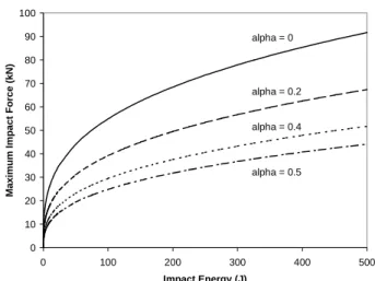
In the above analysis there are two factors that can affect the impact forces, (i) geometry of the ice edge and (ii) the crushing pressure of the ice ( α and po). To develop an appreciation for the affect of these factors a small parameter study was conducted. Figure 10 shows the affect of geometry on the maximum impact force for the cases of constant ice

crushing pressure. It can be seen that the smaller the radius of curvature or pointedness of the contact edge geometry, the lower the maximum impact force. A similar trend was obtained when a pressure-area relation with α = 0.4 or 0.5 was used. The geometry effect extends the impact duration and thus reduces the maximum force. In Figure 11 the affect of varying the exponent α in the pressure-area relation was presented. Increasing the value of α is seen to decrease the impact force. Increasing α “softens” the ice, increasing the impact duration and thus reduces the impact force. A similar effect was seen with the crushing pressure po; i.e. decreasing po softens the ice, increasing the impact duration and reducing the maximum impact force. In all cases examined, the rate of increase of the maximum impact force decreased with increasing impact energy. In fact, a simple power law relation with an exponent less that 1 described the relation. For constant ice crushing pressure, p = po (α= 0), the exponent for a circular edge was 0.33 and for the 90o wedge, 0.5. When ice crushing pressure is not constant, say α = 0.5, the exponents become 0.4 for a circular edge and 0.67 for a 90o wedge.

constant crushing pressure; po = 2000 kPa

0 10 20 30 40 50 60 70 80 90 100 0 100 200 300 400 500 Impact Energy (J) Maximum Impact For ce ( k N ) R = 1.5 R = 0.15 Wedge

Figure 10 Effect of edge geometry on the analytical relation between maximum impact force and impact energy.

0 10 20 30 40 50 60 70 80 90 100 0 100 200 300 400 500 Impact Energy (J) Maximum Impact For ce ( k N ) alpha = 0 alpha = 0.2 alpha = 0.4 alpha = 0.5

Figure 11 Effect of exponent α in the pressure area relation on the analytical relation between maximum impact force and impact energy.

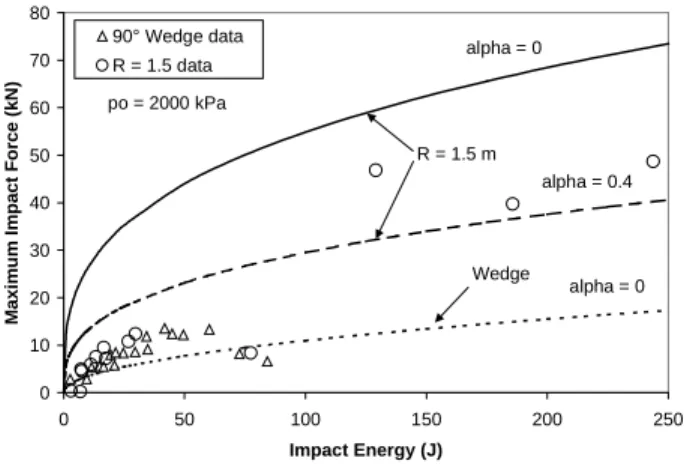
Trends in the effect of edge geometry and crushing pressure have been explored, but now they will be compared to the data measured in the tests. Figure 12 plots the measured data for all the floe impacts with the 90o wedge and circular edge of radius r = 1.5 m. For comparison the

maximum impact force predictions using the method described here are also plotted on the figure. In this case po = 2000 kPa and an edge thickness of 150 mm were used in the calculations. For the 90o wedge geometry, the predicted curve generally describes the test data. For the circular edge, the case of α = 0 and po = 2000 kPa over-predicts the data while α = 0.4 came closer to the test data. The values of po and α were selected on the basis of experience and not to provide a good fit to the experimental data. However it can be seen that there is a broad correspondence between the test results and the predictions. Perhaps most encouraging is the trend of decreasing rate of increase of the maximum impact force with increasing impact energy.

po = 2000 kPa 0 10 20 30 40 50 60 70 80 0 50 100 150 200 250 Impact Energy (J) Maximum Impact For ce ( k N ) 90° Wedge data R = 1.5 data R = 1.5 m Wedge alpha = 0 alpha = 0.4 alpha = 0

Figure 12 Comparison of measured and predicted maximum impact energy as a function of impact energy.

6. SUMMARY AND CONCLUSIONS

The results of 52 impact tests with ice floes of varying shapes and sizes have produced a substantial body of data on impact forces, floe accelerations and local pressures. The combination of floe acceleration and independent impact force measurement is a unique data set, which also provided a means of determining the actual floe mass.

Three floe sizes were tested, 13 t, 6.8 t and 3.4 t, and impact velocities ranged from 23 mm/s to 234 mm/s. Three basic edge geometries were used, a 90o wedge, 3- and 1.5-m radius and a straight edge. The maximum impact force measured was 50 kN for a kinetic energy of about 200 J. The experiments demonstrate that ice impact tests with floes of significant mass can be conducted in a relatively small facility. A simple analytical model for ice floe impact with a structure was developed. The effect of floe edge geometry and the ice crushing pressure relation was taken into account and found to be significant. The maximum impact force as a function of the kinetic energy of impact was found to a power function with exponent less than 1. The exponent and coefficient of the power relation were a function of ice floe edge geometry and the ice crushing pressure relation. The experimental data supported the trends of the analytical model.

7. ACKNOWLEDGEMENTS

The assistance of Stephen Reid, Work Term Student from Memorial University of Newfoundland in designing the tests equipment, conducting the tests and processing the test data is gratefully acknowledged. Funding support from the Program of Energy Research and Development of the Government of Canada is acknowledged.

8. REFERENCES

Brown, R. and Daley, C. 1999. Computer simulation of Transverse Ship-Ice Collisions. Report of Faculty of Engineering and Applied Science, Memorial University of Newfoundland to National Research Council for Program of Energy Research and Development, PERD/CHC Report 9-79, March 1999.

Frederking and Sayed, 1989. Measurement of Ice Impact Forces on a Vertically Faced Bridge Pier. Proceeding 8th International Offshore Mechanics and Arctic Engineering conference, The Hague, Netherlands, March 19-23, 1989, Vol. 4, pp. 319-322.

Frederking, R. 1998. The Pressure Area Relation in the Definition of Ice Forces. 8th International Offshore and Polar Engineering Conference, May 24-29, 1998, Montreal, Vol. II, pp. 431-437.

Frederking, R., Timco, G.W. and Reid, S. 1999. Sea Ice Floe Impact Experiments. National Research Council, Canadian Hydraulics Centre, Technical Report HYD-TR-038, March 1999, Ottawa, ON, Canada. Haynes, F.D., Sodhi, D.S., Zabilanski, L.J. and Clark, C.H., 1991. Ice Force Measurements on a Bridge Pier in the St. Regis River, New York. CRREL Special Report No. SR91-14, 6 pp, Hanover, HN, USA. Riska, K., 1987. On the Mechanics of the Ramming Interaction Between a Ship and a Massive Ice Floe. Thesis for degree of Doctor of Technology, Technical Research Centre of Finland, Publication 43, Espoo, Finland.

Wessels, E. and Jochmann, P., 1990. Determination of Ice Forces on Jacket JZ-20-2-1 by Model and Full Scale Tests. Hansa – Schiffahrt-Schiffbau_Hafen, 127 Jahrgang, Nr. 22, pp 1567-1570.

Weeks, W.F. and Ackley, S.F., 1982. The Growth, Structure and Properties of Sea Ice. USA CRREL Monograph 82-1, Hanover, NH, USA.

Wright, B.D., 1998. Moored Vessel Stationkeeping in Grand Banks Pack Ice Conditions. Report by B. Wright & Associates Ltd., Canatec Consultants Ltd. and AKAC Inc. to the National Research Council for the Program of Energy Research and Development, Report No. PERD/CHC 26-189, March 1998.