Buoyancy-driven circulation in the Red Sea

Buoyancy-Driven Circulation in the Red Sea

By

Ping Zhai

Submitted in partial fulfillment of the requirements for the degree of

Doctor of Philosophy in Physical Oceanography

at the

MASSACHUSETTS INSTITUTE OF TECHNOLOGY

and the

WOODS HOLE OCEANOGRAPHIC INSTITUTION

September 2014

© Ping Zhai 2014. All rights reserved.

The author hereby grants to MIT and WHOI permission to reproduce and

to distribute publicly paper and electronic copies of this thesis document

in whole or in part in any medium now known or hereafter created.

Signature of Author

. . . . . .

Joint Program in Oceanography – Massachusetts Institute of Technology /

Woods Hole Oceanographic Institution

June 16, 2014

Certified by

. . . . . .

Amy S. Bower

Senior Scientist, Woods Hole Oceanographic Institution

Thesis Supervisor

Certified by

. . .

Lawrence J. Pratt

Senior Scientist, Woods Hole Oceanographic Institution

Thesis Supervisor

Accepted by

. . .

Buoyancy-Driven Circulation in the Red Sea

by

Ping Zhai

Abstract

This thesis explores the buoyancy-driven circulation in the Red Sea, using a combination of observations, as well as numerical modeling and analytical method.

The first part of the thesis investigates the formation mechanism and spreading of Red Sea Overflow Water (RSOW) in the Red Sea. The preconditions required for open-ocean convection, which is suggested to be the formation mechanism of RSOW, are examined. The RSOW is identified and tracked as a layer with minimum potential vorticity and maximum chlorofluorocarbon-12. The pathway of the RSOW is also explored using numerical simulation. If diffusivity is not considered, the production rate of the RSOW is estimated to be 0.63 Sv using Walin’s method. By comparing this 0.63 Sv to the actual RSOW transport at the Strait of Bab el Mandeb, it is implied that the vertical diffusivity is about _3.4105_m2_s1_.

The second part of the thesis studies buoyancy-forced circulation in an idealized Red Sea. Buoyancy-loss driven circulation in marginal seas is usually dominated by cyclonic boundary currents on f-plane, as suggested by previous observations and numerical modeling. This thesis suggests that by including β-effect and buoyancy loss that increases linearly with latitude, the resultant mean Red Sea circulation consists of an anticyclonic gyre in the south and a cyclonic gyre in the north. In mid-basin, the northward surface flow crosses from the western boundary to the eastern boundary. The observational support is also reviewed. The mechanism that controls the crossover of boundary currents is further explored using an ad hoc analytical model based on PV dynamics. This ad hoc analytical model successfully predicts the crossover latitude of boundary currents. It suggests that the competition between advection of planetary vorticity and buoyancy-loss related term determines the crossover latitude.

The third part of the thesis investigates three mechanisms that might account for eddy generation in the Red Sea, by conducting a series of numerical experiments. The three mechanisms are: i) baroclinic instability; ii) meridional structure of surface buoyancy losses; iii) cross-basin wind fields.

Thesis Supervisor: Amy S. Bower

Title: Senior Scientist, Woods Hole Oceanographic Institution Thesis Supervisor: Lawrence J. Pratt

Acknowledgement

I am deeply grateful to my advisors, Amy Bower and Larry Pratt, for supporting me during my PhD studies. They always patiently supervised me and guided me in the right direction. They not only gave me helpful suggestions when I had problems about the science, but also gave me moral support to help me get through some hard times. Their creativity, broadness, and enthusiasm to science will always be an inspiration for me.

I thank my thesis committee: Paola Rizzoli, Jiayan Yang, and Tom Farrar, for their valuable guidance, brilliant comments, and consistent encouragement I received throughout the research work. I also would like to thank my thesis defense chair Claudia Cenedese. Claudia provided many useful feedbacks.

I would also like to express my sincere gratitude to Ruixin Huang and his wife Luping Zou. Xin gave me many advices on how to be a independent researcher. Luping, a good friend, taught me wisdom of life. I would also like to thank Dexing Wu and Xiaopei Lin in Ocean University of China for their guidance and help during my study in Ocean University of China.

I have had many wonderful friends and classmates in the Joint Program. I would like to thank all of you.

Finally, special thanks to my parents and my brother for supporting me through all these tough years. I would not be able to finish the PhD study without their encouragement.

This work is supported by Award Nos. USA 00002, KSA 00011 and KSA 00011/02 made by King Abdullah University of Science and Technology (KAUST) , National Science Foundation OCE0927017, and WHOI Academic Program Office.

Contents

Chapter 1 Introduction and Background ... 11 

1.1 Water masses in the Red Sea ... 13

1.1.1 RSSW ... 14

1.1.2 RSOW ... 17

1.1.3 GAIW ... 18

1.1.4 RSDW ... 21

1.2 Overturning circulations in the Red Sea ... 23

1.3 Thesis Outline ... 26

Chapter 2 Red Sea Overflow Water Formation and its Spreading Pathways ... 29 

2.2 Data ... 32

2.2.1 Hydrographic and CFC-12 data ... 32

2.2.2 Sea Surface Temperature ... 37

2.2.3 Sea Surface Heat Flux ... 38

2.2.4 QuikSCAT and ASCAT Winds ... 38

2.3 Preconditioning of Open- Ocean Convection in the Northern Red Sea ... 39

2.4 Observations of the RSOW in the Red Sea ... 49

2.5 Production Rate of RSOW ... 60

2.6 The Spreading of the RSOW in Numerical Simulations ... 69

2.7 Summary and Discussion ... 79

Chapter 3 On the Crossover of Boundary Currents in an Idealized Model of the Red Sea 85  3.1 Introduction ... 85

3.2 Numerical Model Simulation of the Buoyancy-Driven Circulation in an Idealized Red Sea ... 92

3.2.1 Model Description ... 92

3.2.2 Numerical Model Results ... 97

3.3.2 An ad hoc analytical model of Crossover Latitude ... 107

3.4 Summary and Conclusions ... 123

Chapter 4

4.1 Introduction ... 131

4.2 Eddies Generated by Baroclinic Instability ... 134

4.3 Quasi-stationary Eddies Generated by Meridional Structure of Surface Buoyancy Forcing ... 147

4.4 Eddies Generated by Cross-Basin Wind Jets ... 156

4.5 Conclusion ... 160

Chapter 5 Summary and Discussion ... 165 

5.1 Summary of Major Findings ... 165

5.2 Limitations and Future Directions ... 169

Appendix A Relation between Boundary Current and Interior Densities ... 171   

Chapter 1

Introduction and Background

The Red Sea is a semi-enclosed marginal sea, connected to the Indian Ocean via the narrow, shallow Strait of Bab el Mandeb. It presents many of the same features as other marginal seas, such as the Mediterranean Sea and the Labrador Sea. There is often net buoyancy loss to the atmosphere in marginal seas, due to heat flux, fresh water flux or both. Buoyancy loss over marginal seas can produce dense intermediate and deep water masses, which feed the deep branch of the global thermohaline circulation. These water masses usually hold distinct water properties. The Red Sea Overflow Water (RSOW), which is formed in the northern Red Sea due to surface buoyancy loss, can be tracked in the Indian Ocean as a salinity maximum. On the other hand, the Red Sea has its own unique characteristics compared to other marginal seas. The large meridional extent of the Red Sea suggests that β-effect could be more important than in other marginal seas. As a result, the Red Sea circulation could be very different from other marginal seas. Although RSOW is one of the most saline water masses in the world ocean, it cannot sink to the bottom of the Indian Ocean because it entrains very light ambient water (Price and Baringer, 1994; Bower et al., 2000). The Red Sea is a major route for commercial ships between Europe and East Asia. The Red Sea also has one of the most diverse coral reefs in the world. In addition, the Red Sea is a geologically young widening basin and it might become an ocean in the future. These unique features make the Red Sea a very interesting basin to study. However, the Red Sea circulation remains largely unexplored. In this chapter, I will review previous studies on Red Sea water masses and circulation.

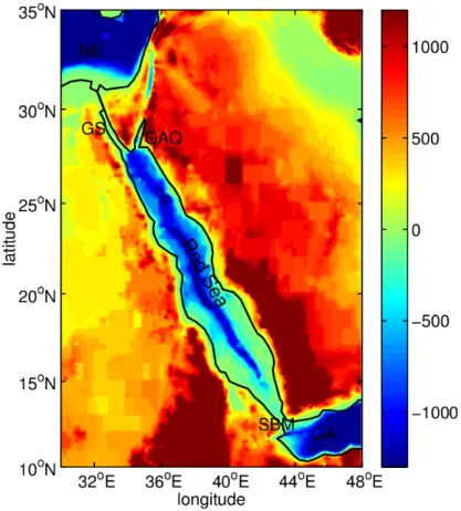
The Red Sea is a long and narrow basin that is located between Africa and Asia (Figure 1.1). It extends from 12.5°N to 30°N, a distance of about 2250 km, and has an average width of about 280km. The average depth is about 490 m, but the maximum depth along the middle axis can exceed 2000 m. The Red Sea is connected to the Indian Ocean through the Strait of Bab el Mandeb, and to the Mediterranean Sea through the Suez Canal. At about 28°N, the Red Sea splits into the Gulf of Suez and Gulf of Aqaba. At the southern end (about 12°N), the Red Sea has a minimum width of about 18 km (Murray and Johns, 1997) at the Perim Narrows in the Strait of Bab el Mandeb. The Hanish Sill, a shallow sill with a maximum depth of 137 m (Werner and Lange, 1975), is present at 13.7°N, slightly north of the Strait of Bab el Mandeb.

Both wind and buoyancy forcing have been suggested as important drivers of Red Sea circulation. The surface winds over the Red Sea blow mainly along the axis of the basin due to the high mountains on both sides. North of 18-19°N, winds blow southeastward throughout the year. In contrast, winds in the southern Red Sea are strongly influenced by the Indian monsoon system. South of 18-19°N, the wind direction changes seasonally from southeasterly during the winter monsoon season to northwesterly during the summer monsoon season (Pedgley, 1972).

Due to high evaporation, negligible precipitation, and no river runoff, the Red Sea is one of the most saline basins in the world. Heat and freshwater fluxes over the Red Sea must be balanced by heat and freshwater transports through the Strait of Bab el Mandeb. Using this constraint, combined with current and water property data measured at the Strait of Bab el Mandeb, Sofianos et al. (2002) estimate that the annual mean heat and freshwater losses to the atmosphere are

2

m W 5

11  and _{2.060.22myr}1_{, respectively. Based on results from numerical experiments}

Red Sea is primarily driven by surface buoyancy losses due to surface heat loss and evaporation. This thesis will focus on buoyancy-driven circulation.

Figure 1.1: Topographic map of the Red Sea. The colors represent elevation and bathymetric values (m). The locations of Gulf of Aqaba (GAQ), Gulf of Suez (GS), Gulf of Aden (GA), Mediterranean Sea (ME), and Strait of Bab el Mandeb (SBM) are shown.

1.1 Water masses in the Red Sea

The main water masses in the Red Sea are Red Sea Surface Water (RSSW), Gulf of Aden Intermediate Water (GAIW), Red Sea Overflow Water (RSOW), and Red Sea Deep Water (RSDW).

1.1.1 RSSW

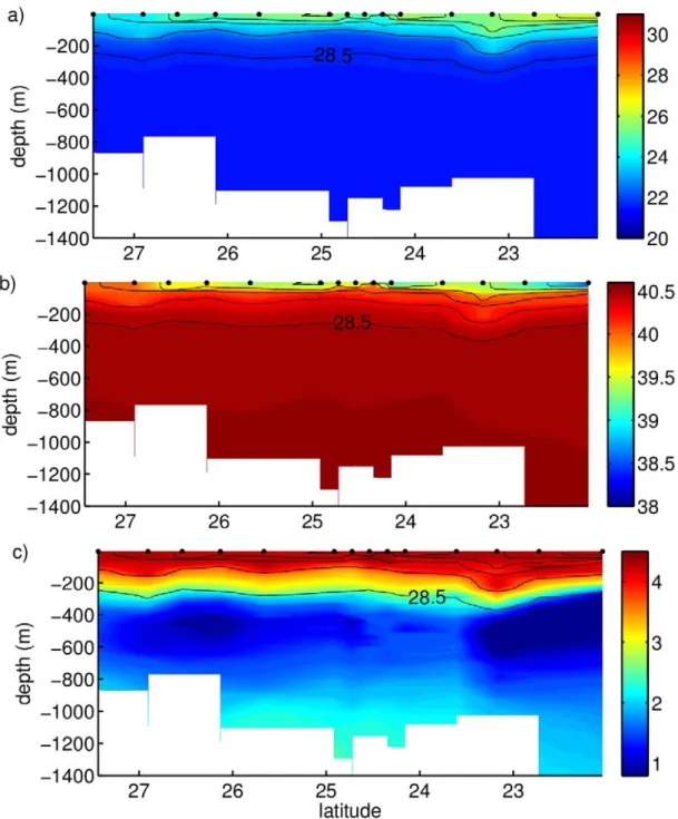
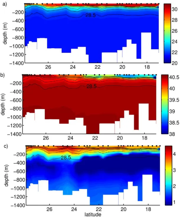
The surface salinity in the Red Sea increases from ~36.5 in the south to ~41 in the north (Cember, 1988; Sofianos and Johns, 2007). Figure 1.2 and Figure 1.3 show the distribution of water properties measured in March 2010 and September-October 2011. These figures indicate that the surface water properties display strong seasonal variations. The fresher warm water in the south and the saltier cold water in the north form a meridional density gradient at the surface.

Figure 1.2: Water properties along the central axis of the Red Sea in March 2010: (a) potential temperature (°C), (b) salinity, and (c) dissolved oxygen concentration (_mll 1_{). Black dots}

Figure 1.3: Water properties along the central axis of the Red Sea in September-October 2011: (a) potential temperature (°C), (b) salinity, and (c) dissolved oxygen concentration (_mll 1_{). Black}

1.1.2 RSOW

RSOW is one of the most saline water masses in the world ocean. It outflows into the Gulf of Aden from the Red Sea and moves southward along the African coast. Although the annual transport of RSOW through the Strait of Bab el Mandeb is only 0.36 Sv (Murray and Johns, 1997), its signal is observed in the Indian Ocean up to 6000 km away from its source as a salinity maximum at intermediate depth (Gordon et al., 1987; Valentine et al., 1993; Beal et al., 2000). In this section, unless otherwise specified, winter is defined as November through March, and summer is defined as June through September. Previous studies in the Strait of Bab el Mandeb (e.g., Morcos, 1970; Maillard and Soliman, 1986; Patzert, 1974; Neuman and McGill, 1962; Murray and Johns, 1997) indicate a 2-layer exchange flow pattern in winter and a 3-layer exchange flow pattern in summer season, as shown in Figure 1.4. In winter season, RSOW that has salinity of 40 flows out of the Red Sea beneath an incoming surface layer from the Gulf of Aden that has salinity of 36.5 psu. In summer, the exchange flow has a 3-layer structure: a surface flow from the Red Sea, the incoming Gulf of Aden Intermediate Water and, the outgoing RSOW. An 18-month time series of moored ADCP and hydrographic observations of the exchange flow at the Strait of Bab el Mandeb was collected in 1995-1996 (Murray and Johns, 1997; Sofianos et al., 2002). Velocity data indicate that in winter the average transport of RSOW is 0.6 Sv, with a speed of 0.8-1 _ms-1_{. In summer, the mean RSOW transport is reduced to 0.05 Sv, with a speed of}

0.2-0.3 _ms-1_{. Sofianos and Johns (2002) used the Miami Isopycnic Coordinate Ocean Model}

(MICOM) to study the causes of the seasonal variation of flow through the Strait of Bab el Mandeb. They argue that a combination of seasonal variations in wind stress and thermohaline forcing produces the seasonal exchange flow pattern.

Sofianos and Johns (2003) also used MICOM to suggest that RSOW is formed in the northern Red Sea through open-ocean convection. In their model, there is a cyclonic gyre in the northern Red Sea, which is an important precondition for open-ocean convection (Marshall and Scott., 1999). The cyclonic gyre brings water from the deeper ocean to the surface, with weak stratification. In winter, convection starts when the weakly stratified water is exposed to surface cooling. The cyclonic gyre in the northern Red Sea has been observed by Morcos and Soliman (1972), Clifford et al. (1997), and Manasrah et al. (2004). Trajectories of five surface drifters during 1993–1994 showed a cyclonic gyre north of 26°N ( Clifford et al., 1997).

Figure 1.4: Sketch of the two circulation patterns in the Strait of Bab el Mandeb. Left: winter, Right: summer. SW = surface water, GAIW = Gulf of Aden Intermediate Water, RSOW = Red Sea Overflow Water, SBM = Strait of Bab el Mandeb, and GA = Gulf of Aden (reproduced from Smeed, 2004, his Fig. 1).

1.1.3 GAIW

Figure 1.4 shows that GAIW flows into the Red Sea in summer. GAIW is fresher and colder than ambient surface water and RSOW. Observations made in April –December 1996 in the Strait of Bab el Mandeb show that the salinity of GAIW is as low as 36.2 and the temperature is about 18°C (Murray and Johns, 1997). Hydrographic data collected in August 2001 in the Strait of Bab

el Mandeb near the Hanish Sill confirm the GAIW characteristics of relatively low salinity, low temperature, and low oxygen concentration (Sofianos and Johns, 2007).

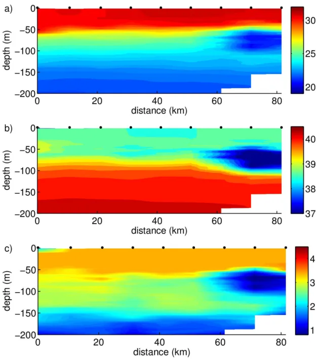
Analysis of ADCP data near the Hanish Sill and Perim Narrows from June 1995 through November 1996 reveals that GAIW transport reaches its maximum value of 0.3 Sv in summer (Sofianos et al., 2002). Sofianos and Johns (2007) analyzed hydrographic data collected in the Red Sea in August 2001. They found that GAIW can be traced northward in the Red Sea to 22°N. GAIW was also observed in September-October 2011 in the Red Sea (Churchill et al., submitted). Figure 1.3 and Figure 1.5 clearly show that GAIW is characterized by low temperature, salinity and oxygen values at the southern end of the section along the central axis of the Red Sea. This survey showed that GAIW was flowing near the eastern boundary after it enters the Red Sea.

Figure 1.5: Red Sea water properties measured in September-October 2011 along transect 2 (transect location is shown in Figure 1.6): (a) potential temperature (°C), (b) salinity, and (c) dissolved oxygen concentration (_mll 1_{). Black dots indicate station locations. Distance (km) is}

Figure 1.6: Location of transect 2, September-October 2011.

1.1.4 RSDW

RSDW, which underlies RSOW, is a nearly homogeneous water mass that fills the Red Sea basin from a depth of about 200 m to the bottom. Figure 1.2 and Figure 1.3 shows that RSDW is nearly homogeneous in salinity (40.6-40.8) and potential temperature (21-21.5 °C). The typical potential density of RSDW is 1028.55-1028.63 _kgm-3_{. The Hanish Sill depth is 137 m, which is shallower}

than RSDW. Therefore, RSDW might not be able to flow over the sill into the Gulf of Aden. Historic hydrographic data suggest that the Gulf of Suez outflow water is likely to be the main source of RSDW, while the overflow water from Gulf of Aqaba might be a secondary source of RSDW (Cember, 1988). By analyzing current measurements at the mouth of the Gulf of Suez during late winter 1971-1972, Maillard (1974) found that the wintertime outflow transport from the Gulf of Suez is 0.082 Sv. Data from 12 moored current meters in the Tiran Strait, which

connects the Gulf of Aqaba and the Red Sea, indicated that the overflow transport from the Gulf of Aqaba to the Red Sea was about 0.029 Sv in February 1982 (Murray et al., 1984). However, these data were collected over a short time period and therefore may not be representative of the annual mean. Biton and Gildor (2011) used the MIT general circulation model (MITgcm) to simulate the circulation in Gulf of Aqaba and the exchange flow between the Gulf of Aqaba and the northern Red Sea. They estimated that the annual mean outflow from the Gulf of Aqaba to the northern Red Sea is 0.0185 Sv, with a flow of 0.04 Sv during early winter and 0.005 Sv during early spring.

Natural and anthropogenic tracers, such as 3He, 14C, and chlorofluorocarbons (CFCs), are frequently used in ocean circulation studies to define the pathways, timescales, and transport of deep water masses. CFCs are trace gases of industrial origin that cause stratospheric ozone depletion. Release of CFCs into the atmosphere began in the 1940s, and their concentration in the atmosphere increased with time until the 1990s, when their use was curtailed by the Montreal Protocol. A small fraction of atmospheric CFCs enters the ocean through air-sea gas exchange at the ocean surface. They are chemically inert in seawater, and are carried from the surface to the interior by currents and turbulent mixing. CFCs can be used as an indicator of ocean ventilation and to determine the source of deep water formation. CFCs have been used extensively as a tracer to study the spreading of North Atlantic Deep Water and Antarctic Bottom Water (Smethie, 1993, 2000; Schlosser et al., 1991; Willey et al., 2004).

A few CFC profiles were collected in the far northern Red Sea and the Gulf of Aqaba in February and March 1999 (Plähn et al., 2002). These profiles revealed that RSDW could be divided into deep and bottom water masses. Overflow of very dense water from Gulf of Aqaba (through the Tiran Strait) is the main source of the bottom water. Although Cember (1988)

suggested that outflow water from the Gulf of Suez is the main source of RSDW, outflow water from the Gulf of Suez is not dense enough to sink to the bottom and it reaches gravitational equilibrium above the water from the Gulf of Aqaba.

1.2 Overturning circulations in the Red Sea

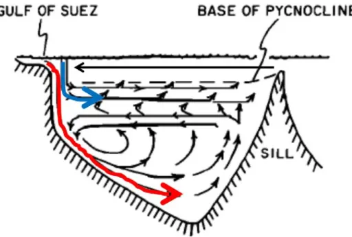
Previous studies suggest that there are two overturning circulation cells in the Red Sea, driven by open-ocean convection in the northern Red Sea and dense outflows from Gulf of Suez and Gulf of Aqaba. Figure 1.7 shows a schematic diagram of the overturning circulation in the Red Sea according to Cember (1988). The upper overturning circulation cell consists of a northward flow at the surface and a subsurface southward flow of “isopycnal mode” water. Low-salinity surface water enters the Red Sea from the Gulf of Aden. Cember (1988) suggests that the isopycnal mode water is formed mainly by open-ocean convection and then injected below the thermocline. According to Sofianos and Johns (2003), the isopycnal mode water is identified as RSOW.

The upper overturning circulation cell was also predicted by a two-dimendional similarity model developed by Phillips (1966). In his model, the Red Sea is a semi-enclosed basin with a sill on a meridional-vertical plane, and rotation is not considered. In his model, the upper overturning circulation is driven by a uniform buoyancy flux, and the sill depth marks the lower limit of the circulation, with the deeper ocean being almost motionless. Phillips’ model agrees qualitatively with the observed winter flow pattern at the Strait of Bab el Mandeb. However, later work by Tragou and Garrett (1997) and Yao et al. (2014b) found that Phillips’ similarity solution doesn’t agree well with observations and numerical simulation. Tragou and Garret (1997) modified Phillips’ model and suggested that a large eddy viscosity is required in the southward return flow in order to match the observed stratification.

Due to its elongated shape, the Red Sea is usually treated as a two-dimensional basin in early studies. However, modeling studies by Eshel and Naik (1997), Sofianos and Johns (2003), Biton et al. (2008), and Yao et al. (2014a, b) suggest that the Red Sea circulation is a more complex three-dimensional system. Sofianos and Johns (2003), and Yao et al. (2014b) studied the buoyancy driven circulation in the Red Sea and found that inflow from the Gulf of Aden moves along the western boundary and then crosses the basin to the eastern boundary. Chapter 3 of this thesis will further explore the mechanism that is responsible for the crossover of the boundary currents.

Figure 1.7 also shows a deep overturning circulation cell in the Red Sea. Dense water from the Gulf of Suez and Gulf of Aqaba sinks to the bottom of the Red Sea and moves southward. Near the sill in the southern Red Sea, it is thought that the water upwells and returns northward at a depth of about 300–500 m. As the intermediate water moves northward, it mixes with the pycnocline water. Evidence for this deep cell is found in the vertical profiles of helium-3 (3He). Figure 1.8 shows the distribution of 3He from 3 GEOSECS stations in the Red Sea (Cember, 1988). The three stations were located along the central axis of the Red Sea at 14.7°N, 19.9°N, and 27.3°N, and each had a maximum 3_{He concentration at about 500 m. The} 3_{He concentration}

increases southward near the bottom.

In seawater, 3_{He in has two sources: air-sea exchange and Earth’s interior. Cember pointed out}

that most of the 3He is released from Earth’s interior by tectonic activity. The 3He distribution shown in Figure 1.8 suggests that the deep water moves southward and gathers 3He, which is released from the sea floor. At the southernmost Red Sea (near the Hanish Sill), the deep water is supposedly uplifted along the topography and reaches its maximum concentration of 3_{He at about}

distance from the source and vertical mixing with ambient water, which has a low 3He concentration.

Cember’s hypothesis of the deep overturning circulation is based on data from only three stations in the Red Sea. Dissolved oxygen and CFC-12 can also be used as indicators of the deep overturning circulation. At the bottom in the northern Red Sea, high dissolved-oxygen concentrations were observed, indicating newly formed deep water. When RSDW moves southward, the dissolved oxygen is depleted, and its concentration decreases (Sofianos and Johns, 2007). The dissolved-oxygen minimum occurs at about 400 m, which could be an indication of relatively old recirculating deep water flowing northward. Although there is no direct measurement of the intermediate northward return flow, the distribution of carbon-14, 3He, and oxygen is consistent with its existence (Cember, 1988; Sofianos and Johns, 2007).

Figure 1.7: Schematic of general circulation in the Red Sea, according to Cember (1988, his Fig. 1). The red and blue arrows indicate convective and isopycnal modes, respectively.

Figure 1.8: Distribution of 3He in the Red Sea (Cember, 1988; his Fig. 7). 1.3 Thesis Outline

This study focuses on the upper overturning circulation cell, which is primarily driven by surface buoyancy loss. The upper overturning circulation cell connects the Red Sea with the open ocean and governs exchange processes between the Red Sea and the Indian Ocean. Fresher water coming from the Indian Ocean undergoes heat loss and evaporation in the Red Sea and is transformed into saltier RSOW. Based on results from a numerical study, Sofianos and Johns (2003) suggest that RSOW is formed by open-ocean convection in the northern Red Sea. In Chapter 2 of this work, new observations are analyzed to support the hypothesis that RSOW is

formed by open-ocean convection and to identify RSOW. Numerical modeling is used to study the pathways and transit time of RSOW from its origin to the Strait of Bab el Mandeb.

Buoyancy-loss forced circulation in marginal seas is usually dominated by cyclonic boundary currents (Spall, 2004). However, a numerical studies by Sofianos and Johns (2003) and Yao et al. (2014b) indicate that the Red Sea circulation is more complex, with a cyclonic gyre in the northern Red Sea and an anticyclonic gyre in the southern Red Sea. They found from their numerical simulations that the northward boundary current crosses the basin from the western boundary to the eastern boundary at a certain latitude (crossover latitude). Sofianos and Johns (2003) suggested that the crossover latitude is the latitude beyond which Rossby waves are no longer possible. Numerical experiments in Chapter 3 show that their explanation cannot be correct. A new mechanism for the crossover of boundary currents is studied in Chapter 3, using numerical modeling and an ad hoc analytical model.

Some observational and modeling studies have shown that the surface-layer circulation in the Red Sea is characterized by a series of basin-scale eddies (Morcos, 1970; Morcos and Soliman, 1972; Quadfasel and Baudner, 1993). The cyclonic and anticyclonic gyres are not permanent, but tend to reappear at preferential locations, such as the anticyclonic eddy centered at 23°N and the cyclonic eddy near 26°N. These eddies are strong and are usually confined to the upper 100-200 m. Using shipboard ADCP, Sofianos and Johns (2007) observed a strong dipole near 19°N in August 2001, with a cyclone to the north and an anticyclone to the south, both with a maximum speed of about _1ms-1_{. These eddies can influence the distribution of water properties, such as}

chlorophyll concentrations. On the other hand, water properties can be used as an indicator of eddies. For example, the distribution of chlorophyll-a from SeaWiFS indicates an anticyclone

centered at 23°N in August 1998 and an anticyclone centered at 18.7°N in October 2002 (Acker et al., 2007).

Eddies play an important role in transporting heat, freshwater, and mass in the Red Sea. However, the mechanisms that generate these eddies are not well-understood. Clifford et al. (1997) suggested that cross-basin wind fields can generate eddies in the Red Sea. Zhai and Bower (2013) studied the Red Sea response to the Tokar Wind Jet which blows eastward from Sudan onto the Red Sea. They found that the Tokar Wind Jet generates a dipole, i.e. two counter-rotating eddies. In Chapter 4, the eddy generation mechanism that is related to cross-basin winds is reviewed. Chapter 4 also studies two additional mechanisms for eddy generation in the Red Sea: baroclinic instability, and meridional structure of surface buoyancy forcing.

Chapter 2

Red Sea Overflow Water Formation and its Spreading Pathways

2.1 Introduction and background

RSOW is one of the most saline water masses in the world ocean. After flowing over the Hanish Sill, the RSOW entrains less dense overlying water in the Gulf of Aden and its properties changes dramatically. With a combination of observational data and numerical simulations, Bower et al. (2000, 2005) found that the RSOW reached neutral buoyancy at about 400-800 m in the Gulf of Aden with salinity of 37.5. Outside the Gulf of Aden, the RSOW has been observed up to 6000 km away from its source in the Agulhas retroflection region as a water mass with high salinity and low oxygen at intermediate depth (Gordon et al., 1987; Valentine et al., 1993; Beal et al., 2000). It has been observed that the primary spreading pathway of RSOW is along the African continental coast through the Mozambique Channel (Wyrtki, 1973; Beal et al., 2000). By using a simple mixing model, Beal et al. (2000) suggested that RSOW dominated the Indian Ocean salt budget in the intermediate depth layer. The RSOW can also be used as a tracer to investigate the Indian Ocean circulation. The RSOW is suggested to be formed in the northern Red Sea through open-ocean convection. Atmospheric conditions there directly influences production rate of RSOW. Therefore, understanding the formation mechanism of RSOW and how RSOW production rate changes under difference conditions in the Red Sea is important in studying the RSOW’s impact on Indian Ocean circulation and properties.

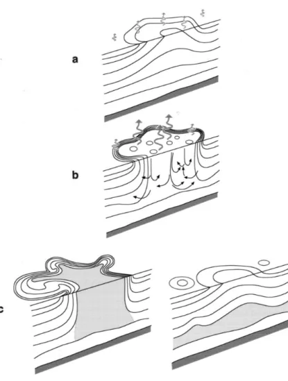
important processes by which the intermediate and deep water masses in the global oceans are formed. The Labrador, Greenland, Mediterranean and Weddell Seas are major open-ocean convection locations. Intermediate or deep water masses formed in these convective regions usually hold distinct water properties which allow them to be tracked far from their origins. The evolution of open-ocean convection can be divided into the three phases shown in Figure 2.1: preconditioning, deep convection, lateral exchange and spreading. Open-ocean convection can occur when three conditions are satisfied: i) the water column is weakly stratified; ii) the cyclonic gyre with doming isopycnals brings the denser deep water close to the sea surface; iii) there is intense sea surface buoyancy loss to the atmosphere due to cooling and evaporation (Marshall and Schott, 1999). When these conditions are satisfied, vigorous vertical mixing occurs within the preconditioned area (Figure 2.1b). At the same time, eddy flux spreads the homogeneous water column horizontally. When the surface buoyancy loss decreases or ceases, the surface water becomes restratified. A well-mixed layer remains as intermediate or deep water (right panel of Figure 2.1c) below the surface (Marshall and Schott, 1999) and spreads out at its neutrally buoyant level.

Figure 2.1: A schematic diagram of the three phases of open-ocean convection: (a) precondition, (b) deep convection, (c) lateral exchange and spreading. The curly arrows represent surface buoyancy loss and the shaded is the water mixed by convection. (Marshall and Schott, 1999, their Figure 3).

Hence, preconditioning is an essential prerequisite for open-ocean convection. Marshall and Schott (1999) summarized the preconditions of open-ocean convection in the North Atlantic and West Mediterranean. Cyclonic boundary circulations are observed in the Labrador, Greenland and West Mediterranean Seas where deep convection also occurs. For example, in the Labrador Sea, the cyclonic circulation is composed of the West Greenland Current and the Labrador

remove heat and fresh water from the sea surface. In the Greenland Sea, brine rejection from ice also plays an important role in surface density increase. The typical values of net heat fluxes from ocean to atmosphere in winter in the Labrador, Greenland and Mediterranean Seas are -490, -530 and -500 _{W m}2_{, respectively (Marshall and Schott, 1999). Based on CFC-11 inventories,}

Smethie and Fine (2001) estimated the deep water formation rates: 7.4 Sv for Labrador Sea Water, 2.4 Sv for Denmark Strait Overflow Water, and 5.2 Sv for Iceland-Scotland Overflow Water. The transport of the Mediterranean Overflow Water is about 1 Sv at the Strait of Gibraltar according to observations (Send et al., 1999).

The primary aim of this chapter is to understand the formation process of the RSOW and the three-dimensional spreading pathways in the Red Sea. Section 2.2 introduces the data sets used in this study. The preconditioning of open-ocean convection in the northern Red Sea is described in Section 2.3. In Section 2.4, potential vorticity and chlorofluorocarbon-12 (CFC-12) distributions are used to identify the RSOW. In Section 2.5 the production rate of the RSOW is estimated using a method developed by Walin (1982). The spreading pathways and transit time of the RSOW calculated from a numerical model will be described in Section 2.6. Section 2.7 contains conclusions and a discussion of this chapter.

2.2 Data

2.2.1 Hydrographic and CFC-12 data

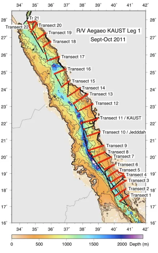
Two hydrographic survey cruises were conducted in the Red Sea during March 16-29, 2010 and September 15-October 10, 2011 by the Woods Hole Oceanographic Institution and King Abdullah University of Science and Technology. The primary purpose of these cruises was to carry out a large-scale survey of the eastern Red Sea, including observations of top-to-bottom

ocean currents and water properties, including temperature, salinity, dissolved oxygen, turbidity and fluorescence. The cruise that was conducted in March 2010 consisted of 111 CTD (Conductivity, Temperature, and Depth) and LADCP (Lowered Acoustic Doppler Current Profiler) stations. The cruise in September and October 2011 consisted of 206 CTD and LADCP stations. Figure 2.2 shows the locations of CTD and LADCP stations for these two cruises. The station spacing along each transect was about 10 km. At each station, profiles of temperature, salinity, dissolved oxygen and velocity data were collected using a modified SeaBird 911plus rosette/CTD system and LADCP. Seawater samples were collected at nearly all stations to calibrate CTD measurements of salinity and oxygen. Velocity in the upper 600 meters was measured by Shipboard ADCP.

Figure 2.2: Locations of CTD stations of Red Sea cruise in March 2010 and September-October 2011 (Bower, 2010; Bower and Abualnaja, 2011).

During the September-October 2011 Red Sea cruise, water samples for CFC-12 analysis were collected at selected stations. The locations where CFC-12 samples were collected are shown in Figure 2.3. Water samples were collected by using two methods. 250 ml stoppered bottles were used to collect samples for CFC-12 at 5 stations. 50 ml ampoules were used to collect CFC-12 samples at 14 stations. Nitrogen was used to flow through the top of the ampoules to keep the water samples from being contaminated by air. The flame-sealing of the glass ampoule samples was done by propane and oxygen. Both stoppered bottles and ampoules samples were collected at stations 194, 157 and 205 in order to compare the two sampling methods and increase the measurement accuracy. The CFC-12 data obtained during the 2011 cruise were the first data for the Red Sea that covers from 17°N to 28°N.

Figure 2.3: Station numbers and locations for CFC-12 water sample collection during September 15-October 10, 2011 Red Sea cruise.

2.2.2 Sea Surface Temperature

SSTs can be determined from satellite remote sensing using microwave (MW) and infrared (IR) radiometers. IR SSTs have higher spatial resolution (1-4 km) than MW SSTs (25 km) does. However, the accuracy of IR SSTs is affected by cloud, aerosols and water vapors. The advantage of MW radiometry is that it is not affected by cloud cover. In this study we use MW-IR SSTs which is processed and distributed by Remote Sensing System (RSS). This product combines the satellite observations from MW and IR sensors. The MW SSTs are derived from

Mission’s Microwave Image (TMI) and the WindSAT Polarimetric Radiometer (WindSAT). The IR SSTs are derived from MODerate-resolution Imaging Spectroradiometer (MODIS). The merged MW-IR SST product has greater coverage and higher resolution. This product is distributed on a 0.09° grid and covers data from January 2006.

2.2.3 Sea Surface Heat Flux

The sea surface heat flux used in estimating the production rate of RSOW is obtained from the global Objectively Analyzed air-sea Flux (OAflux). The OAflux is constructed from an objective analysis of in situ observations, satellite data and atmospheric reanalysis (Yu et al., 2008). The fluxes are computed using the Coupled Ocean-Atmosphere Response Experiment (COARE) bulk flux algorithm 3.0 and are mapped on a regular 1° grid. The data product used in this study includes the monthly mean net heat flux and evaporation for the period from 1984 to 2009. 2.2.4 QuikSCAT and ASCAT Winds

The QuikSCAT was launched in 1999 and its mission ended in November 2009. The QuikSCAT (Quik SCATterometer) winds analyzed here are produced by Remote Sensing Systems and sponsored by the NASA Ocean Vector Winds Science Team. QuikSCAT data product includes daily and time averaged wind data (3-day average, weekly and monthly) at 10 m above the sea surface. The data product used here is 0.25-degree gridded data. An air-sea interaction buoy was deployed on October 11, 2008 at 22.16°N, 38.50°E in the Red Sea 60 km offshore of the Saudi Arabian coast. The QuikSCAT wind speeds compare well with the buoy wind measurements (Zhai and Bower, 2013). Their results show that the mean differences for wind speed and

direction are -0.02 _ms-1 _{and 10.7°, root mean squared differences are 0.68 ms}-1 _{and 29.9° and}

correlation coefficients of 0.95 and 0.76.

The Advanced Scatterometer (ASCAT) on board Metop-A was launched in 2006 and provides sea surface wind at 10 m height since March 2007. The data product is mapped on a 0.25 degree grid. ASCAT wind has similar accuracies to QuikSCAT based on previous studies (Bentamy et al., 2008). Wind data before November 2009 used in this study are from QuikSCAT and data after November 2009 are from ASCAT.

2.3 Preconditioning of Open- Ocean Convection in the Northern Red Sea

Open-ocean convection can reach thousands of meters in the North Atlantic region. However, the situation in the northern Red Sea is different. In order to escape to the Gulf of Aden, RSOW formed in the northern Red Sea has to flow over the Hanish Sill with a depth of 137 m. Therefore, convection down to this depth is sufficient for the formation of the RSOW.

Observations in the Labrador, Greenland and Mediterranean Seas suggest that open-ocean convection occurs in open-ocean regions that are close to boundaries because wind blowing from land usually brings cold and dry air which can remove sensible heat, latent heat and fresh water from the sea surface. Although the Red Sea region is not as cold as high latitudes, the air here is exceptionally dry, leading to strong evaporation and latent heat loss. In addition to the intense atmospheric forcing, two more features are usually observed in open-ocean convection region: weak stratification and cyclonic gyre (Marshall and Schott, 1999). Cyclonic circulation can cause doming of isopycnal surfaces and raise the weakly-stratified water to the surface. In this section,

Some previous observations in the Red Sea suggest that there is a cyclonic gyre in the northern Red Sea (Morcos and Soliman, 1974; Clifford et al., 1997; and Manasrah, 2004; Chen et al., 2014). The cyclonic gyre is also suggested in satellite SST images. Figure 2.4 shows the monthly mean SST anomaly in March, June, October and December. Monthly mean SST is obtained by averaging MW-IR SST from January 2006 to December 2012. The SST anomaly is obtained by subtracting the spatial average of monthly mean SST of each month in the area north of 22°N from monthly mean SST. It is obvious that there is a cold pool in the northern Red Sea in October and December. Cold pool is usually associated with lower sea level, which suggests the emergence of a cyclonic gyre. The center of the cold pool is closer to the western part of the basin. The SST images also suggest that the closed contours disappear on the western boundary in March and June, which eliminates evidence of a closed cyclonic gyre.

Figure 2.4: Monthly mean SST anomaly for March, June, October and December. Here anomaly means that spatial average of SST is subtracted for each month. The contour interval is 0.2 °C, and thick black line is zero-contour.

Although in situ observations are sparse, several investigators have found evidence of cyclonic circulation in the northern Red Sea (Morcos and Soliman, 1972; Clifford et al., 1997; Manasrah et al., 2004). Potential density at Transects 18, 19 and 20 in the northern Red Sea in October

2011 cruise are plotted in Figure 2.5. It indicates a shoaling of isopycnals toward the interior of the basin, consistent with a cyclonic gyre there. However, we were not able to capture the structure of the western part of the cyclonic gyre due to political reasons. Sofianos and Johns (2007) described zonal sections of temperature, salinity, oxygen and velocity on the western half of the Red Sea at about 26.5°N in August 2001. The western half of the cyclonic gyre was captured by their observations, with a southward flow along the western boundary and eastward rising isopycnals.

Figure 2.5: Potential density at Transects 18, 19 and 20 in September-October 2011 cruise (See Figure 2.2 for location). x-axis is distance from the most west station. Isopycnals of 27.5, 28 and 28.5 kg m-3 are plotted with black lines.

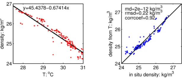
The SST images exhibit that the coldest water in winter (December to February) is located closer to the western part of the basin than the eastern part. Since satellite sea surface salinity (SSS) is not available in the Red Sea, surface density can’t be calculated directly from remotely measured surface temperature and salinity. The scatter plot of surface temperature and density measured during March 2010 cruise reveals that the surface density was linearly related to the SST (Figure 2.6). The least square fit of the linear relation between SST and density is

SST 0.61571 42.2302  

 _{(Figure 2.6). Here 0.67414 is not a thermal expansion coefficient} since the salinity part of the equation of state is included implicitly. Density can be approximated by a linear equation of state, such that density is linearly related to salinity and temperature. Figure 2.7 shows that salinity is also linearly related to SST in the north Red Sea. Therefore, there is a very close agreement between the density calculated from in situ salinity and temperature (in situ density) and the density estimated from in situ temperature. The statistical analysis reveals that the linear correlation coefficient is 0.99 with a mean difference and root mean squared difference of _21012_kgm3 _{and 0.06 kgm}3 _{, respectively (Figure 2.6). By}

employing the linear relation between density and SST, we can estimate density and explore its horizontal structure. I am assuming that the linear relationship observed in March 2010 holds throughout the winter months. Figure 2.9 shows sea surface density in December, January and February calculated from satellite SST. It implies that there is a cyclonic gyre in December and January. The cyclonic gyre disappears in February because convection might stop in February and water column gets restratified. The densest water is located closer to the western part of the basin. In situ observations at the strait of Bab el Mandeb recorded that the density of the RSOW at the strait was about 27.5~28 _kgm3 _{(Sofianos et al., 2002). As shown in Figure 2.9, the 27.5}

kg/m3 isopycnal outcrops in January and February in the northern Red Sea, which makes it possible for the RSOW formation. It should be pointed out that the linear relation between SST and density is based on the in situ observation during March 2010 cruise. The least square fit of the linear relation between SST and density for September-October 2011 cruise was

SST 0.67414 45.4378  

 _{(Figure 2.8), which was very close to the linear relation in March} 2010. The root mean squared difference of the in situ density and density calculated from temperature is 0.22 3

m

the linear relation between SST and



Figure 2.6: Left: Relationship between surface temperature and density in the northern Red Sea (north of 22 °N). Red dots represent temperature and density observed during March 2010 cruise in the upper 5 meters. Black line is least square fit of the linear relation between temperature and density. Right: Comparison between the density calculated from in situ temperature and salinity (x-axis) and density calculated using the linear relation between temperature and density shown in the left panel (y-axis).

Figure 2.7: Relationship between surface temperature and salinity in the northern Red Sea (north of 22°N). Red dots are temperature and salinity observed during March 2010 cruise in the upper 5 meters. Black line is least square fit of the linear relation between temperature and salinity.

Figure 2.8: The same as Figure 2.6, but data are from September-October 2011 cruise.

Figure 2.9: Sea surface density in December, January and February calculated from satellite SST through the linear relation based on observation during March 2010 cruise. The contour interval is 0.2 kg/m3. The thick black line represents the 27.5 kg m-3 isopycnal.

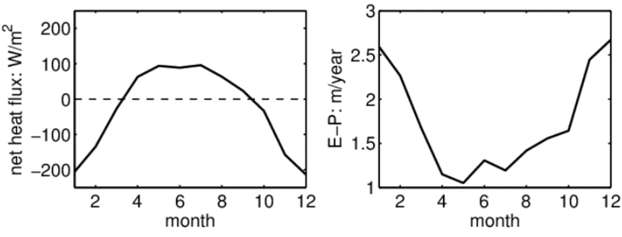
The seasonal cycle of net heat flux and evaporation rate averaged north of 25°N are plotted in Figure 2.10. In summer, the net heat flux is positive, which means that the sea surface gains heat from the atmosphere. Starting from September, the net heat flux changes its sign and the sea surface begins to lose heat into the atmosphere. In December and January, the heat loss

approaches -200 W m-2, which is much smaller than the heat loss in Labrador (-490 W m-2), Greenland (-530 W m-2_{) and Mediterranean (-500 W m}-2_{) Seas. However, as we have mentioned}

earlier, the convection doesn’t have to be deeper than 200 m in the northern Red Sea because the RSOW flows over a sill with a depth of 137 m. Papadopoulos et al. (2013) found that the net heat loss in winter in the northern Red Sea varied from -50 W m-2 to -400 W m-2 from year to year. They pointed out that the extreme heat loss events in certain years were caused by positive sea level pressure (SLP) anomaly over the eastern Mediterranean and Middle East. In these years, the strong southeastward wind carried cold and dry air into the northern Red Sea and led to extreme heat loss and evaporation.

Figure 2.10: Annual mean net heat flux and evaporation rate averaged north of 25°N.

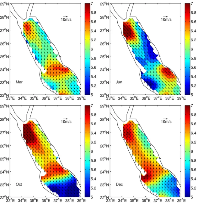
Figure 2.4 and Figure 2.9 reveals that the coldest and densest water is located closer to the western part of the basin instead of being in the middle of the northern Red Sea. The horizontal structure of surface 10-m winds shows that the winds are stronger near the western boundary than that near the eastern boundary (Figure 2.11). Gulfs of Suez and Gulf of Aqaba connect with the northern Red Sea and are surrounded by mountains. The surface winds in the two gulfs are mainly along the longitudinal axis of the basins due to the mountains’ constraint. Winds from the

Gulf of Suez and Gulf of Aqaba converge near the western boundary of the northern Red Sea and cause stronger wind there. This idea is supported by a high resolution numerical simulation using the Weather Research and Forecasting (WRF) model (Jiang et al., 2009). Their simulation captured the wind pattern in the Gulf of Suez and Gulf of Aqaba, which was not observed by QuikSCAT. The turbulent heat flux (including latent and sensible heat fluxes) and evaporation increase with wind speed. Therefore, wind can influence the surface temperature and salinity. The presence of stronger winds close to the western boundary might explain the asymmetry in the cold pool.

Figure 2.11: Monthly mean of 10-m wind vector field overlapped with its magnitude (color contours) from QuikSCAT.

In summary, there is evidence to support a cyclonic gyre with doming isopycnals in the center of the northern Red Sea from satellite SST and hydrographic data. This study also indicates that the cyclonic gyre is closer to the western boundary. In winter, strong buoyancy loss causes vertical mixing in the weakly stratified layer and convection occurs. The preconditions of open-ocean

convection are satisfied in the northern Red Sea. Figure 2.1c shows that there is a nearly homogeneous water layer that remains below the sea surface after convection ceases. This water mass is usually marked with distinct properties, such as low potential vorticity (PV) and high oxygen. Only a few studies have addressed the southward spreading of RSOW after its formation (Phillips, 1966; Cember 1988; Sofianos and Johns, 2003). Phillips (1966) developed a 2-dimention similarity model to study buoyancy-driven circulation in the Red Sea. He pointed out that buoyancy loss over the Red Sea surface drives a shallow overturning circulation which included a northward surface current and a southward subsurface current. The southward flow returns to the Gulf of Aden and is known as RSOW. Based on Carbon-14 and 3He profiles at three stations along the middle axis of the Red Sea, Cember (1988) identified a southward-flowing current in about 100-200 m depth range. Sofianos and Johns (2003) simulated the formation and spreading of RSOW using the Miami Isopycnic Coordinate Ocean Model (MICOM). They found that RSOW was carried out of the Red Sea by a southward undercurrent after RSOW was formed in the northern Red Sea. These studies of southward spreading of RSOW are based on limited observations or numerical simulations. This study will provide new evidence to explore the southward spreading of the RSOW by analyzing hydrographic data, CFC-12 data and numerical output in the following sections.

2.4 Observations of the RSOW in the Red Sea

In the last section, it was shown that the northern Red Sea is preconditioned for open-ocean convection. When convection stops and the surface water starts to restratify, the recently formed RSOW with nearly homogeneous water properties remains trapped below surface and flows southward in a specific density range. The homogeneous layer signifies weak stratification and

thus relatively low potential vorticity ( z f    

₀ ). Figure 2.12 shows potential vorticity calculated from density profiles measured in March 2010 cruise. The RSOW is identifiable by a minimum of potential vorticity which is bounded by isopycnals of 27.5 and 27.8 -3

m

kg . Isopycnal of 27.5

-3

m

kg outcrops at transect 1 and 2 where open-ocean convection could have occurred. The distribution of the minimum of potential vorticity layer compares well with the two bounded isopycnals. For example, at transect 7, the two isopycnals rise eastward in the same direction as the minimum of potential vorticity layer. The deeper low PV layer is associated with RSDW.

Figure 2.12: Potential vorticity (_m1_s1_{) at nine transects during March 2010 cruise (See Figure}

2.2 for location). x-axis is distance from the most west station. Isopycnals of 27.5 and 27.8

-3

m

kg are plotted. Distance (km) is from the west side of the transec.

The minimum of potential vorticity layer is also observed in September-October 2011 cruise (Figure 2.13). In addition to potential vorticity, chemically inert tracers, such as CFC-12 can also

be used to trace and identify water masses. Water samples of CFC-12 were collected at 16 stations during September-October 2011 cruise by using either stoppered bottles or ampoules and then measured by Smethie’s lab at Lamont-Doherty Earth Observatory. At three stations, both methods were used to collect CFC-12 water samples. Figure 2.14 plots the vertical profile of CFC-12 at these three stations. Measurements by the two methods generally agree well with each other, with mean difference of 0.004 _pmolkg-1_{. The coefficient of variation of the root mean}

squared deviation between the two methods is 0.0297. In Figure 2.14, there is a maximum of CFC-12 layer centered at about 150 m depth and a minimum of CFC layer centered at about 400 m depth. This structure is further supported by CFC-12 measurements at other stations (Figure 2.16 and Figure 2.17). The vertical profiles of Δ14C plotted by Cember (1988) exhibits the same vertical structure (Figure 2.15) with a maximum of Δ14C layer at 100-200 m depth and a minimum of Δ14C layer at 400-600 m. The maximum of CFC-12 layer centered at 150 m depth is RSOW which is formed in the northern Red Sea by open-ocean convection. CFC-12 concentration continuously decreases from 200 m to 400 m depth and then increases till bottom. CFC-12 enters into seawater from atmosphere through the sea surface. According to our observations in March 2010 and September-October 2011 cruises, the convection in the northern Red Sea is not deep enough to replenish CFC-12 at the bottom layer. Therefore, there must be other sources that account for the relatively high CFC-12 concentration near bottom. By analyzing hydrographic and CFC-12 data measured in the Gulf of Aqaba and the northern Red Sea, Plähn et al. (2002) discussed that the sources of the Red Sea Deep Water (RSDW) include outflow water from the Gulf of Aqaba and Gulf of Suez. They suggested that the outflow from the Gulf of Aqaba is dense enough to sink to the bottom of the Red Sea, while the outflow from

the Gulf of Suez is lighter than that from the Gulf of Aqaba and overlies on top of Gulf of Aqaba water.

Figure 2.13: Potential vorticity (_m1_s1_{) at three selected transects during September-October}

2011 cruise (See Figure 2.2 for location). x-axis is distance from the most west station. Isopycnals of 27.5 and 28.1 _kgm-3 _{are plotted.}

Figure 2.14: Vertical profiles of CFC-12 at three stations. Samples collected using stoppered bottles are plotted with blue-dotted lines, while samples collected using ampoules are plotted with red-circle lines.

Figure 2.15: Vertical profiles of Δ14C from three stations in the Red Sea (Cember 1988, his Fig. 8). The station locations of 405, 407 and 408 are (34°31'E, 27°16'N), (38°30'E, 19°56'N), (42°10'E, 14°43'N), respectively.

Figure 2.16: CFC-12 concentration (pmol kg-1) along the middle axis of the Red Sea (See Figure 2.3 for location). Station numbers and depth at which measurements were taken are marked with black dots. Isopycnals of 27.5 and 28.1 _kgm-3 _{are plotted.}

Figure 2.17: The same as Figure 2.16, except that stations are closer to the eastern coast instead of along the middle axis of the Red Sea (See Figure 2.3 for location). Isopycnals of 27.5 and 28.1

-3

m

kg are plotted.

In Figure 2.16 and Figure 2.17, isopycnals of 27.5 and 28.1 _kgm-3 _{are plotted. The layer with}

maximum of CFC-12 resides in this density range, which is the same as the density range of low potential vorticity layer shown in Figure 2.13. The tongue of high CFC-12 centered at 150 m extends southward from the northern Red Sea. The concentration of CFC-12 decreases in the southward direction. This might be caused by that CFC-12 in the southern part experiences longer time mixing with ambient water, which dilutes the concentration of CFC-12. As will be suggested in Chapter 3, the path of the southward movement of RSOW may be more complex than a simple, along-axis flow. Variation of CFC-12 concentration along the section shown in Figure 2.16 and Figure 2.17 would be influenced by the circulation. Even if the path were

diffusion. It seems that the layer with high CFC-12 terminates at station 123 (Figure 2.17). This might not represent the real situation, since there is no measurement between surface and 250 m at station 123. As a result, the maximum of CFC-12 concentration might not be captured in Figure 2.17 at station 123. The distributions of potential vorticity and CFC-12 provide evidences that the RSOW is formed through open-ocean convection in the northern Red Sea and then spreads southward.

Density ranges of the RSOW chosen from 2010 cruise and 2011 cruise are different (Figure 2.12 and Figure 2.13). The densities of the minimum potential vorticity layer observed in the 2011 cruise are about 0.3 -3

m

kg higher than that in the 2010 cruise. It implies that the RSOW formed in 2011 is denser than in 2010. The mean winter surface temperature in the northern Red Sea in 2011 is about 0.6 °C colder than that in 2010 (Figure 2.18). If the relation between density and surface temperature shown in Figure 2.6 holds for winter, then sea surface density in winter 2011 is about _0.37kgm-3 _{higher than that in winter 2010. Northwesterly wind in the northern Red}

Sea brings cold and dry air from land to the Red Sea. Higher wind speed also removes more heat and freshwater from the sea surface. Figure 2.18 shows that the 10-m wind speed in winter (January, February and March) 2011 is 1.5 _ms-1 _{higher than in winter 2010. Therefore, stronger}

Figure 2.18: SST (left panel, °C) and wind speed (right panel, m/s) difference between 2011 and 2010 winter (averaged in January, February and March).

Oxygen enters seawater through air-sea interaction as CFC-12. Different from CFC-12, the concentration of oxygen can be influenced by chemical processes and biological activities. Figure 2.19 shows dissolved oxygen concentration at three transects in the March 2010 cruise. However, the relatively higher concentration is not clearly shown at transects 3, 5 and 7. Oxygen is not a conservative tracer. Therefore, dissolved oxygen might not be used as an appropriate tracer to track water masses. Comparison between oxygen and CFC-12 distributions reveals the advantage of CFC-12 as a passive tracer in identifying RSOW.

Figure 2.19: Dissolved oxygen (_mll 1_{) at selected three transects during the 2010 cruise (See}

Figure 2.2 for location). x-axis is distance from the most west station. Isopycnals of 27.5 and 27.8 _kgm-3 _{are plotted.}

In summary, the RSOW is identified as a layer with relatively low potential vorticity and higher concentration of CFC-12. In addition, the density range of the RSOW is about 27.5-27.8 _kgm3

in 2010 and 27.5-28.1 3

m

kg  in 2011. The interannual variability of atmospheric forcing might have caused the density difference of the RSOW formed in 2010 and 2011.

2.5 Production Rate of RSOW

By looking at the vertical profiles of Δ14C, Cember (1988) identified two different modes of water in the Red Sea: the convective mode and the isopycnal mode. The convective mode water with its origin from the Gulf of Suez and Gulf of Aqaba was a source for the Red Sea Deep and Bottom Water. The isopycnal mode water was the RSOW which flowed southward at a depth centered at 100 m. The formation rate of the isopycnal mode water was estimated to be about 0.11 Sv (Cember, 1988). In Sofianos and Johns’s model (2003), production rate of the RSOW formed by open-ocean convection in the northern Red Sea was about 0.25 Sv. Walin (1982) derived a theory for how water masses were transformed from one temperature class to another

by air-sea heat flux and mixing. In this section, the production rate of the RSOW will be estimated through Walin’s method.

Figure 2.20 is a schematic diagram illustrating the basic idea of Walin (1982). The control volume (R) is bounded by the sea surface, bottom, one outcropping isotherm (T₀), and a fixed control surface (B). Here the control surface is essentially vertical and lies at the entrance of the strait that connects the Red Sea and the Gulf of Aden. We will initially allow the position of isotherm T₀ to vary with time, so that the volume of R can change. Water masses are transformed from one temperature class to another due to sea surface heat losses and interior mixing (eddy diffusivity). The transformation rate ( G ) of water masses at a particular temperature can be determined from heat and volume conservation for the control volume. In Walin (1982), he started his arguments with the equations of heat and volume conservation over the control volume without a detailed derivation. Hence, it was not clear whether his arguments were valid when the isotherm T₀ varied with time. In this section, we will derive Walin’s method in more detail than what was originally presented in Walin (1982).

Figure 2.20: A schematic diagram showing the transformation of water across a isotherm by air-sea heat fluxes and interior mixing.

Integrating the continuity equation  v 0 over the control volume and using the divergence theorem, the volume conservation equation can be written as

_

A

dA

n

v , where A is the surface of the control volume, v is velocity vector, n is the unit vector normal to the control surface. The surface consists of four parts, sea surface, bottom, isotherm T T0 and a fixed

control surface B. Assuming that there is a rigid-lid sea surface and no volume flux across the sea surface and bottom, the velocity at isotherm T  can be decomposed into the net velocity T₀

through the isotherm vG and the velocity of the isotherm vA . Therefore,







v _{G A} . The change of the volume of R is caused by the moving

of isotherm T  . Therefore, T₀



The net diathermal volume flux is defined as



    0 T T dA

G vG n , and the volume flux through B

is





  z(T0)

H vdz

M . Here G and M are defined positive when directed into the control volume. Therefore, the volume budget of R is given by:

G M t

V _{ }



 _{, (2.2)}

where V is the volume of R, G is the net volume flux across isotherm surface and M is the volume flux across control surface B.

The temperature equation is

 

 _{ , in which horizontal diffusivity is neglected.}

By integrating the temperature equation over the control volume and using the divergence theorem, the advection part can be written as

 

_

_







Using definition in Eq. (2.1), temperature flux across the isotherm T  can be modified as T0







and temperature flux across the fixed control surface B is





The volume integral of the temporal change of temperature can be written as

dV t T TdV t dV T t _{R R} R        







The temporal change of volume is due to the moving of the isotherm T  , therefore, T₀

t V T dV t T dV t T T T R        





The integral of the vertical diffusion term is









 is the surface heat flux and _c4.2106 _{W sC}1_m3 _{is heat}

capacity per unit volume.

Combining Eq. (2.5)-Eq. (2.8), the integral of the temperature equation (heat budget) can be written as







F  is diffusive heat flux through the isotherm T  . T₀

0

T is not specifically chosen in the derivations above, so Eq. (2.9) is valid for any T. The heat

budget equation of R can also be written in temperature space as:







Taking partial derivative with respect to T of Eqs (2.2) and (2.10), we obtain:

T G m t       _(2.11)

T Q T F cG T G cT cmT t cT              _{. (2.12)}

Multiplying Eq. (2.11) with cT and subtracting from Eq. (2.12), the transformation rate can be

obtained by T F T Q cG        . (2.13)

Eq. (2.13) shows that the transformation rate can be determined by two processes: the one due to surface heat loss

T Q

 

 and the other one due to diffusion

T F

 

 . By neglecting the diffusive part, Walin (1982) estimated the surface North Atlantic poleward transport to be about 10 Sv. In this calculation, the diffusive part

T F

 

 in Eq. (2.13) is also neglected. If we choose two isotherm surfaces T T₁ and T T₂ as two boundaries of R , transformation rate G(T₁) and G(T₂) induced by surface heat flux can be estimated through the first term on the right-hand side of Eq. (2.13). If the upper and lower temperature limits of the RSOW are chosen as two isotherm surfaces, in a steady state, the production rate of RSOW (M ) can be estimated through the transformation rate difference between G(T₁) and G(T₂) according to Eq. (2.2). The transformation rate due to surface heat loss obtained through Eq. (2.13) is plotted in Figure 2.21. Here, the surface heat loss used in Eq. (2.13) is from OAflux (Yu et al., 2008) and is averaged in four months from December to March. SST is from MW-IR and is averaged in the same months. Sea surface density can be estimated through the linear relation between SST and density based on observations during March 2010 cruise. The 27.5 _kgm3 _{isopycal outcrops from December}