A Moisture index to characterize climates for building envelope design

(1)

Publisher’s version / Version de l'éditeur:

Journal of Thermal Envelope & Building Science, 27, October 2, pp. 151-178,

2003-10-01

READ THESE TERMS AND CONDITIONS CAREFULLY BEFORE USING THIS WEBSITE.

https://nrc-publications.canada.ca/eng/copyright

Vous avez des questions? Nous pouvons vous aider. Pour communiquer directement avec un auteur, consultez la

première page de la revue dans laquelle son article a été publié afin de trouver ses coordonnées. Si vous n’arrivez pas à les repérer, communiquez avec nous à PublicationsArchive-ArchivesPublications@nrc-cnrc.gc.ca.

Questions? Contact the NRC Publications Archive team at

PublicationsArchive-ArchivesPublications@nrc-cnrc.gc.ca. If you wish to email the authors directly, please see the first page of the publication for their contact information.

NRC Publications Archive

Archives des publications du CNRC

This publication could be one of several versions: author’s original, accepted manuscript or the publisher’s version. / La version de cette publication peut être l’une des suivantes : la version prépublication de l’auteur, la version acceptée du manuscrit ou la version de l’éditeur.

For the publisher’s version, please access the DOI link below./ Pour consulter la version de l’éditeur, utilisez le lien DOI ci-dessous.

https://doi.org/10.1177/109719603036210

Access and use of this website and the material on it are subject to the Terms and Conditions set forth at

A Moisture index to characterize climates for building envelope design

Cornick, S. M.; Dalgliesh, W. A.

https://publications-cnrc.canada.ca/fra/droits

L’accès à ce site Web et l’utilisation de son contenu sont assujettis aux conditions présentées dans le site LISEZ CES CONDITIONS ATTENTIVEMENT AVANT D’UTILISER CE SITE WEB.

NRC Publications Record / Notice d'Archives des publications de CNRC:

https://nrc-publications.canada.ca/eng/view/object/?id=1c216cef-6275-4e77-969b-e32f9c05f24d https://publications-cnrc.canada.ca/fra/voir/objet/?id=1c216cef-6275-4e77-969b-e32f9c05f24d

(2)

A Moisture index to characterize climates for building envelope

design

Cornick, S.; Dalgliesh, W.A.

NRCC-45658

A version of this document is published in / Une version de ce document se trouve dans :

Journal of Thermal Envelope & Building Science, v. 27, no. 2, Oct. 2003, pp. 151-178.

doi:

10.1177/109719603036210

(3)

A Moisture Index to Characterize Climates for Building Envelope Design

Steve Cornick*

National Research Council of Canada, Institute for Research in Construction Building M-24, Montreal Road Campus, 1200 Montreal Rd.

Ottawa, Ontario, Canada. K1A 0R6 Facsimile: +1 613 998 6802 Email: steve.cornick@nrc.ca

And

W. Alan Dalgliesh 237 Valley Ridge Green N. W.

Calgary AB, Canada T3B 5L6

Formerly of the National Research Council of Canada Institute for Research in Construction

Abstract

Premature failures of building envelopes in the 1990's, notably in coastal areas of North America, point to problems with Moisture management by Exterior Wall Systems (MEWS). The MEWS

Consortium1, comprising industry and research partners led by IRC, sought to combine field experience

*

Corresponding author

1

MEWS is joint research project between IRC- NRC Canada and the following external partners:

Louisiana Pacific Corporation, Marriott International Inc., Fortifiber Corporation, EIFS Industry Members Association, EI DuPont de Nemours & Co., Canadian Wood Council, Fiberboard Manufacturers Assn.,

(4)

with lab testing and hygrothermal modeling to understand and deal with these problems. The method proposed in this paper was used in MEWS to 1) characterize climate with respect to the risk of moisture related building envelope problems, 2) select locations of interest for a detailed hygrothermal parametric study, and 3) to select moisture reference years for the parametric study (not covered in this paper). This paper describes a method proposed for mapping North American climatic regions according to moisture loading on one hand, and the potential for drying on the other. The composite Moisture Index can be used either with hourly records or summary data, and shows promise for application to specific problems, such as decay or corrosion, depending on the nature and mechanisms of the problem being investigated.

Keywords:

wall moisture; annual rainfall; climate classification; rain wetting; drying potential; moisture index; driving rain; directional driving rain index; decay hazard;

Review

Approaches to Climate Classification for Construction

There are several different schemes for classifying the world's climate, most of them possessing genuine merit. Almost all of the schemes of climate classification have subdivisions and boundaries partly based upon temperature and rainfall parameters which are not meaningful in themselves, but have significance in terms of some non-climatic feature, such as vegetation or human habitability. If one disregards non-climatic phenomena, it is difficult to provide meaningful temperature-rainfall limits of climatic types. The majority of classification schemes, therefore, are of an applied character. One basis for grouping climate schemes is to divide them into genetic (concerning origin) and empirical types. In genetic classifications an attempt is made to group climates into the causative factors (e.g. air masses, wind zones) that may be responsible for them. In empirical classifications, origin is discarded as an organizing principle, and observation and experience provide the essential elements for climatic differentiation. The Köppen classification scheme represents a combined genetic-empirical classification. A modified version is given by Trewartha [1].

Traditional climate classifications, although useful, are too coarse to be used for our purposes. They are also biased toward agriculture and human habitability. There are more refined measures specifically related to building and construction.

The Driving-Rain Index and Derivations

A long-standing measure of potential rain ingress through walls is the driving-rain index, initiated by Hoppestad [2]. The driving-rain index is simply the product of average wind speed and the total rainfall for the year. This is a relative measure of the amount of water passing through a vertical plane. When multiplied by a proportionality constant, α, the driving-rain approximates the amount of passing through a vertical plane in free field conditions. Coefficients for average amounts of free wind-driven rain have been reported by Hoppestad [2], 0.18 s/m, and Lacy, 0.222 m/sec [3]. Straube and Burnett [4] have found that this factor can instantaneously range between 0.1 and 0.5 s/m. There are two types of driving-rain index, the annual Driving-Rain Index (aDRI) and the directional Driving-Rain Index (dDRI).

aDRI The aDRI is the product of the sum of horizontal rainfall and average wind speed, each being calculated over the year. The relative exposure of various locations can then be compared. Many driving rain maps are available. Some examples are given by Boyd [5], Lacy [3], and Underwood [6]. An

advantage of using aDRI is the simplicity of preparation; only two variables are needed, annual rainfall and average wind speed, both commonly available. This method was used in the preparation of Boyd's map. A drawback, however, is that using annual averages to estimate aDRI can lead to significant underestimation of the exposure when the same calculation is done on an hourly basis, close to 40% in some cases [7][8]. Canada, Masonry Canada, Canadian Plastic Industry Association, Canada Mortgage and Housing Corp. and Forintek Canada Corporation

(5)

Theunderestimation involved in wind-driven rain assessment has also recently been quantified in an earlier paper in the Journal of Thermal Envelope and Building Science, by Blocken and Carmeliet [9] [10]. They appeared to have found percentages up to 80% by comparing the use of sub-hourly versus hourly data.It has been observed by Choi [8] that wind speeds during rain events are generally higher than wind speeds during periods of no rain. The effect of this underestimation on Boyd's map is to raise the lower grading of almost all the coastal locations while leaving the exposure grading of most of the continental stations unchanged. If we calculate aDRI using hourly values a more exact measure of the driving-rain index is obtained. Cornick [7] shows that when hourly values are used to calculate aDRI the exposure of coastal locations is increased relative to the continental stations.

dDRI The directional Driving-Rain Index is calculated in the same manner as aDRI except that the product terms are sorted according to direction. For example the directional Driving-Rain Indices used in this paper have been sorted into 8 corridors, each corridor representing a 45º slice of the compass. Each of the 8 components of dDRI represents direction as well as magnitude, and is commonly reported using a driving-rain rosette.

The directional Driving-Rain Index can reveal a predominant direction for wind during rainfall. For example, two locations may have the same aDRI. In one, most of the wind driven rain may be from one direction so a single wall may bear the brunt of the total rain load. In the other, the wind-driven rain load may be distributed around the compass so that each wall would receive only a quarter of the total rain load. dDRI differentiates between these cases, but may not always be available since coincident rainfall intensity, wind speed and direction, usually at hourly intervals, are required to calculate dDRI. There are many examples of directional Driving-Rain Index maps, two of which are given by Underwood [6] and Prior [11].

Derivatives of the dDRI - It is possible from climatic data to estimate the rain load passing through a vertical surface or the amount of water impinging on a wall. All the empiricalmethods used to calculate wall rain loads are derivatives of the directional Driving-Rain approach. An approach suggested by John Straube [12], a derivative of Lacy's [3] original approach, includes the effects of wind speed and direction, rainfall intensity, raindrop size, and aerodynamic effects on the amount of water deposited on a vertical surface. The annual expected load on a vertical surface can be calculated from hourly wind speed, wind direction, and rainfall intensity. The predominant direction is defined as the cardinal orientation, North, East, South, or West, that produces the greatest rain load on the wall. Numerical assessment of driving rain using Computational Fluid Dynamics is not derivative of the directional driving-rain approach, and these numerical methods using analytical potential flow solutions are becoming increasingly important [9], [10], [13], [14].

Incorporating direction provides a clear indication of the distribution of rain loads with respect to direction and reflects the loads to which the most exposed wall of a building will be subject. For detailed modeling of specific buildings, allowance can be made for various aerodynamic effects. Terrain, topography, obstructions (other buildings), and wall location (e.g. top corner) can be considered. This can be done by either following the empirical factors specified in the standards BSI 8104 [15] and PrEN ISO 15927 [16], or by employing numerical driving rain assessment. What are the drawbacks of methods based on directional driving rain? They can only be used when the necessary climatic and aerodynamic information is available (a limitation of numerical methods as well). For assessing the moisture management

capabilities of walls, a more fundamental limitation is the lack of any measure of the potential for the wall to dry out.

Temperature and Rainfall

Another approach recognizes that two of the key factors affecting wall durability are temperature and moisture. Prolonged exposure to temperatures and moisture beyond certain critical thresholds adversely affectsthe durability of various types of building materials. To that end classifications based on

(6)

Rain and Heating Degree Days - Cornick [7] suggests a simple scheme based on a single lower limit on rainfall and a single upper limit on the number of heating degree-days2 a rough measure of annual temperature. North America is divided into two zones. Zone 2 is defined as a region having an annual rainfall of greater than 1100 mm and 5000 heating degree-days or less. All other regions are defined as being in Zone 1. Locations that are classified as being in Zone 2 would require special provisions with respect to the management of moisture.

Similar zonings based on rainfall and temperatures have been produced and can be found in Lstiburek [17] and Russo [18]. Russo's classification is given in Table 1.They are based on heating degree-days or climate normal data such as average monthly minimum temperature, and precipitation.

Scheffer - A completely different approach using temperature and rainfall was proposed by Scheffer [19]. His objective was to develop a formula to yield an index of the relative climate to promote decay of above ground structures with the following requirements:

• the index should be correlated with experimentally observed rates,

• the index was to use available climate data

• the index was to use as few elements as possible, and

• the index was to range from 0 to 100 for rapid recognition. The result was Scheffer's index:

Climate index =

∑

[(T - 2) * (D - 3)]/16.7 (1)

Dec

Jan

Where: T is the mean monthly temperature in oC

D is the mean number of days in the month with 0.25 mm or more of precipitation

Decay hazard maps, based on Scheffer's index, have been produced for the United States, Canada, and Australia by Scheffer [19], Setliff [20], and Carter [21] respectively.

The definitions of climate regions using these approaches are uncomplicated and use climate data that are more-or-less readily available. The drawback in using any of the temperature and rainfall zoning

approaches is that they do not address the critical questions of rain impact on walls and opportunities for drying between wet spells. Except for Scheffer, there is no acknowledgement of the importance of drying periods (or conversely wetting periods); that is, does the rainfall occur continuously over long periods or are there frequent dry periods when drying can occur?

Notice, however, that the hazard limits set for Scheffer's index discriminate among climate types at the most general level (Figure 1). Consider the mechanics of Scheffer's method. It is essentially the sum of the product of rainfall and temperature; i.e. the area under the curve of rainfall versus temperature. The areas under the curves for Ottawa and Vancouver are almost the same (41 and 45 respectively) and hence they are assigned the same relative decay hazard. The climates for Vancouver and Ottawa, however, are distinctly different. Note the pattern of rainfall and temperature for both cities shown in Figure 2a and 2b. In Vancouver the average monthly temperatures are all above zero whereas Ottawa has four months below zero. Vancouver is characterized by a winter rainfall pattern while Ottawa has a summer rainfall pattern.

2_{Heating Degree-Days - Degree-days for a given day represent the number of Celsius degrees that the} mean temperature is above or below a given base. For example, heating degree-days are the number of degrees below 18º C. If the temperature is equal to or greater than 18, then the number will be zero. Values above or below the base of 18º C are used primarily to estimate the heating and cooling requirements of buildings.

(7)

Finally, and again except for Scheffer, the approaches immediately define limits to climate zones rather than providing information that characterizes the climates of various locations and allowing others to use that information to decide where the boundaries to climate zones might be drawn.

Climate Zoning Using a Moisture Index Approach

A Moisture Index

A more sophisticated approach to climate classification is based on defining a moisture index. Bailey [22] provides a succinct definition of a moisture index.

"A moisture index is a device which allows better comparison of natural landscapes than can be gained from the distribution of simple rainfall amounts. Such an index is then a more refined expression of the moisture factor in climate than straight rainfall, an advantage claimed for the simple indices proposed by De Martonne and others, and clearly demonstrated by Köppen in the various editions of his classification of climate."

A moisture index compares wetting and drying, or more specifically, evaporation. Moisture indices have an established history in climate zoning for such applications as agriculture, vegetation, and human habitability in general. Examples can be found in Bailey [22] and Mather [23]. No examples of using a moisture index approach currently exist for building envelope specific purposes. A general approach to using to using a moisture index here for assessing the risk of moisture related damage is presented here. The intent of the authors is to demonstrate that this approach can be used in general terms and that it can be adapted to specific purposes.

Drying can be a significant factor when assessing the required level of protection for walls exposed to rainfall, making the moisture index potentially preferable to the temperature-rainfall approaches to climate zoning. In the most general form a moisture index can be written as:

MI = function of (wetting, drying) (2) Suppose we define a simple moisture index as the ratio of wetting to drying.

MI = wetting / drying (3)

Wetting

What are the measures of wetting and drying? Wetting can be defined as any of the measures outlined above. Average annual rainfall, annual Driving-Rain Index, directional Driving-Rain Index, or rain load on a wall, Straube's method for example, are all appropriate wetting functions. For our purposes we shall refer to the wetting function as the wetting index, WI

Drying

Measuring evaporation is a little more complex. For a review of this see the MEWS Task 4 Final Report [24]. A simple measure of drying that relates to evaporation is the difference between the humidity ratio at saturation and the humidity ratio of the ambient air. This is a measure of the capacity of the air to take up water vapour, calculated from the dry bulb temperature and relative humidity. This is similar to the Π factor method described by Hagentoft [25]. Unlike the Π factor method, however, the drying function does not use the assumed characteristics of the wall. The drying index at time t is simply the difference between the humidity ratio (alternatively the mixing ratio) at saturation, wsat, and the humidity ratio at ambient

(8)

∆w(t) = wsat(t) - wout(t) kg water/kg air (4)

Where: wout(T) is the humidity ratio at T

The humidity ratio can be calculated using Equation 5. Finally the drying index for a location can be calculated from Equation 6.

w = 0.622* [vp/(p - vp)] kg water/kg air (5)

Where: w is the humidity ratio kg water/kg air, wsat(T) is the saturation mixing ratio at T, and

vp is the vapour pressure in kPa

p is the total mixture pressure in kPa

DI = (1/n)

∑

∆w kg water/kg air-year (6) = n 1 i

∑

= k 1 h

Where: DI is the drying index in kg water/kg air-year n is the number of years under consideration

k is the number of hours in a particular year, i.e. either 8760 or 8784 hours. The moisture index becomes simply the ratio of WI to DI.

MI = WI/DI (7)

Application

Let's look at two formulations of the moisture index. The first uses average annual rainfall as the WI while the second uses the rain load on the wall, calculated using Straube's method (see the Appendix for a brief description). The Drying Index is calculated as described above, using hourly data, and remains the same in both cases. Figure 3 shows the drying index (DI) for Canadian cities, progressing from west to east (listed in Table 2). The figure clearly shows the dependence of the DI on temperature and relative humidity. Calgary, although a relatively cold climate, comes out on top in terms of drying potential due to the small amount of moisture in the air just east of the Rocky Mountains (the rain shadow). Iqaluit, a polar climate, has the least drying potential. The temperature is simply too low to allow large amounts of water to be evaporated. The moderate temperatures and higher relative humidity along the West and East Coast create lower drying potentials than continental locations.

Now consider the west to east progression of the wetting index (WI) shown in Figure 4. Higher rainfalls occur on both coasts, caused by orographic lifting of relatively mild marine air masses on the West Coast and a steady progression of low-pressure storm tracks on the East Coast. The rain shadow of the western mountain ranges is apparent for Calgary and Edmonton, as are the near desert conditions of the far North (Iqaluit). Rain loads on walls will show a similar pattern. The difference between the two measures is that the wall rain load approach gives the proportion of total water available impinging on the wall facing the worst direction. If the amounts in Figure 4 are normalized to the maximum values, St John's in both cases, the trend is again similar. Generally the wall rain load approach give exposure ratings that are somewhat lower since rain loads are generally divided more equitably over the four directions depending on the track of low-pressure cyclones. The closer the values of the normalized values the more biased the approach of rain from a particular direction.

What happens when the WI and the DI are combined to form a Moisture Index (MI)? Figure 5 shows the west to east progression of the two formulations of the moisture index. Both measures are plotted on a normalized scale from 0 to 100, with St. John's NF being the maximum of the set of locations considered. The wetting indices and relative low drying indices on both coasts drive the MI higher than the interior continental locations. The low drying potential of Iqaluit is completely offset by the lack of rain. The high drying potential on the prairies, Calgary and Edmonton, combines with the semiarid climate to produce

(9)

very low values of MI. Note in Figure 5 that whichever method is used to characterize wetting the trends are similar.

The merit of the moisture index approach, especially the approach using rain load on the wall for the wetting index, is that it more directly reflects the environment that a wall will see in terms of moisture loading and potential for drying. Like all the preceding approaches however, the drawback of the moisture index approach is that there is still a lack of experimentally observed data to correlate various levels of the moisture index to specific risks of premature deterioration. Also there is no basis to support or dispute the relative weighting of the WI and the DI, assumed to be 1:1; i.e. of equal importance Detailed examinations of the moisture index approach and its application are available from the MEWS Consortium [24][26]. A moisture index should be considered to be as lying on one extreme, the simple end, in the spectrum of complexity of tools available to building scientists and practitioners. At the other end of the spectrum lie hygrothermal models. As the wetting and drying portions the moisture are further refined to include specific effects, such as wall construction and orientation, material properties, and aerodynamic effects the resulting formulation of the moisture index progressively increases in complexity towards the hygrothermal models. In its simplest form MI represents an index to assess the risk to envelopes by simply relating the availability of water to be absorbed or to enter through deficiencies in the wall with the potential evaporation available provided by the climate.

Application to the MEWS Project

The MEWS consortium adopted a moisture index approach for classifying climate and weather phenomena and rainfall.In its current form, it is essentially a simplified version of the approach outlined above in that:

• A moisture index is calculated from a wetting and drying index and.

• The drying index used in MEWS is the same as the drying index described above.

• The wetting index is defined as the average annual rainfall.

It should be noted that wind and wind direction (as well as solar effects) were excluded. The wind and wind direction exclusion can cause a significant increase of the Wetting Index value in case of some continental cities A version of the Moisture Index based on driving rain from the predominant direction for each locality may prove to be a more useful scheme. Indeed a version of MI that incorporates wind and direction is given by Cornick [27] and was used to select Moisture Reference Years for hygrothermal simulations. Creating Moisture Indices to characterize continents, such as North America, would entail a considerable, although not impossible, amount of work, however, since coincident wind and data are available in a limited number of data sets especially on an hourly basis.

Using annual average rainfall gives a relative ranking of climates that is independent of any building or wall characteristics, including orientation. A complete description of the MEWS approach to climate characterization can be found in the Final Report on Task 4 [24]. Unlike the ratio definition of Equation 7, MI is defined by Equations 8 and 9 below. The west to east progression of the MEWS moisture index is shown in Figure 6.

The moisture indices presented so far have been calculated using 30 or more years of hourly weather data and averaged. The drying and wetting indices can be calculated for each individual year for a particular location. Figure 7 shows a plot of the DI versus the WI for five cities. The five cities were the cities selected from a candidate list for a detailed analysis for the MEWS project. For the MEWS project a sample set of forty candidate cities was selected to cover for the most part the range of practical values for WI and DI. Each point represents a specific year in the hourly weather record for each city. The Wetting Index in this case is defined as the total rainfall for the year and Drying Index is calculated as the difference between the saturation and ambient humidity ratios. The ellipses bound the years for each city and show the range and variation of WI and DI for each city.

(10)

The characteristics of a particular climate can be inferred from the general position of the ovals on the plot. Cities in the upper left hand corner, Phoenix AZ for example, have a high drying index and a low wetting index and can be characterized as having a low potential for moisture problems. Cities occupying the lower right hand corner of the plot such as Seattle WA and Wilmington NC, however, have low drying indices and high wetting indices and can be assumed to have a higher potential for moisture related problems. Intuitively this seems to be borne out by the positioning of the four cities at the bottom of the plot. If one were to rank those cities in terms of increasing severity the order would be Winnipeg MB, Ottawa ON, Seattle WA and Wilmington NC. This kind of plot, while useful in examining the range and variability of a climate, is not so useful in comparing climates quantitatively with one another.

A Ranking Method

The moisture index just described, i.e. a single number combining both the Wetting Index and the Drying Index, was further developed as a convenient way to rank climates in order of the severity of moisture loading for walls of buildings. The ranking method described in this section is simply one way of applying the "basic method" already described. A single number, a moisture index, MI combines both Wetting Index and Drying Index. The hypothesis is that the higher the value of the moisture indexes the greater the potential for moisture problems.

The first step in ranking cities was to normalize both WI and DI with respect to minimum and maximum values in the sample set. This normalization scheme depends on which cities are included in the sample set, so a broad range of North American climates was chosen. If the range of WI and DI is changed

significantly a different ranking will result. This will be discussed further in the section on Climate Zoning. The normalization scheme is given in Equation 8.

Inormalized = (I - Imin)/(Imax - Imin) (8)

Suppose the Moisture Index for a city is defined as the distance from the origin of a xy plot of one minus the normalized DI versus the normalized WI, Equation 9. For the wetting index severity increases from zero to one. The severity for one minus the Drying Index also increases from zero to one. The potential for moisture problems increases with increasing values of x and y. A point near the origin, (0, 0), consequently would have the lowest potential for moisture related problems while the point furthest from the origin, (1,1) would have the highest. The MI for each city in the sample set was calculated as the distance from the origin. This is shown in Figure 8. Again wetting and drying were assumed to be of equal importance and

thus they were given equal weight in the determination of the moisture index.

2 normalized 2 normalized (1 DI ) WI MI= + − (9)

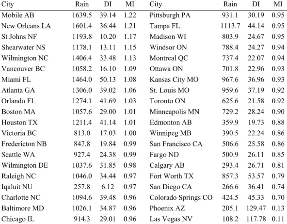
Table 3 gives the moisture indices for the candidate cities used in the MEWS Project. Cornick [24] compares indices for all the candidate cities using both precipitation and aDRI as the wetting index. The approach used in the MEWS project, which was to define the Wetting Index using annual average rainfall, has two advantages:

First, developing wetting indices from annual rainfall is more practical and the data is readily available. It involves considerably less time and fewer resources compared to generating these values from hourly concurrent rain and directional wind data. The moisture index can be reduced to three elements: temperature, humidity, and rainfall.

The MEWS approach can be applied where hourly data are not available.

Second, the normalization scheme can help to set a quantifiable limit on the MI that can be used for Climate Zoning.

(11)

However, like other approaches based on annual rainfall, the MEWS approach to zoning climates does not provide any insight into the severity of wetting on facades, only the relationship between wetting and drying. As with the basic moisture index approach, there is no evidence to support or dispute the weighting of the wetting index to the drying index.

Teq - Equivalent Temperature

The Wetting Index and Drying Index values in all the figures and tables thus far were calculated using hourly data. It is possible to calculate values for the WI and the DI, and consequently the Moisture Index, using single values obtained from climate normal data. For example the WI for a location could be calculated by obtaining the total average annual rainfall from the climate normal data, if rainfall was used as the wetting function. Similarly the DI can be calculated using climate normal data using Equation 10. DI = ∆w(T) = wsat(T) - wout(T) (10)

Where: ∆w is as defined in Equation 4 and T is the annual average temperature from the climate normals (

°

C)

Note that annual average RH is required to calculate wout.

This approach may be useful in regions with sparse networks of hourly reporting stations. MI is intended to be part of an integrated approach to moisture management, and as such it will have to be made available for many locations.

Using long-term climate data the calculation for the MI becomes relatively simple and reduces the effort in calculating the MI for a large number of locations.

Using climate normals to calculate the Drying Index, however, can lead to significant errors in the value of the DI. The annual average temperature T generally underestimates the value of the DI. The reason is that vapour pressure increases nonlinearly as the temperature rises; hence the humidity ratio and temperature are not linearly related.

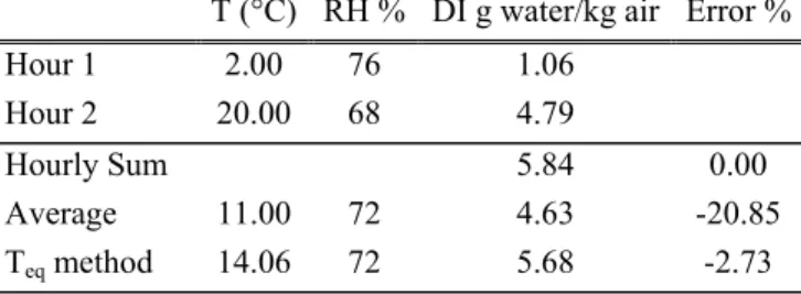
Three methods for calculating the DI were compared: (1) the hourly method, considered to be exact, (2) the average annual temperature (annual) method, and (3) the equivalent temperature method, to be discussed below. The value of the DI is given for each method. Averaging the temperature and relative humidity underestimates the DI by 21%. Averaging the hourly data does not give sufficient credit to the potential evaporation occurring during hours with higher temperatures. This point is illustrated in Table 4 where three different methods for calculating the Drying Index are given for two hypothetical hours. The results of calculating DI using the hourly method, an average temperature approach, and the equivalent

temperature method are shown in Figure 9.

The equivalent temperature T*eq is defined as the equivalent average annual temperature which theoretically

gives the same value for the DI as the hourly method. The relative humidity at T*eq is assumed to the value

obtained from the climate normals, the annual average. By back-calculating for the temperature using the equations for the drying index an exact value of T*eq can be obtained. T*correct is the correction temperature

applied to the average annual temperature, T, obtained from the climate normals, to obtain T*eq. T*correct is

simply the difference between the equivalent temperature and the average annual temperature.

An estimate of T*correct can be calculated from the annual range. The annual range (AR) is defined as the

difference between the maximum of the monthly average temperatures and the minimum of the average monthly temperatures. T*correct is linearly related to the AR. An estimate of the equivalent temperature, Teq

is simply the sum of the annual average temperature, T, obtained form climate normals and an estimate of Tcorrect. This methodology was adapted from Bailey [22].

Tcorrect = 0.2206 * AR - 0.9073 (11)

(12)

Teq = T + Tcorrect (12)

Where:

T is the annual average temperature form the climate normals (

°

C) Tcorrect is the correction factor specified above (°C)

The improvement in the estimate of the Drying Index by using equivalent temperature when calculating the DI from climate normal data is shown in Figure 10. See MEWS [24] for a complete description of the equivalent temperature method.

Climate Zoning

Grouping Climates

Having established the Moisture Index as a procedure for ranking climates, the next step was to establish a method of grouping like climates with respect to potential moisture related problems. Each grouping can be shown as a zone on a map of North America. Since the MI for a location is defined as the distance that the location's climate lies from the origin on a normalized plot (see Figure 11) the boundary values for the groupings can be expressed as radii.

Suppose a particular location has a normalized wetting index, WInormalized, of one, indicated maximum

wetting potential, and a normalized drying index, DInormalized, of one, indicating maximum drying potential.

This climate corresponds to the point (1, 0) on the plot shown in Figure 11. Note that 1 - DInormalized rather

the DInormalized is plotted on the y-axis. This ranking corresponds to a radius, r, equal to one. Similarly a

climate having WInormalized = 0, minimum wetting, and DInormalized = 0, minimum drying, corresponds to the

point (0, 1) in Figure 11. This climate also lies on the arc r = 1.

Although both these climates might differ in terms of wetting (rainfall) and drying (difference in humidity ratios) characteristics the hypothesis is that they are in similar with respect to the potential for moisture related problems. Using an analogy to Mohr's circle the points along a radius are hypothesized to have an equal potential for moisture related problem; an isopotential.

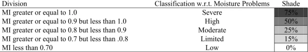
A simple classification can be constructed by splitting the range of the moisture index into a number of divisions. Each division represents a limit for moisture related problems. Climates are then grouped accordingly.

Illustration of the Technique: A Provisional Map

An important output of the MEWS project is the provisional climate map produced using the moisture index approach. A detailed map of the USA and Canada was constructed using 383 stations reporting hourly data. The rankings for each station were calculated using long-term data obtained from climate normals. The current climate normals span the years 1961 to 1990. The Wetting Index was defined, as before, as the annual average rainfall. The Drying Index was computed using the method described except that the average annual temperature and average annual relative humidity was used instead of hourly values. The equivalent temperature method was used to calculate the DI.

One further change was introduced in producing the provisional climate map. The maximum rainfall used to normalize the Wetting Index was set at 2000 mm. Suppose we exclude the exposed Pacific Northwest sites, i.e. those with rainfall > 2000 mm from our proposed zoning scheme for the rest of North America (see Figure 12 and Table 5). Such regions are extreme and not typical of the North American climate. This is not to say that this excluded region will not be subject to moisture problems. In fact all locations that report rainfall in excess of 2000 mm are classified as severe in our scheme. Our reason for removing this

(13)

region from consideration is that its inclusion with the rest of North America tends to skew the rankings, placing regions with an identified history of problems into zones with regions that do not have problems. There is a loss of resolution in the range of interest. We can do a better job of ranking if we break the geographical area into two parts to be handled separately. Or to put it another way, this is like fitting two parts of a complicated set of data with two different curves. That way, two simpler, lower-order curves can give a better fit than one higher-order curve for both parts taken together. The Drying Index was left unchanged since the range of the initial 40 candidate cities adequately covered the range of drying potentials for Canada and the United States.

Five divisions appear on the provisional map shown in Figure 13. The classifications are severe, high, moderate, limited, and, low. A classification of extreme is given to all stations having a ranking of greater than 1.414. The thresholds used in the classification are given in Table 6. In creating the provisional map all extreme stations were included in the severe category. The map shows good agreement with other construction-related climate classification schemes such as Lstiburek [17] and Russo [18].

A few comments on the provisional contour map are worth mentioning.

• First, in generating a contour map a certain amount of information is lost.

• Second, the network of reporting stations used to generate the map is sparse in the northern regions of the continent.

• Third, the selection of the MI defining limits to various climates regions is not related to experimentally observed data.

Conclusions

For the purposes of characterizing climates for moisture related problems in building envelopes, climate can be described using two indices, a Wetting Index which is a function of rainfall, and a Drying Index which is function of potential evaporation. These two indices are independent. Climates can be classified by defining a Moisture Index that combines the Wetting and Drying Indices. The MI can then be used to rank weather stations in a climate classification scheme. Thus climates with dissimilar wetting and drying characteristics can be compared directly using the MI. The moisture index can be considered as an indicatorof potential moisture related problems in building envelopes. Isopotential lines can be created by joining stations with similar moisture indices. Maps showing the potential for moisture related problems could be drawn. Selecting the values of the isopotentials completes the classification scheme. The context of the term ‘moisture related problems in building envelope’ however is general. Different climate classifications can be developed to be used for example at the special problems of wooden buildings and different at the moisture deterioration assessment of the surface layers, or for the selection of Moisture Reference Years for hygrothermal simulations. Future applications should define the field for the potential use of the suggested Moisture Index and then verify the applicability of the index in the chosen field. Several issues remain to be resolved in relation to the Moisture Index approaches to climate classification for construction. Four main issues are:

1. Relative comparisons - The ranking of climates and reference moisture years is based on a relative ranking rather than objective criteria. The lack of objective criteria and hence the relative ranking scheme is a direct consequence of not specifying what constitutes a moisture problem.

Consequently the analysis of climate did not include the wall response to environmental conditions.

2. Equal weighting of the WI and the DI - The assumption is that the wetting and drying indices have equal weights when combined. This may or may not be correct. Again this is due to the initial decision not to consider the wall response.

3. Selecting values of the isopotentials for climate zoning - The authors made arbitrary choices to illustrate the method, specifically the threshold limits used to make the provisional map. To obtain

(14)

meaningful values, decisions must be made as to what factors relate to long-term wall

performance. Here are some examples: decay, corrosion, staining, finish deterioration, production of molds and spores, loss of structural capacity, degradation of thermal resistance, water damage to interior finishes and furnishings, and dimensional changes affecting the appearance or functioning of the wall system.

4. The wind and the wind direction (as well as solar effects) are excluded. The wind and wind direction exclusion can cause a significant increase of the Wetting Index value in case of some continental cities A version of the Moisture Index based on driving rain from the predominant direction for each locality may prove to be a more useful scheme. This would entail a

considerable, although not impossible, amount of work, however, since coincident wind, rain, and solar data are not as ubiquitous as temperature and rainfall.

There are issues that warrant further investigation with respect to the general Moisture Index approach. The two main issues are:

1. No recognition of spells or dry periods - The work presented here is based on an annual analysis. Looking at climate from the perspective of wetting spells and drying periodswas not presented here.

2. Seasonal effects not considered - This is similar to the criticism of not recognizing wet spells. Wetting is strongly dependent on the rain regime of the climate under consideration, the winter rain regime of subtropical dry summer (Cs) climates for example. Should credit be given to the drying potential in the summer when little or no rain falls? Similarly should credit be given to the drying potential during the low sun period in cold climates (Dcb) where most of the precipitation falls as snow?

In summary, determining the potential for moisture related problems for various climates, as well as individual years, can be done using a simple method that uses readily available climate data, specifically climate normal data. The methodology is general and flexible and involves defining a Wetting Index, based on the availability of water, and a Drying Index, based on potential evaporation. These indices are

combined to form a Moisture Index. By redefining the WI and or the DI, as well as changing the relative weighting, a number of specific construction-related climate classifications and maps can be produced.

Acknowledgements

The authors would like to thank the following people, all from the Institute for Research Construction, National Research Council of Canada, for their invaluable assistance:

G. Adaire Chown, Reda Djebbar, Kumar Kumaran, Mostafa Nofal, Michael Swinton, Fitsum Tariku, and a special thanks to Nady Said and Michael Lacasse.

Appendix

Calculating Driving-Rain Loads on Walls

Straube's Method [12]

The method recommended by Straube was selected as the method for calculating the wind driven rain loads (WDR) in IRC's Advanced Hygrothermal Model (HygIRC) and was used in MEWS Task 4 for determining the predominate rainfall directions and moisture reference years (MRY). While Straube recommended using D50 for the raindrop diameter, the predominant raindrop diameter, Dpred, was used. The

(15)

height of the wind speed measurements was assumed to be 10 m. The top corner of the building was assumed to be the location of interest. This was used in determining the RAF factor.

WDR = RAF * DRF(rh) * cos(θ) * V(h) * rh (A.1)

Where: WDR is the wind driven load (l/m2-h) RAF is the rain admittance factor

rh is the horizontal rainfall intensity (mm/m2-h)

V(h) is the wind speed at the height of interest (m/sec)

θ is the angle of the wind to the wall normal

The rain admittance factor, RAF, was provided by Straube (assumed to be 0.9). The driving-rain factor can by calculated from:

DRF(rh) = 1/Vt (A.2)

Where: DRF is the driving-rain factor

Vt is the terminal velocity of raindrops (m/sec)

The terminal velocity can be calculated from Dingle and Lee [28]:

Vt(Φ) = -0.16603 + 4.91884 * Φ - 0.888016 * Φ2 + 0.054888 * Φ3 <= 9.20 (A.3)

Where: Vt(Φ) is the terminal velocity of a raindrop of diameter Φ in still air (m/sec)

The distribution of raindrop sizes for a given horizontal rain intensity is given by Best [29]. F(Φ) = 1 - exp{-(Φ/(1.30 * rh0.232))2.25} (A.4)

Where: F(Φ) is the cumulative probability distribution of raindrop sizes for rh (mm)

Φ is the equivalent spherical raindrop diameter (mm)

D50 is the value of the drop diameter x such that 50 percent of the water in the atmosphere is comprised of

drops with a diameter less than D50. The predominant drop diameter, Dpred, is the diameter of drops that

accounts for the greatest volume of water in the air.

D50 = a * 0.691/n (A.5)

Dpred = a * ((n - 1)/n)1/n (A.6)

Where: a = 1.30 rhp, p = 0.232

n = 2.25

References

[1] Trewartha, G. T., An Introduction to Climate 4th Edition, McGraw-Hill, New York, 1968. [2] Hoppestad, S. Slagregn I Norge, Norwegian Building Institute, Oslo, Rapport Nr. 13. 1955. [3] Lacy, R. E., "Driving-Rain Maps and the Onslaught of Rain on Buildings", Proceedings of the RILEM/CIB Symposium on Moisture Problems in Buildings, Helsinki Finland, 1965.

[4] Straube, J.F. and Burnett, E.F.P., (2000), "Simplified prediction of driving rain deposition", Proceedings of International Building Physics Conference, Eindhoven, September 18-21, pp. 375-382.

(16)

[5] Boyd, D. W., Driving Rain Map of Canada, Technical Note 398, Division of Building Research, National Research Council of Canada, Ottawa, 1963.

[6] Underwood, S. J., and Meentemeyer, V., "Climatology of Wind-Driven rain for the Contiguous United States for the Period 1971 to 1995", Physical Geography, 1998, 19,6:445-462.

[7] Cornick, S. M. and Chown, G. A., "Defining Climate Regions as a Basis for Specifying Requirements for Precipitation Protection for Walls, Ottawa: Canadian Commission on Building and Fire Codes, National Research Council of Canada, pp. 36, April 12, 2001 (NRCC-45001)

[8] Choi, E. C. C., "Parameters Affecting the Intensity of Wind-Driven Rain on the Front Face of a

Building", Proceedings of the Invitational Seminar of Wind, Rain, and the Building Envelope, University of Western Ontario, London, Canada, May 16-18, 1994.

[9] Blocken B., and Carmeliet, J., "Driving rain on buildings envelopes - I. Numerical estimation and full scale experimental verification" Journal of Thermal Envelope and Building Sciences, 2000, 24, 1, 61-84. [10] Blocken B., and Carmeliet, J., "Driving rain on buildings envelopes - II. Representative experimental data for driving rain estimation" Journal of Thermal Envelope and Building Sciences, 2000, 24, 2, 89-110. [11] Prior, M. J., Directional driving rain indices for the United Kingdom - computation and mapping: background to BSI Draft for Development DD93, Building Research Establishment Report, Dept. of the Environment, Building Research Establishment, Building Research Station, 1985.

[12] Straube, J. F., Moisture Control and Enclosure Wall Systems, Ph.D. Thesis, Civil Engineering Department, University of Waterloo, 1998.

[13] Choi, E. C. C., "Numerical simulation of wind-driven rain falling onto a 2-D building.", Proceedings of the Asian Pacific Conference on Computational Mechanics. Hong Kong, Hong Kong, Nov 11-13, 1991. pp.1721-1727.

[14] Hagentoft, C. and Högberg, A., "Prediction of driving rain intensities using potential flows", 6th Symposium on Building Physics in the Nordic Countries, Trondheim, Norway, Jun 17, 2002.

[15] BSI. British Standard Code of Practise for Assessing the Exposure of Walls to Wind-driven Rain, BS 8104, British Standards Institution 1992.

[16] CEN prEN ISO 15927-3, Hygrothermal performance of buildings - Climatic data - Part 3: Calculation of a driving rain index for vertical surfaces from hourly wind and rain data. TC 89 Thermal performance of buildings and building components, WG 9 Climatic Data. Under approval, 2003.

[17] Lstiburek, J. W., "Hygrothermal Climate Regions, Interior Climate Classes, and Durability",

Proceedings of the Eighth Conference on Building Science and Technology, Toronto, Canada, February 22-23, 2001. pp. 319-329.

[18] Russo, J. A., The Complete Money-Saving Guide To Weather For Contractors, Environmental Information Services Associates, Connecticut, USA, 1971. pp. 78-79.

[19] Scheffer, T. C., "A Climate Index for Estimating Potential for Decay in Wood Structures above Ground", Forest Product Journal, 1971 21:25-31.

[20] Setliff, E. C., "Wood Decay Hazard in Canada Based on Scheffer's Climate Index Formula", The Forestry Chronicle, October 1986: 456-459.

(17)

[21] Carter, J.O., Cause, M.L., and Moffat, A. "A preliminary above- ground wood decay index map of Australia." Paper presented at 25th Forest Products Research Conference, CSIRO, Clayton, Victoria. 1983 [22] Bailey, H. P., "A Simple Moisture Index Based Upon a Primary law of Evaporation", Geog. Ann., 1958, 40: 196-215.

[23] Mather, J., R., and Yoshioko, G., A., "The Role of Climate in the Distribution of Vegetation." Annals, Assoc. Am. Geogr., 1968, 58: 29-41.

[24] Cornick, S. M., Dalgliesh, W. A., Said, N. M., Djebbar, R., Tariku, F., Kumaran, M. K., Report from Task 4 of MEWS Project - Task 4 Environmental Conditions Final Report, Research Report IRC-RR-113, Institute for Research in Construction, National Research Council of Canada, October 01, 2002.

(http://irc.nrc-cnrc.gc.ca/bes/mews/reports.html)

[25] Hagentoft, C. E., Harderup, E., "Climatic Influences on the Building Envelope Using the Π Factor", IEA-Annex 24 Hamtie Task 2, Environmental Conditions. Closing Seminar, Finland 1996.

[26] Beaulieu, P.; Bomberg, M.; Cornick, S.; Dalgliesh, A.; Desmarais, G.; Djebbar, R.; Kumaran, K.; Lacasse, M.; Lackey, J.; Maref, W.; Mukhopadhyaya, P.; Nofal, M.; Normandin, N.; Nicholls, M.; O'Connor, T.; Quirt, J.; Rousseau, M.; Said, M.; Swinton, M.; Tariku, F.; van Reenen, D.

Final Report from Task 8 of MEWS Project (T8-03) - Hygrothermal Response of Exterior Wall Systems to Climate Loading: Methodology and Interpretation of Results for Stucco, EIFS, Masonry and Siding Clad Wood-Frame Walls, Research Report IRC-RR-118, Institute for Research in Construction, National Research Council of Canada, November 01, 2002. (http://irc.nrc-cnrc.gc.ca/bes/mews/reports.html) [27] Cornick, S.M.; Dalgliesh, W.A. "A Moisture index approach to characterizing climates for moisture management of building envelopes," 9th Conference on Building Science Technology, Vancouver, British Columbia, February 01, 2003, pp. 383-398,

[28] Dingle, A. N., and Lee, Y., "Terminal Fall Speeds of Raindrops", J. of Appl. Meteor., Vol. 11, August 1972, pp. 877-879.

[29] Best, A. C., "The Size Distribution of Raindrops", Quarterly Journal of Royal Meteorological Society, 1950 76:16-36

(18)

Figure Captions

Figure 1. Climate-index map of Canada prepared from the formula given by Scheffer. The three zones represent three levels of above ground wood decay potential, after Setliff [20].

Figure 2. The plots show the monthly climate normal rainfall and average temperature for a) Vancouver BC, b) Ottawa ON. The left axis reports the normal monthly rainfall while the right axis shows the normal monthly average temperature.

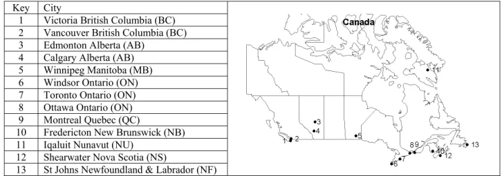
Figure 3. The plot shows the west to east progression of the drying index, DI. Generally both coasts of North America have lower drying potentials than continental locations. The exception is Iqaluit, north of the Arctic Circle. The climate is simply too cold to allow significant amounts of evaporation. The key for the location codes is given in Table 2 along with a small map.

Figure 4. West to east progression of the wetting index, WI as annual rainfall and rain load on the wall in the worst direction.

Figure 5 West to east progression of MI normalized, where MI 1 is based on annual rainfall and MI 4 is based on rain load impinging on a wall with the most severe exposure calculated using Straube's method. A clear distinction is made between the coastal and continental climates.

Figure 6. West to east progression of the MEWS Moisture Index, which is based on annual average rainfall from climate normal data. Except for magnitude the result is similar to the previous approaches.

Figure 7. The plot shows DI and WI for individual years for five selected cities. The plot shows the range and variability of both indices as well as the relative characterization of the general climates found in those cities.

Figure 8. A plot of 1 - normalized Drying Index versus normalized Wetting Index (precipitation) for the candidate cities. The moisture index is calculated as the distance from the origin.

(19)

Figure 9. The chart shows the error introduced into the drying index by averaging temperature and relative humidity data. The error in this case is -21%. Using the equivalent temperature method the error is reduced to about -3%.

Figure 10. The plot shows a comparison between the annual and equivalent temperature methods for calculating the drying index. The 40 candidate cites are shown. The equivalent temperature method performs better the annual method when compared to the values calculated using the hourly method, assumed to be exact.

Figure 11. The plot shows a classification scheme based on a hypothesis of isopotentials. Each radius defines a locus of points having an equal potential for moisture related problems.

Figure 12. The map shows the location of all the continental stations considered that report more than 2000 mm of rainfall. They are all on the North American northwest coast littoral. These stations are considered extreme with respect to moisture related problems.

Figure 13. The contour map shows the isopotential lines for moisture related problems. The classification is based on five divisions of the range of values of the moisture index. 383 hourly reporting stations were used to generate the map. The reporting stations are shown as points on the map.

(20)

Table s

Russo's criteria

Zone Description Jan. Min. Avg. Temperature Annual Avg. Rainfall Zone 1 Cold and Wet Less then 15 oF More than or equal to 20

inches

Zone 2 Cold and Dry Less then 15 oF Less than 20 inches Zone 3 Mild and Wet 15 oF to 30 oF More than or equal to 20

inches

Zone 4 Mild and Dry 15 oF to 30 oF Less than 20 inches Zone 5 Hot and Wet More than 30 oF More than or equal to 20

inches

Zone 6 Hot and Dry More than 30 oF Less than 20 inches ● note that 15 o

F ~ -9.5 oC; 30 oF ~ -1 oC; 20" ~ 500 mm Table 1. Russo's construction related climate classification.

(21)

Key City

1 Victoria British Columbia (BC) 2 Vancouver British Columbia (BC) 3 Edmonton Alberta (AB) 4 Calgary Alberta (AB)

5 Winnipeg Manitoba (MB) 6 Windsor Ontario (ON) 7 Toronto Ontario (ON) 8 Ottawa Ontario (ON) 9 Montreal Quebec (QC) 10 Fredericton New Brunswick (NB) 11 Iqaluit Nunavut (NU)

12 Shearwater Nova Scotia (NS)

13 St Johns Newfoundland & Labrador (NF)

(22)

City Rain DI MI City Rain DI MI Mobile AB 1639.5 39.14 1.22 Pittsburgh PA 931.1 30.19 0.95

New Orleans LA 1601.4 36.44 1.21 Tampa FL 1113.7 44.14 0.95 St Johns NF 1193.8 10.20 1.17 Madison WI 803.9 24.67 0.95 Shearwater NS 1178.1 13.11 1.15 Windsor ON 788.4 24.27 0.94 Wilmington NC 1406.4 33.48 1.13 Montreal QC 737.4 22.07 0.94 Vancouver BC 1058.2 16.10 1.09 Ottawa ON 701.8 22.96 0.93 Miami FL 1464.0 50.13 1.08 Kansas City MO 967.6 36.96 0.93 Atlanta GA 1306.0 39.02 1.06 St. Louis MO 959.6 37.19 0.92 Orlando FL 1274.1 41.69 1.03 Toronto ON 625.6 21.58 0.92 Boston MA 1057.6 29.00 1.01 Minneapolis MN 729.2 28.24 0.90 Houston TX 1211.4 41.14 1.01 Edmonton AB 359.9 19.73 0.88 Victoria BC 813.0 17.03 1.00 Winnipeg MB 390.5 22.24 0.86 Fredericton NB 847.8 19.84 0.99 San Francisco CA 506.6 25.58 0.86 Seattle WA 927.4 24.38 0.99 Fargo ND 500.9 26.11 0.85 Wilmington DE 1037.6 31.85 0.98 Calgary AB 293.4 26.71 0.81 Raleigh NC 1046.0 34.44 0.97 Fort Worth TX 857.3 53.57 0.79 Iqaluit NU 257.8 6.12 0.97 San Diego CA 266.6 36.41 0.74 Charlotte NC 1094.6 39.48 0.96 Colorado Springs CO 424.5 45.33 0.70 Baltimore MD 1026.1 34.87 0.96 Phoenix AZ 205.1 129.47 0.13 Chicago IL 914.3 29.01 0.96 Las Vegas NV 108.2 117.78 0.11 MI is based on hourly values; Rainfall is in mm; DI is kg water/kg air. To calculate MI use the procedure outlined above. Normalize the wetting index using Mobile AB. Normalize the drying index using Phoenix AZ.

(23)

T (°C) RH % DI g water/kg air Error % Hour 1 2.00 76 1.06 Hour 2 20.00 68 4.79 Hourly Sum 5.84 0.00 Average 11.00 72 4.63 -20.85 Teq method 14.06 72 5.68 -2.73

(24)

WBAN Station Name State Rainfall (mm) T (C) RH % 25339 YAKUTAT AK 3349.0 3.9 80.5 94234 TOFINO A BC 3235.8 9.0 85 94240 QUILLAYUTE WA 2638.3 9.4 83 25308 ANNETTE AK 2501.1 7.7 76.5 25353 PRINCE RUPERT A BC 2409.1 6.9 82 * Note the low temperatures and high RH and Rainfall on the Northwest coast of NA

(25)

Division Classification w.r.t. Moisture Problems Shade

MI greater or equal to 1.0 Severe 75%

MI greater or equal to 0.9 but less than 1.0 High 50% MI greater or equal to 0.8 but less than 0.9 Moderate 25% MI greater or equal to 0.7 but less than .0.8 Limited 15%

MI less than 0.70 Low 0%

Table 6. Thresholds used to delimit climate zones used in making the provisional map.

(26)

(27)

Decay Hazard

(Scheffer's Index)

High > 70

Moderate 35 - 70

Low < 35

Figure 1

(28)

0

5

10

15

20

25

30

35

40

45 Jan

Feb

_Mar

Apr

_May

Jun

Jul

_Aug

Sep

Oct

_Nov

Dec

(a)

Average Monthly Temperature (C)

-15

-10

-5

0

5

10

15

20

25

30 Rainfall (cm)

Ann. rainfall (mm)

Ann. avg temp (C)

Temperate Oceanic Cool Summer (Dob)

Vancouver, Canada

1167.4

9.9

(29)

0

5

10

15

20

25

30

35

40

45 Jan

Feb

_Mar

Apr

_May

Jun

Jul

_Aug

Sep

Oct

_Nov

Dec

(b)

Average Monthly Temperature (C)

-15

-10

-5

0

5

10

15

20

25

30 Rainfall (cm)

Ann. rainfall

Ann. avg temp (C)

Temperate Continental Cool Summer (Dcb)

Ottawa, Canada

700.5

6

(30)

NOTE that it would be ideal to place the images side by side to allow for direct comparison. See the sample layout above. Note that the above image is not the one intended for publication.

(31)

West to East Progression of the Drying Index

0

5

10

15

20

25

30

1

2

3

4

5

6

7

8

9

10

11

12

13 Location

Drying Index (kg water/kg air/year)

(32)

West to East Progression of the Wetting Index

0

200

400

600

800 1000

1200

1400

1

2

3

4

5

6

7

8

9

10

11

12

13 Location

Wetting Index (l/m2/year)

0

0.1

0.2

0.3

0.4

0.5

0.6

0.7

0.8

0.9

1

Annual Rainfall Straube's Method normalized Straube normalized Rain Figure 4