Active torque ripple reduction in permanent-magnet AC motors

Active Torque Ripple Reduction in Permanent-Magnet AC Motors

Christopher Anthony Greamo

B.S., Electrical Engineering Carnegie-Mellon University, 1993

Submitted to the Department of

Electrical Engineering and Computer Science in Partial Fulfillment of the Requirements for the

Degree of

MASTER OF SCIENCE in Electrical Engineering

at the

Massachusetts Institute of Technology

June 1995

© 1995 Christopher A. Greamo All Rights Reserved

The author hereby grants to MIT permission to reproduce and to distribute publicly paper and electronic copies of this thesis

document in whole or in part.

Signature of Author

-Department of EECS April 13, 1995

Certified by -

-

-Bernard C. Lesieutre Ax arkb Assist. Professor, EECS Department

n".

.

Thesis

Supervisor

Accepted by

-1

\ \ Frederic R. Morgenthaler

Chairman' ommittee on Graduate Students

Acknowledgments

I would like to offer my sincere thanks to a number people without

whom completion of this project would not have been possible. To my

advisor Dr. Bernard("Bernie") Lesieutre not only for his technical knowledge

and insights, but also for his enthusiastic support of the project. To Scott

Ellerthorpe, Peter Cho, Andrew Bedingfield of the Naval Undersea Warfare Center(NUWC) in Newport, R.I. and Dr. Duane Hanselman of the University of Maine for their individual insights into the physics of electric motors. To Andrew Barnett, John Raposa, and Dan Thivierge also of the NUWC for their combined technical assistance in the laboratory.

I would also like to offer thanks to my family and friends, especially to

my girlfriend, Annukka, and my parents, Juliann and Anthony for their

Active Torque Ripple Reduction in Permanent-Magnet AC Motors

by

Christopher Anthony Greamo

Submitted to the Department of Electrical Engineering and Computer Science on April 13, 1995 in partial fulfillment of the requirements for the Degree of Master of Science in

Electrical Engineering

Abstract

Autonomous Underwater Vehicles (AUVs) pose a unique challenge in the design of motor drive systems. The motor is required to be low weight

and to produce high torque with high efficiency and reliability.

Permanent-magnet AC (brushless DC) motors are well suited for this application.

However, it is highly desirable that the motor work quietly to avoid

disturbing the environment and/or detection. Unfortunately,

permanent-magnet motors tend to have high torque ripple in trade-off for their high

output torque and efficiency which results in persistent noise transmission

with a well defined signature. The focus of this thesis is the study of torque

ripple reduction methods for permanent-magnet motors in an attempt to

design a drive system with high power density coupled with low torque

ripple.

In this study, active shaping of the stator current waveforms is used to cancel torque ripple due to both slot harmonics and cogging effects. Both

problems of current waveform selection and enforcement are addressed. A

unique close-loop approach to selecting the appropriate current harmonics

using estimates of the torque ripple spectrum from a load torque

measurements is discussed. The scheme uses a model reference adaptive control algorithm which requires no a priori knowledge of motor parameters.

A pulse-width modulation(PWM) scheme for imposing the current

waveform on the stator windings with minimal phase and amplitude

distortion is also presented. Detailed simulation results are provided which

indicate that a better 80 dB reduction in torque ripple through active current

control is possible without a significant reduction in the system's power

efficiency.

Thesis Supervisor: Dr. Bernard L. Lesieutre

Table of Contents

1.

Background

Page 6

1.1 Autonomous Underwater Vehicles (AUVs) ... 6

1.2 Permanent-Magnetic AC Motors . . ... 6

1.3 A xial-Field M otors ... 7

1.4 Existing Torque Ripple Reduction Methods ...9

2. System Modeling Page 11 2.1 The Three-Phase Permanent-Magnet AC Motor (PMAC) ... 11

2.2 Tangential Torque in PMAC Motors ...16

2.3 Axial Forces in Axial-Field PMAC Motors ...21

3.

Active Torque Ripple Reduction

Part I: Current Selection

Page 23

3.1 Harmonic System Analysis ... 23

3.2 Harmonic Analysis of PMAC Motor ...28

3.3 Minimum Torque Ripple Controller ...35

3.4 Harmonic System Simulation & Parameter Estimation ...39

4.

Active Torque Ripple Reduction

Part II: Current Enforcement

Page 51 4.1 The Current Controlled Voltage Source Inverter (CCVSI) ...51

4.2 Standard Pulse-Width Modulation(PWM) Schemes ...55

4.3 Model Reference PWM Scheme ... 57

4.4 Model Reference PWM CCVSI Simulation ... 60

4.5 Model Reference PWM CCVSI Experimental Results ...67

5.

Practical Issues

Page 74 5.1 Power Electronic Limitations . ... ... 74

6.

Detailed System Simulation

Page 78

6.1 Simulation Parameters ... 78

6.2 Simulation Results ... 79

6.2.1 Baseline Simulation ... 79

6.2.2 Active Torque Ripple Reduction Simulation ...86

6.2.3 Limited Current Harmonics Cases ...91

6.2.4 Extended Simulation Run ... 94

7. Conclusions Page 99 7.1 Contributions ... 99

7.2 Summary of Results ... 100

7.3 Future Work ... 1...100

1 Background

1.1 Autonomous Underwater Vehicles (AUVs)

Autonomous

Underwater Vehicles or AUVs are unmanned,

submarine type vehicles which are designed to infiltrate and investigate

dangerous or otherwise inaccessible underwater environments. Figure 1.1 is a non-scale depiction of an AUV.

Figure 1.1: Side-View Sketch of AUV

The vehicles are completely self-contained. They usually use an electric drive system powered by internally carried batteries, and follow a pre-programmed mission with little or no external guidance. For this reason, power efficiency and system reliability are key design constraints.

The heart of many AUV missions is the collection of intelligence with

minimal disturbance to the environment under observation. For military

scenarios, stealth is especially important for mission success and vehicle survivability. To this end, it is important for the AUV drive system to operate

relatively noise-free while maintaining high efficiency and reliability. A

major noise source in electric motor drives is torque ripple or a variation in

the motor's torque production due to unavoidable imperfections in the

motor's construction. This torque ripple can excite mechanical modes in the

drive shaft which transmit sounds at discrete frequencies into the

environment defining an easily recognizable signature for the vehicle. The effect is most pronounced during low speed operation. For this reason, much effort has been directed by the U.S. Navy into understanding the causes torque ripple and developing methods to reduce it.

1.2 Permanent-Magnet AC Motors

Recent technological developments have made Permanent-Magnet AC or PMAC motors a viable choice for an AUV drive system. High power density permanent-magnet material can be used to make light-weight motors

capable of delivering very high torque[7]. Advances in power electronic

devices and circuits result in highly efficient and reliable drive systems.

Figure 1.2: Cross Section of a Three-Phase Radial-Field PMAC Motor

An important engineering trade-off in PMAC motor design is power density and torque ripple[6]. In many PMAC motors, neither the stator nor the rotor have smooth profiles(Figure 1.2). Slots on the stator for the phase windings and the permanent magnet pieces on the rotor cause a "jagged" interface between the stator and rotor edges. Due to this saliency, the total tangential force on the rotor is not constant over all rotor positions. The forces caused by the interaction between a rough stator and the rotor are called "cogging" and "reluctance" torques. In a rotating machine, such as an AUV drive system, these torques produce periodic vibrations in the motor's total output torque and is one source of torque ripple.

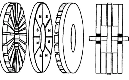
1.3 Axial-Field Motors

Radial-Field PMAC motors, like the one depicted in Figure 1.2, are not the only PMAC configuration. Instead of surrounding the permanent-magnet

rotor radially by the stator, the rotor and stator may be stacked axially as

shown by Figure 1.3. The magnetic flux lines pass through the rotor parallel to the drive shaft(i.e. along the axial direction) instead of radially outward from the center of rotation. Note that the direction of the resulting force on the rotor is tangential(i.e. the same) for both configurations.

Figure 1.3: Side View of A Dual-Stator Axial-Field PMAC Motor

One major benefit of the axial-field configuration is the ability to use two stators, one placed on either side of the rotor. This feature allows high torques and efficiency, which are desirable for AUV drive systems.

stator

Figure 1.4: Aligned vs. Misaligned Rotor

There are two main drawbacks to the axial-field motor. One is the

complexity of construction. Not only are there more basic pieces to the motor, alignment of the rotor between the two stators becomes a key issue(Figure 1.4). It has been shown in reference[6] that the motor performance is sensitive to even a small rotor misalignment. Secondly, axial-field motors suffer from

larger torque ripple than equally sized radial-field motors. This torque ripple

can have both an axial and tangential component in axial-field motors

whereas traditional radial-field motors only have a tangential component.

ripple reducing techniques to realize the benefits of an axial-field

configuration.

1.4 Existing Torque Ripple Reduction Methods

Torque ripple is considered a parasitic component in most motor

systems. Electric machines are constructed in such a way to minimize the

torque ripple component for the intended operational speed. This is done

through the skewing of slots along the stator or other geometric variations in

the motors construction(references [6], [9], and [14]). In vehicle drive

applications, however, the requirements for high power and high efficiency

make torque ripple minimization through motor design difficult. Drive

systems are often required to operate over a wide speed range, making torque

ripple minimization for the entire operational range nearly impossible

through a fixed geometry design.

Research into torque ripple reduction through the shaping of the phase current waveforms has shown promise. Reference[2] includes an analysis of

the physics of torque ripple in brushless DC motors and shows that the

"optimal" phase current waveforms for ripple-free operation can be

computed, in theory, given the motor's back electro-motive force (EMF)

shapes. This work is extended in reference[3] in which an open-loop current controller was proposed and shown through computer simulation to produce

ripple-free operation. Although this work provided insight into the origins

of torque ripple in machines and provided motivation to the possibility of using control of phase currents to reduce torque ripple, the open-loop scheme

did not address the issues of system stability, transient response, and

robustness to parameter variations and assumes precise a priori knowledge of

the motor's parameters.

A controls oriented approach to the problem of torque ripple

cancellation is pursued in references [4] and [5] where an adaptive feedback

controller is proposed that cancels torque ripple harmonics through the

controlled addition of harmonics to the phase current waveform. Position

and velocity feedback are used to "adapt" the magnitude of the applied

current harmonics in real-time. System stability and robustness can be

proven, and the controller requires nearly no knowledge of the motor's

parameters. There are some draw-backs to the approach. It is assumed that the current commands generated by the controller can be exactly followed by the power electronics; there are no limits on the amplitude or rate of change of the commanded phase currents. In addition, there is no clear relationship between applied current harmonics and the physical parameters of the motor. As such, it is not clear the current waveforms generated by the controller are

"optimal" in the same sense shown by reference[3].

Most of the literature on torque ripple reduction has focused on field machines. This is no doubtfully due to the large popularity of the radial-field topology. References [6] and [7] provide a detailed analysis of the sources

of torque ripple in dual-stator axial-field motors and suggest some

construction techniques to reduce the ripple. Little or no research, however, has been published on active torque ripple reduction techniques in axial-field motors. It is the goal of this thesis document to apply some of the existing

knowledge and techniques concerning active torque ripple reduction to this

promising yet under-utilized motor configuration.

2 System Modeling

Proper modeling of the dynamics of the permanent-magnetic motor is key to understanding the source of torque ripple. The following analysis will begin with the generic three phase electric machine equations which can be found in reference [27] and will develop a specific model for a dual-stator,

permanent-magnet motor including tangential torque ripple. Some sources

of axial torque ripple will also be discussed.

Following the model

development, specific conditions for torque ripple free operation will be

derived.

2.1 The Three-Phase Permanent-Magnet AC Motor (PMAC)

A fifth-order dynamic model is used to model the three-phase

permanent-magnet motor used in this study. There are two natural choices for the three electrical state-variables-- either the stator fluxes, Xa, ?b, and Xc, or the stator currents, ia, ib, and ic. Since current control power electronics will be used to drive the stator windings, the phase currents will be chosen as the state-variables. The two mechanical states are co and 0 representing the rotational velocity and position of the shaft, respectfully. By choosing the states in this manner, the motor may be viewed as two coupled subsystems--one electrical, and the other mechanical. This is illustrated in Figure 2.1. Assuming an ideal flux/current relation and constant speed operation, the two subsystems are linear. This property has been exploited by a number of motor speed control schemes[4], [5], [21], and [26].

TI Va Vb Vc e (O

Figure 2.1: Motor System Block Diagram

The inputs Va, Vb, and Vc are the phase winding voltages applied to the electrical subsystem via the stator. The outputs are the mechanical

state-variables 0 and co. Other state-variables of interest include the tangential

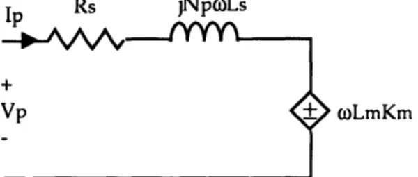
The electrical parameters of the motor include the phase winding

resistance Rs and self-inductance Ls for each of three stator phases, and the mutual inductance Lm linking each of the phases to the magnetic rotor and to each other. The rate of change these inductance terms produces a voltage

known as the excitation voltage whose amplitude is proportional to the shaft velocity . Figure 2.2 is a linear circuit model for the electrical dynamics of a single motor phase.

In Rs jNpoLs

coLmKm

Figure 2.2: Phase Winding Model

For a symmetric three-phase machine, each winding may be modeled

equivalently[38].

One may model the permanent-magnet rotor as another phase

winding carrying constant current[27]. This increases the number of states in the system by one, however this artificial state can be discarded after using it to compute the form of the electrical torque equation, reducing the final model to a fifth-order model.

The vectors corresponding to the flux-linkages, applied voltages, and generated currents are given by Equations (2.1), (2.2), and (2.3).

A= Xc (2.1) V V = (2.2) i=[ ] (2.3)

The top three elements of each vector are the state and input variables for the

three stator phases, labeled a, b, and c. The bottom entries represent the

variables associated with the rotor phase. As is done in reference[27], the

current. This implies an applied voltage of zero(i.e. the bottom entry in

Equation (2.2)) and a constant current(i.e. Km in Equation (2.3) ).

The resistance matrix is given by Equation (2.4) assuming the machine has similar phase windings, each with equal phase resistance Rs.

Rs 0 0 0

R = Rs (2.4)

0 0 Rs

The fourth row and column of R correspond to the artificial rotor winding. Since this winding has a constant current and no applied voltage, it's phase resistant is zero. Equation (2.5) shows the form of the machine's inductance

matrix.

Laa(0) Lab () Lac () Lam()

1

L( Lab(0) Lbb(0) Lbc(0) Lbm(0) (2.5) Lac (0) Lbc(0) Lcc(0) Lc ()

Lam (0) Lbm(0) Lcm(0) Lmm ()

The notation Lxx refers to the self-inductance for phase x, and Lxy is the mutual-inductance between phase x and phase y, where a, b, and c are the

three stator phases and m is the rotor phase. Assuming a symmetric

machine, the stator self-inductances are equal(i.e. Laa=Lbb=Lcc) and all

mutual inductance terms are symmetric(i.e. Lxy=Lyx for all x,y = a,b,c,m). In

this model, all inductance terms are a function of rotor position 0. This

implies that for a rotating motor, L(0) is periodic in 0 with period 2/[ electrical radians(i.e. L(0+2X)=L() ).

There are three fundamental physical equations underlying the

motor's dynamics. Faraday's and Ohm's Laws specify the electrical dynamics,

= V - Ri (2.6)

Newton's Second Law of Motion specifies the mechanical dynamics, [J is the

moment of inertia of the rotor, shaft, and load; Tt is the tangential

component of the electrically generated torque; and TL is the load torque].

dco

Jdo = Tt - TL (2.7)

dt

The second mechanical state, position, is the integral of speed.

dO

dt= o(2.8)

dt

As shown in Equation (2.7), the net torque applied to the rotor at any

given time is the difference between the torque due to the electrical

interactions between the stator windings and the magnetic rotor, and the

mechanical load torque opposing the movement of the shaft. The tangential component of the electrically generated torque Tt is given by Equation (2.9)

[27].

Tt = iT di (2.9)

t2

dO

In an axial-field motor, there are two components to the electrical

torque--tangential and axial. Only the torque--tangential component Tt contributes to

working torque, and therefore, is the only component in Equation (2.7). The axial component Ta contributes only to vibrations of the shaft through excitations of its axial modes. This will be discussed in greater detail in Sections 2.2 and 2.3. The load torque TL is due to frictional forces which

oppose the motion of the shaft in the environment.

Since TL is a

manifestation of frictional type forces, it is some function of the rotor's rotational speed co. For many typical loads, such as a propulsor in a viscous fluid, the load torque is best modeled by a quadratic function.

TL = sgn(co)(Kbco + Kpc02 ) (2.10)

The sgn(co) multiplier insures that the torque always opposes the motion of the shaft.

Since the currents i were chosen as the electrical states, it is necessary to eliminate A, from Equation (2.6) before assembling the equations of the motor into the standard state-space form. Assuming an ideal flux/current relation, the flux vector x can be expressed as the product of the inductance matrix L and the current vector i.

A = Li (2.11)

Taking the time derivative of Equation (2.11) yields Equation (2.12). dA d(Li)

dt

dt

di dL.

= L-+-i

dt

dt

(2.12)

=di dL di

dt dO dt

di

dL

= L +co i dt dO

Finally, substituting Equation (2.12) into Equation (2.6) and collecting like terms yields Equation (2.13).

di dL

L = V - [R + co ]i (2.13)

dt dO

The inductance matrix L must be symmetric and positive-definite for any physically realizable machine(see reference[27] for proof). Thus, L must be invertible(i.e. L-1 )exists. Multiplying Equation (2.13) by L-1 _{yields Equation}

(2.14).

-=

UL

V -- l[R+ e*)-li

(2.14)

dt dO

dtO [ ][ T (i, 0) J TL(W)] (2.15) Together, Equations (2.14) and (2.15) form the state-space model for the

2.2 Tangential Torque in PMAC Motors

As mentioned previously, only the tangential component of torque

contributes to the desired rotational acceleration of the drive shaft, and thus, produces useful work. In radial-field motors, the torque of electrical origin has only a tangential component. In axial-field motors, the generated torque can have both tangential and axial components; the axial component will be further discussed in Section 2.3.

Figure 2.3: Tangential and Axial Torque Components

Equation (2.9) is the general equation for the tangential component of

the torque of electrical origin. This equation is derived from energy

conservation arguments. A detailed formulation can be found in

reference[27]. Expanding the vector symbols in Equation (2.9) with the full matrix and vector representations yields Equation (2.16).

Tt = [ia ib ic km]

dLaa dLab dac dLam

dO dO dO dO dLab dLbb dLbc dLbm dO dO dO dO dLac dLbc dLcc dLcm dO dO dO dO dLam dLbm dLcm dLmm dO dO dO dO ia ib (2.16) kc km

Performing the appropriate matrix multiplication and grouping common

terms gives the scalar Equation (2.17).

T,

(

dLaa 2dLbb dLa dL 2dL dLab i

dL

dLC

a dLb

Tt 2 dOa +ibd +C dO)+(iaib dO aicdO' +lbic dOc

+ k (i dLam + ib dLbm +i dm) (2.17)

dO dO d

+ k2 dLmm m dO

In general, every inductance term will be a function of rotor position 0 and can contribute to the net generated torque. For a rotating machine, these functions will all be periodic with period 2 electrical radians, and therefore, can all contribute to torque ripple. Depending on the motor's construction some terms may be negligible in comparison to others.

The tangential electrical torque Tt has three distinct physical origins. Equation (2.17) can be divided into three component, each representing a different source.

Tt = Tr + Tk + Tc (2.18)

The first component Tr is called reluctance torque.

T.= 1 (.2dLbb i2 + dL) dLacaa dLbc )(2.19) r 2 a dO _do ib + i a aO i i cc+ -- b

b dO c dO dO ac dO dO

As shown in Equation (2.19), the reluctance torque expression contains

products of the electrical state variables (i.e. the stator currents), and thus, is highly nonlinear. This torque component is caused by changes in the stator self-inductances with rotor position. These changes are induced by a time-varying reluctance path for the stator flux caused by rotor saliency. For switched reluctance motors, this component can be large and is the prime

source of working torque. For synchronous PMAC motors, however, the

reluctance torque is usually minimized though the use of a smooth rotor

construction. This is the case for the dual axial-field motor under study here, and therefore, Tr is assumed to be negligible.

The second component T is known as mutual torque, and for PM motors, is the main source of working torque.

T km (ia ib d +iC ) (2.20)

dO dO dO

This component is a function of the mutual inductance between each stator phase and the rotor, and is a linear function of the stator currents. In an ideal

motor, the stator windings would be wound in an exact sinusoidal pattern

Lam = Lm cos(Np0)

Lbm = Lm cos(Npe- ) (2.22)

Lcm = Lm cos(NpO - ) (2.23)

Note that the period of the inductance functions are dependent on the

number of pole pairs Np. Given this, the question of what current waveforms to impose on the stator remains. Assume that pure a sinusoidal excitation is

chosen,

ia = Ip sin(Np0) (2.24)

ib = Ip sin(Np0 - 2) (2.25)

ic = Ip sin(Np0 - 47?) (2.26)

Substituting Equations (2.21)-(2.26) into Equation (2.20) yields,

T =N k L I (2.27)

In this case, Tj is linear with respect to the current amplitude Ip and constant with respect to rotor position 0 (i.e. no torque ripple).

For real motors, the stator windings are only approximately sinusoidal causing the mutual inductance terms to contain higher harmonic terms. A

square winding distribution(i.e. the worst case) results in a triangle

inductance pattern with harmonics at all odd multiples of the fundamental

pole frequency. Equations (2.28) through (2.30) give the Fourier series model for this distribution.

nodd 1 Lam = Lm -cos(nNp) (2.28) n=l n n odd = Lm = Lm 2cos(n(Np0- 3)) (2.29) n= n odd La = L ' Y 1 2 cos(n(ac (2.30) n=1 (2.21)

If the same sinusoidal excitation is applied in this case, the resulting mutual

torque expression is not independent of the rotor position 0. To see this,

assume that the mutual inductance terms contain the 3rd and 5th harmonics,

1 1

Lam = Lm cos(Np0) + 1 Lm cos(3Np0) + 2 Lm cos(5Np0) (2.31)

p 9p 25 (N 0)

Lbm

= L

m

cos(N0

_P

-

-+ _{3 9 m}

L)

m

N+

_{P 3 25}

cos((N -

_P

-))

₃

(2.32)

LCM = Lm cos(N - 4)+ + gLos(3(N

L))+

5 Lm cos(5(Np0- -)) (2.33)

P 3 9 P 3 25 P 3

Now apply the same stator current waveforms given by Equations (2.24),

(2.25), and (2.26). Substituting into Equation (2.20) yields the following

expression for the mutual torque:

3 3

Tg = 2 kmLmIP- NpkmLm cos(6Np0) (2.34)

The mutual torque T4 is no longer independent of the rotor position 0. There is a sinusoidal component at six times the input frequency due to the

interaction between the higher order inductance harmonic and the input

stator currents. This interaction is one source of torque ripple. The natural question to ask now is "does there exist a different stator current waveform

which will cause the mutual torque to again be independent of rotor

position?". Provided the number of inductance harmonics is finite, the

answer to this question is "yes". Again consider the case where the 3rd and 5th

inductance harmonics are present(i.e. Equations (2.31), (2.32), and (2.33) ). Assume the stator currents are the following,

ia = I sin(Np0) - Ip sin(5Np0) (2.35)

ib = Ip sin(Np0 - Ip sin(5(Np0 - )) (2.36)

Substituting these stator currents into Equation (2.20) yield the following

mutual torque expression:

T = 50NpkmLmI (2.38)

For the augmented stator excitation, the mutual torque T is once again

independent of the rotor position(i.e. the torque ripple has been eliminated). This idea will be used as a basis for a minimum torque ripple control scheme.

Although the actual system may contain a very large (possibly infinite)

number of inductance harmonics, in practice the small relative amplitude of

the higher order terms produce negligible contributions to the torque

spectrum. Thus, significant torque ripple reduction can be achieved through the addition of a finite number of stator current harmonics.

The third and final component of the electrical torque is known as

cogging or detent torque. The expression for this component is given by

Tc 2=k dm (2.39)

Tc is due to interactions between the rotor permanent-magnets and the

surrounding stator material. If the stator is not smooth, the rotor will prefer to align its magnets with the teeth of the stator. This preference creates a rotor position dependent force on the rotor which adds to the overall torque. The

cogging torque is a function of motor construction parameters (i.e. the

number of stator teeth, the number of rotor magnet poles, the stator/rotor gap width, and the power density of the rotor magnets) and not of applied stator current. Thus, Tc does not contribute any useful working torque and simply adds to the torque ripple. Motor construction techniques to reduce cogging

torque such as rotor magnet skewing have been studied extensively in

references [6], 17], [9], [11], [14], [16], [17], and [21]. Although the cogging forces

can be significantly reduced, construction techniques alone can not

completely eliminate cogging and result in a trade-off with overall power density. By adding appropriate harmonics to the stator current waveform, the effects of the cogging torque can be eliminated actively. This again assumes that the cogging torque harmonics to be eliminated are restricted to a finite frequency band. Analysis of the cogging forces in a dual air-gap axial-field

motor through both experiment[7] and finite-element modeling[6] suggest

that the torque ripple spectrum including cogging torque effects is effectively

band limited.

2.3 Axial Forces in Axial-Field Motors

Reference [6] provides a detailed analysis into the sources of torque ripple in axial-field PMAC motors. There are two components to torque

ripple in axial-field type machines, tangential and axial. The tangential

component is caused by stator/rotor interactions resulting in position

dependent mutual and detent torque terms. This is the same torque ripple

component found in radial-field motors which was described in Chapter 2.2. The axial component, which is only found in the axial-field configuration, is caused by differing flux paths on either side of the rotor. The resulting axial force is also rotor position dependent, and like tangential torque ripple, this

force may excite mechanical vibrations in the drive shaft leading to

unacceptable noise transmission. Therefore, it is necessary to simultaneously minimize both tangential and axial components of torque ripple.

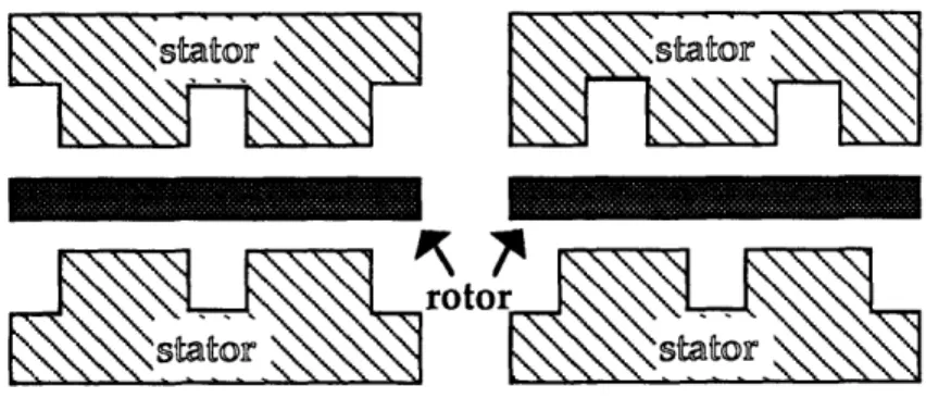
The authors of reference[6] through finite-element analysis techniques found that both tangential and axial components of torque ripple are effected by staggering one stator relative to the other (Figure 2.4).

_

_E~~~~~~~811

Figure 2.4: Unstaggered vs. Staggered Stators

Staggering the stators was found to greatly reduce the detent torque which resulted in smaller tangential torque ripple. However, staggering was found to cause much larger axial forces on the rotor. Additionally, it was found that axial forces are minimized when the stators are precisely aligned. Therefore, there is a trade-off between tangential and axial torque ripple components

when constructing a dual-stator axial-field motor. Both components can not be simultaneously minimized through construction techniques alone.

It is suggested in reference[6] that one choice is to build the motor with

precisely aligned stators to minimize axial torque ripple and then use

advanced control of the stator current waveforms to reduce the tangential

torque ripple. It may be possible to minimize axial torque ripple through

control of stator currents; however, this would required that separate current waveforms be applied to the two stators independently. Separate ports to the two stators are not usually provided making the latter suggestion impossible.

Therefore, the active reduction of the tangential component of torque ripple

only will be considered. It will be assumed from here on that the axial forces of the motor have been minimized through alignment of the two stators.

3 Active Torque Ripple Reduction Part I:

Current Selection

It was shown in Chapter 2 that unavoidable parasitics in stator and

rotor construction result in position dependent terms(i.e. torque ripple) when the stator excitation is a pure sinusoidal waveform. However, altering the stator excitation with harmonics at the appropriate frequency, amplitude, and phase can reduce the effect of the motor imperfections. The reduction of torque ripple through specific shaping of the stator excitation is termed Active

Torque Ripple Reduction (ATRR).

Assuming current mode control of the stator excitation essentially

removes the need to consider the stator or electrical dynamics when

analyzing the mechanical motor variables, it is beneficial to think of ATRR as

the active shaping of the stator current waveforms. Implicit in the current

shaping is the application of the appropriate stator voltages to generate the desired currents. This separation of variables suggests that there are two parts to ATRR-- selection of the appropriate current excitation to minimize the

torque ripple for the given motor at the given operating speed, and

enforcement of the selected current excitation through the application of the appropriate stator voltages to force the current to track the commanded

waveform. For many motors, including the dual air-gap axial-field PMAC

motor considered here, there is a significant time-scale separation between the electrical and mechanical dynamics(i.e. the electrical time-constants are much shorter than the mechanical). As a result, the controllers for each section can be designed separately and independently of each other. The remainder of Chapter 3 will consider the current selection problem. The current enforcement problem will be studied in Chapter 4.

3.1 Harmonic System Analysis

In order to select the appropriate stator current waveform to minimize torque ripple, it is first necessary to understand how a change in the stator current waveform affects the electrical torque waveform. A detailed motor

model including source of torque ripple was developed in Chapter 2,

to develop a systematic methodology for selecting the appropriate current waveform. As demonstrated by the simple example in Section 2.2, the

appropriate selection of current harmonics to cancel even a single inductance harmonic term required a clever guess for the form of the stator current. To solve the more general problem, a more precise analysis technique will be

required.

The reduction of torque ripple essentially means reduction of the non DC terms in the frequency spectrum of the electrical torque waveform. The pure time domain model derived in Chapter 2 does not provide the necessary

insight into the frequency response of the system. One method to gain this

insight is to introduce a transformation of variables in which the state-variables of the transformed system represent the frequency content of the system's physical state-variables. Consider the following nonlinear system

dx

-= f(x, U) (3.1)

dt

where x is the state-vector and u is the input vector, and whose state

trajectories exhibit periodic oscillations around their ideal(i.e. desired)

trajectories. Let the fundamental frequency of these periodic oscillations be co and define the following variable transformation.

o00O

x(t-T+s) =

£X

n(t)eJnW(t-T+s) (3.2)

n=-oo

u(t-T+s) = Un(t)ejn c(t-_{T+) (3.3)}

n=-oo

where T = 2n/w and se (O,T]. This transformation is in effect a time-varying Fourier Series expansion over the interval (t-T,t]. This expansion was used in reference [25] for use in the analysis of resonant power converters. A similar analysis will be applied here to the periodic oscillations of a rotating electric machine. The only assumption which need hold true is that the state-variable oscillations be periodic with the same fundamental frequency co, which is true

for the PMAC motor application. The transformed state-vector Xk(t) and

input-vector Uk(t) are complex functions of time. The original time functions x(t) and u(t) are real functions(i.e. a pure real number at each point in time)

which imposes the following constraints on the transformed state and input

variables,

X-n(t) = Xn(t)

Vn,t

(3.4)

U_n(t) = Un(t)

Vn,t

(3.5)

where X*(U*) is the complex conjugate of X(U). In the steady-state, the transformed variables Xk(t) and Uk(t) simply become the standard Fourier Series coefficients Xk and Uk,

00 x(t) =

YXne

jnwt (3.6) n=-oo 00oo u(t) = Unejnw (3.7) n=-oo

of the physical variables.

In many control schemes for rotating electrical machines, the control inputs are computed as functions of the rotor position 0 instead of time. This

approach is used because most state-variables in a rotating machine are

periodic in 0 with period 2, and 0 is a measurable quantity. The transformation of variables defined above can be modified to

x(0)=

IXn(t)ejn0

(3.8)

n=-oo

u(0) = ,Un(t)e ino (3.9)

n=-oo

In the steady-state, the rotor position 0 is proportional to time(i.e. 0=c0t).

Thus, the modified Equations (3.8) and (3.9) revert back to the original

transformation given by Equations (3.6) and (3.7) in steady-state operation.

The physical variables x(0) and u(0) are functions of position 0, but the

Fourier coefficients Xn(t) and Un(t) in equations (3.8) and (3.9) are still

functions of time. This implies that the control algorithm which will

compute the appropriate Un will be based on time. It is interesting to note that these Fourier coefficients could be taken to be functions of rotor position as

well(i.e. Xn(0) and Un(0) ), leading to a completely time independent

controller.

The transformation of variables given by Equations (3.8) and (3.9)

provides the type of system decomposition needed for the ATRR problem.

Note however that this transformation increases the order of the plant to

infinity. Even a simple first order system will require an infinite number of

state-variables in the transformed state-space. For the PMAC motor

application and most real systems, the bulk of the energy associated with the

state oscillations reside appears in a limited frequency band. For PMAC

motors, the torque ripple energy is concentrated around the fundamental

pole frequency of the machine. Thus, the number of Fourier coefficients required by the transformed system can be reduced by limiting frequency band of oscillations which will be considered. In this case, the transformation defined by Equations (3.8) and (3.9) changes to

N x(e) = XXn(t)ej n0 (3.10) n=-N N u(0) = Un(t)ejn0 (3.11) n=-N

which limits the order of the transformed system to 2N(i.e. the sum of the upper and lower summation limits from Equations (3.10) and (3.11)) and the highest considered oscillation frequency component to N times the rotor's rotational frequency co.

A second modeling problem exists with the transformation defined above. Consider the state of the system at time zero(i.e. t=0 and 0=0),

x(O) = XN()+...+X_ (0)+ X(O)+ X(0)+...+XN (0) (3.12) The initial state vector is easily converted to the transformed state-space, however, the mapping of the initial conditions to the new space is

under-constrained. This problem of mapping initial conditions through a variable

transformation is termed the initial condition problem. In general, the initial

condition problem may be over-constrained, one-to-one, or

under-constrained. In the under-constrained case, as in the PMAC motor

application, the problem becomes choosing the appropriate starting point to best represent the behavior of the physical system.

For a general system, the initial condition problem is non-trivial and

does not have a specific solution. However, for the synchronous motor

application, there is a solution which is better than the others. For an ideal

sinusoidal wound motor, the electrical states of the system(i.e. the stator

currents) are pure sinusoidal waveforms with the stator pole frequency(i.e.

Npco). Thus, one way to map the initial conditions on the electrical state-variables is to set the Np component equal to the given initial state with all other frequency components set to zero. This idea could be extended to an ideal square wound machine by setting the initial conditions at the frequency

components of the ideal input square wave currents. Also, in an ideal motor, the rotor speed co will have only a DC component in the steady-state(i.e. no ripple). Thus, it would make sense to map any initial rotor speed solely to its DC component in the transformed system. The second mechanical state, the rotor position 0, can be chosen to be zero initially. To summarize,

x(O) = X(O) + XNp (0) (3.13)

COO= COO + (3.14)

00N

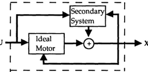
where io, coo, 00 are the initial stator currents, rotor speed, and rotor position respectfully. In essence, the system is modeled as an ideal PMAC motor which

is periodically disturbed by a secondary system causing the parasitic

oscillations at the overall system output(Figure 3.1).

, - - - -I

U X

Figure 3.1: TransformedSystem Block Diagram Figure 3.1: TransformedSystem Block Diagram

The initial conditions of the secondary system are assumed to be zero for

modeling convenience which is justified provided the contribution of

secondary system is much smaller than the ideal component(i.e. the motor is constructed well).

3.2 Harmonic Analysis of PMAC Motor

Using the background previously developed, the variable

transformation given by Equations (3.8) and (3.9) can be applied to the time domain state-space model for the PMAC motor developed in Chapter 2. The current control inner-loop that will be used to enforce the appropriate current waveform will be detailed in Chapter 4. Thus, it is justified at this level to consider the stator currents(i.e. ia, ib, and ic) as the control inputs, ignoring any stator electrical dynamics. It is necessary to choose current waveforms

with enough degrees of freedom to eliminate torque ripple due to both

inductance and cogging harmonics. The following choice provides the needed

freedom.

N N ia(o) = lm,nenN P (3.15) m=-N n=-N N N i0 n ib(O) = Imne (3.16) m=-N n=-N N N j(nNp-m 3)

ic(O)= Aj, ZimEne'm3 (3.17)

m=-N n=-N

where the Im,n's are the new control variables. In the steady-state, Im,n

represents the complex amplitude of the nth stator current harmonic with

phase offset multiple m where the fundamental frequency is the rotor's pole frequency, Np. The reasoning behind this choice of current excitation will be discussed further in this section.

The load torque Equation (2.10) of the motor also needs to be

transformed to the harmonic state-space since it is the load harmonic terms which need to be attenuated. Applying the variable transformation,

2N

TL(0) = XTnenNPO (3.18)

n=-2N

where Tn is the complex amplitude of the nth torque ripple harmonic. The summation limits in Equation (3.18) are correctly written as 2N (not N). It

will be shown shortly that N mutual inductance harmonics interacting with

N current harmonics can result in 2N torque harmonics.

The next step is to apply the harmonic variable transformation to the mutual inductance parameters of the motor as defined in Section 2.1(i.e. Lam, Lbm, and Lcm). N jnN 0 (3.19) Lam(0) LnenN P (3.19) n=-N N jn(NP0-3) (3.21) N -N Lm (0) = Lnej 3 (3.21) n=-N

Ln represents the complex amplitude for the nth inductance harmonic. For the ideal motor, the inductance terms will be pure sinusoids at the stator pole frequency, i.e.

Lm n =1

Ln l° else (3.22)

· =l"O~ n~else

For real motors, the inductance terms will contain higher order harmonics

which is one source of torque ripple, as mentioned in Section 2.2. In the worst case, all odd harmonics will be present with amplitudes decreasing inversely as the harmonic squared, i.e.

L

n odd

Ln =n (3.23)

0 else

For symmetry reasons, it will be assumed here that the harmonic content is the same for each phase(i.e. Ln is the same for Lam, Lbm, and Lcm). The variable transformation can also be applied to the cogging term Lmm,

2N

Lmm(O) = CneJnNP0 (3.24)

n=-2N

where Cn is the complex amplitude of the nth cogging harmonic. Keeping

with the symmetry assumption, the cogging is modeled as three equal

components, each contributing to a single stator phase. The fundamental

cogging harmonic will appear as the product of the stator and rotor pole frequencies. It is assumed here for simplicity that the stator and rotor pole frequencies are equal, however this is not required to perform this analysis.

The higher order cogging harmonics will be a function of the motor's

construction(teeth width, skewing angle, etc.) and may be estimated for a

specific motor either through experimental methods or finite element

numerical analysis techniques, see references [6] and [7].

Using the above computations, we can find the form of the electrical torque, Equation (2.17), in the transformed state-space. Since the electrical torque is a function of the derivatives of the inductance functions, the first step is to take the derivatives of Equations (3.19), (3.20), (3.21), and (3.24) with respect to 0. N dLm.= jnNpLnejnNP (3.25) dO n=-N dL N jn(N0 2) bm- j n N3 dOr j nNpLne 3 (3.26) n=-N dLcm

jjnnce

_Am=

jn(N 0-

_3(3.27)

) n=-N

2N

dLmm = 2nN nei P (3.28)

dO

_ jNpCe nNp_n=-2N 0

Substituting the stator currents, Equations (3.15), (3.16), and (3.17), and the mutual inductance derivatives, Equations (3.25), (3.26), and (3.27), into the mutual torque expression, Equation (2.20).

Ti.()km

Imne6

)(E

_

pLqe

JqNPo

T

+/(0)

km

=-N

n=-Nq=-N

Im,ne

jNpe

(3.29)

,=-Nn=-N q=-N

+kin j(nN -m 4-n N jq(N 0- 23)

+km

I

C

X

Im,ne

P

3

jjqNpLqe

lt

3

m=-Nn=-N

q=-This expression can be simplified by replacing the summation of summations terms by double summations.

) k

N

E

E

_ -j(m+n)

-i(n+q)N

+

-j(m+n)

4

3

Tg(0)=km I

Z

jqNpLqIme(n

q

)NO

(1

+e

+e

3

m=-N n=-N q=-N

A closer look at Equation (3.30), reveals that the mutual torque is simply a weighted convolution sum of the current and inductance harmonics. Notice from Equation (3.31) that the mutual torque harmonics are zero except when m+n is a multiple of three. The choice of n selects the frequency of the rotating magnetic stator field in the motor. The rotational frequency of the stator magnetic field is equal to nNpcw. The choice of m selects the direction of the rotating magnetic field. Choosing m to be in the set {1, 4, 7, ...} results in a positive rotating magnet stator field. Choosing m to be in the set 2, 5, 8, ...}

results in a negative multiple of three results in a negative rotating stator

field. Thus, this choice of input currents (i.e. Equations (3.15), (3.16), and (3.17) ) generates a linear combination of both positive and negative rotating fields at any desired frequency. By choosing the appropriate set of (m,n) [under the constraint that m+n is a multiple of three], it should be possible to generate rotating field components which cancel the rotating fields due to the parasitic inductance and cogging effects. This will result in torque ripple reduction.

Consider again the current waveforms, Equations (3.15), (3.16), and (3.17). Notice that, under the constraint that m+n is a multiple of three, these three-phase currents sum to zero for all 0, i.e.

ia(0)+ ib(0) + ic(0) = tVO (3.31)

Thus, this choice of current excitation may be applied to the Y-connected

motor configurations. A four wire or isolated winding configuration is not

required.

Substituting the cogging inductance derivative, Equation (3.28), into the cogging torque expression, Equation (2.39), yields

2N

Tc(0) =k2m jnNpCneinNP (3.32)

n=-2N

The sum of the mutual torque, Equation (3.30), and the cogging, Equation (3.32), is the total torque of electrical origin. In the steady-state, the total electrical torque must equal the load torque, i.e.

Tt(0) = T, (0) + TC(0) = TL(0) (3.33)

Using the above results, the complete torque balance equations in the

harmonic state-space become

k N CNpL q)m e-j(m+n)- -j(m+n)- km jqN Ll j(n+q)NPO(1+ e +e ) m=-N n=-N q=-N (3.34) 2N 2N +k2 _{CjnNpCneinNe ETneJNp} n=-2N n=-2N

This equations contains a large quantity of information. It shows how the

inductance, current, and cogging harmonics combine to create torque

harmonics. In addition, Equation (3.34) shows explicitly how to compute the complex weighting factors which when combined determine the magnitude and phase of the torque ripple.

To gain further insight, the torque balance relation, Equation (3.34), can be written in a matrix form.

LI + C = T

where L, I, C, and T take on the following forms.

... n+q=O ... n+q=l ... n+q=2 ... n+q=2N ...

(3.36) I =

I-N-N

I-m,-n Im,n IN,N

-N<m<N

-N < n <N (3.37) m + n is a a multiple of 3. 0 To C, T, C =

1

(3.38) T= 1 (3.39)

The dimension of L is 2N+1 by (2N)2/3, I is (2N)2/3 by 1, C is 2N+1 by 1, and T is 2N+1 by 1, thus Equation (3.35) is dimensionally correct. Notice that N

current harmonics and N mutual inductance harmonics can produce 2N

torque harmonics. This is due to the convolution relationships, and in

general, the total number of torque harmonics will be the sum of the number

of current harmonics and mutual inductance harmonics. Since m+n needs to

be a multiple of three to produce an effect on the torque harmonics(see Equation (3.34) ), current harmonics in which m+n is not a multiple of three should be set to zero. They do not contribute to torque ripple reduction and result in resistive losses. As such, N should be chosen to be a multiple of 3 to insure that I-N,-N and IN,N (i.e. the first and last terms in Equation (3.37)) effect torque ripple.

If the mutual inductance matrix L and the cogging spectrum C for a motor is known precisely, the minimum torque ripple current excitation can be computed by solving the linear system of equations(i.e. Equation (3.35) ). The mutual inductance L will contain more columns than rows for any choice of N (integer). Therefore, the system of equations is under-constrained

(i.e. there exists many current vector I which satisfy the matrix equation). We

(3.35)

are free to choose any solution we wish. It makes sense to choose the solution which minimizes the I2R losses in the motor windings, and thus, maximizes efficiency. Minimizing I2R losses is equivalent to minimizing the norm of

the vector I (see reference [3]). The minimum norm solution of Equation

(3.35) is given by the following,

I =(L*L)-lL*(u

C)

-

(3.40)

where L* is the complex conjugate of the matrix L and u contains the Fourier coefficients of the desired torque spectrum.

U =[ T (3.41)

To eliminate torque ripple, the commanded torque spectrum should only

contain a DC component, i.e.

To

u=O (3.42)

where T is the commanded torque which may be set by an outer speed control loop.

The above discussion shows the value of using this harmonic

decomposition analysis. Given a motor's mutual inductance and cogging

coefficients, the L matrix and C vector can be computed, and the optimal current coefficients I to eliminate torque ripple can be found. Unfortunately, this is not the end of the problem. The inductance and cogging parameters are not easily measurable off-line. In addition, they may change slightly over the operational life-time of the motor. Therefore, a fixed implementation of Equation (3.40) does not constitute a reliable solution to the problem. An adaptive control approach which uses Equation (3.40) as a basis and provides a more robust solution will be presented in Section 3.3.

3.3 Minimum Torque Ripple Current Controller

The analysis in Section 3.2 provides insight into the source of

tangential torque in PMAC motors. It shows that torque harmonics can,

theoretically, be controlled (or eliminated) through the careful addition of harmonic terms to the stator current waveforms. Equation (3.40) shows how

to compute the amplitude and phase of the required current harmonics to

impose a desired torque spectrum with maximum efficiency. This

computation requires explicit knowledge of motor parameters(i.e. the

matrices L and C). Unfortunately, the control calculation is sensitive to errors in these parameters. To use this control scheme in a practical motor drive, it would necessary to correct for these errors. One method for dealing with the sensitivity issue is to use adaptive control.

Speed Control Loop

Torque Control Loop

I r - .t _ - 1 Oref °t I V V . V L I I I I I I I I II

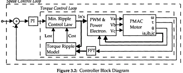
Figure 3.2: Controller Block Diagram

Figure 3.2 shows a Model Reference Adaptive System (MRAS)[28]. The control system is composed of two loops. The outer speed loop controls the commanded torque to regulate the shaft's rotational speed. The inner torque loop controls the applied current waveform to impose the desired working

torque without ripple harmonics. The essential idea of the torque control

loop is to use measurements of the torque ripple spectrum to recursively

estimate the inductance and cogging harmonic terms( i.e. L and C from

Equation (3.40) ). The estimates of these parameters will be referred to as Lest and Cest. Using these estimates, the appropriate current harmonics required to impose the desired DC torque with minimal ripple terms can be computed.

The first step to implementing the MRAS system shown in Figure 3.2

is to derive an parameter estimation process. The model given by Equation

(3.34) provides the necessary basis. It is a given that the cogging torque can not have a DC component(i.e. Co=O). Therefore, it is guaranteed that the DC equation of (3.34) is can be written as the inner product of vectors containing

the mutual inductance and current coefficients, i.e.

TO= [I-N,-N ... I0,0 ... IN,N] LN ... Lo L...N _L-N_ (3.43)

Given that the DC inductance component L must also be zero, and all other Fourier coefficients must appear as complex conjugates, Equation (3.43) can be reduced to

2 = [I-N,-N ... Il .. (3.44)

2

Since Equation (3.44) is linear, it is possible to apply least-squares (LS)

techniques[28] to provide estimates of the inductance parameters given

measurements of the DC torque which can be computed from a shaft speed measurement( see Equation (2.28) ). To describe the LS update law, it is first necessary to define the following quantities:

0(t) = .... (3.45) I - N_,- N (p(t) = ... (3.46) y(t) 2 (3.47) y(t) T O (3.47) 2

where t is an index representing the current time step. One method for

recursively computing a least-squares parameter estimate is Kaczmarz's

algorithm[28]. Using the parameter definitions given by Equations (3.45), (3.46), and (3.47), an estimate of the inductance parameters 0(t) may be computed as follows

0(t) = 0(t -1) + (PT [y(t)- (pT0(t - 1)] (3.48)

a+

(pp

where 0(t) is the best least-squares estimate of the inductance parameters

given the previous estimate 0(t-1) and the most recent output measurement

y(t). Motor back EMF measurements may be used to provide an initial

parameter estimate 00 which assumes no parasitic inductance harmonics,

Go =

i

(3.49)

Eb

where, L (3.50)

If back EMF data is not available, the estimate may be initialized to zero. The later case will result in a slower parameter convergence. The variables ca and

in Equation (3.48) are estimator design parameters. a should be a small

positive number whose purpose is to prevent the estimate from diverging

when the input vector (p becomes very small. y is the estimator's gain whose value represents a trade-off between convergence rate and stability. A large gain will result in fast parameter convergence, however, for a large enough gain the estimator will become unstable. As indicated in reference[28], the gain should be chosen between 0 and a maximum of 2 to prevent instability.

The Kaczmarz algorithm is a good estimator choice for motor drive

applications due to its simplicity of implementation and speed of

computation.

Both are important constraints in motor drive

implementations. Other least-square algorithms, such as Gauss[28], boast

faster convergence rates, however at the expense of greater computational complexity.

One caution should be mention concerning the use of any recursive least-squares algorithm. In order to estimate a system parameter from the

output measurements, it is necessary that the mode associated with that

system parameter is excited by the input and observable in the output. This

constraint is called the Excitation Condition. For the Kaczmarz estimator

described above, the excitation condition can be described as follows. Define the matrix D such that,

I) = (pPT (3.51)

where c( was defined in Equation (3.46). The excitation condition is satisfied provided the matrix D has full rank. This result has an physically intuitive interpretation for the motor application. Considering Equation (3.44), the DC

electrical torque component is the result of each inductance harmonic

multiplied by its corresponding current harmonic. To estimate the nth

inductance harmonic Ln, the input current waveform must include the nth

current harmonic In. To make sure that all desired inductance harmonics are

present in the output, it is recommended that all current harmonics be

initialized to some non-zero quantity. This is equivalent to forcing the input

matrix(i.e. Equation (3.51) ) to have full rank.

Given the parameter estimate 0(t), the inductance matrix estimate, Lest, can be constructed and used to estimate the cogging spectrum Cest.

Cest = T - LestI (3.52)

With the inductance and cogging harmonic estimates, Lest and Cest, the

current control law which results in minimum torque ripple can be defined as follows.

I = (LestLest )- Lest(u - Cest) (3.53)

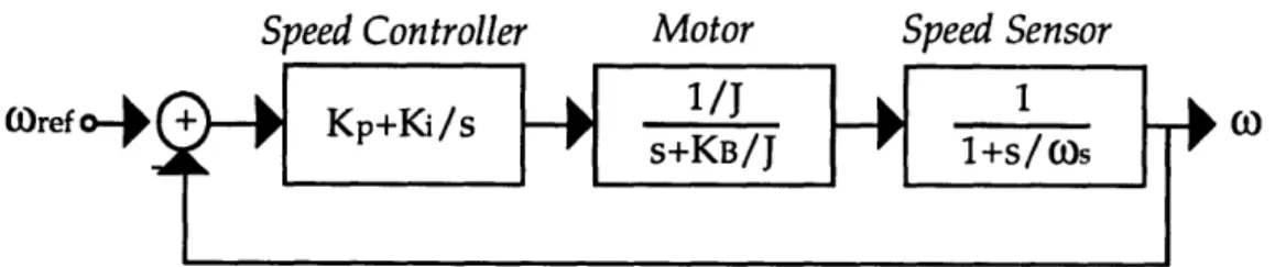
One beneficial feature of the MRAS system shown in Figure 3.2 is that the inner torque control loop may be considered as transparent to the outer speed loop. Thus, the gains of the speed tracking PI compensator may be designed independent of the inner current control law.

(Oref o-

Figure 3.3: Speed Controller Transfer Function Diagram

where J and KB are the moment of inertia and load damping coefficient for

the motor and propulsor respectively, Kp and Ki are the speed controller

gains, Cos is the 3 dB bandwidth of the speed sensor. Using Figure 3.3, the speed input-output transfer function can be derived.

co 1 Kps + Ki

=_ (3.54)

coref J s(s+ K)( S +1)

J oS

Thus, the poles and zeros of the motor's speed dynamics are simply functions

the motor's parameters, speed loop controller gains, and speed sensor

characteristics. They do not influence torque ripple with the given setup. The power electronics and FFT subsystems will be discussed further in Chapters 4 and 5 respectively. The next section will provide some computer

simulation results of the parameter estimate and current control law

subsystems.

3.4 Harmonic System Simulation & Parameter Estimation

The following computer simulations of the motor model and

controller described above were constructed using SIMULINK[29]. They are

intended to show the validity of the torque ripple model developed in

Section 3.2 and demonstrate the performance of the parameter estimator

developed in Section 3.3. This simulation deals only with the transformed Fourier state-variables as they are defined by Equations (3.15) through (3.21).

A more detailed simulation which is based on the motor's physical

state-variables will be presented in Chapter 6.

Torque Constant Cogging Coefficient Max Current Amplitude Moment of Inertia Damping Coefficient Number of Pole Pairs

Lmm Imax J Bco Np 0.1 150 0.2 0.1 24 H A kg m2 2 NM/RPM

Table 3.1: Simulation Parameters

Nominal parameters for a dual stator axial-field PMAC motor were

used and are shown in Table 3.1[6]. Graph 3.1 shows the rotor's velocity

profile. In this test, the motor was given a 100 RPM step velocity command

from rest. As shown, the rotor responded with a slightly under-damped

response, a 2 second rise time, and zero steady-state error. As noted

previously, the rotor's response is dictated completely by the choice of gains for the outer speed control loop( see Figure 3.3 ) and is does not affect torque

ripple.

Graphs 3.2 through 3.7 show the magnitude and phase of the first 6

harmonics of the resulting torque ripple. Only the initial adaptation phase

(i.e. open-loop system) is demonstrated here.

Graph 3.8 shows the applied current harmonics to the system during

this initial adaptation phase. It should be noted that since only the first 6

torque harmonics are considered here, it is necessary to applied up to the

third current harmonic.

Graphs 3.9 and 3.10 shows the computed estimates of inductance and cogging harmonics, respectively. The real values are shown as dashed lines on these graphs. As expected, each estimate converged in the steady-state to

the true parameter value.

.

NM/A