Benchmarking convolutional neural networks for object segmentation and pose estimation

Benchmarking Convolutional Neural Networks for

Object Segmentation and Pose Estimation

by Tiffany Anh Mai Le

S.B., Massachusetts Institute of Technology (2016)

Submitted to the

Department of Electrical Engineering and Computer Science

in partial fulfillment of the requirements for the degree of

Master of Engineering in Electrical Engineering and Computer Science

at the

Massachusetts Institute of Technology

September 2017

c

Tiffany Anh Mai Le, 2017. All rights reserved.

The author hereby grants to MIT and The Charles Stark Draper

Laboratory, Inc. permission to reproduce and to distribute publicly

paper and electronic copies of this thesis document in whole or in any

part medium now known or hereafter created.

Author . . . .

Department of Electrical Engineering and Computer Science

August 17, 2017

Certified by . . . .

Lei Hamilton

Senior Member of Technical Staff, Draper Laboratory

Thesis Supervisor

Certified by . . . .

Antonio Torralba

Professor of Electrical Engineering and Computer Science

Thesis Supervisor

Accepted by . . . .

Christopher Terman

Chairman, Masters of Engineering Thesis Committee

Benchmarking Convolutional Neural Networks for Object

Segmentation and Pose Estimation

by Tiffany Anh Mai Le

Submitted to the Department of Electrical Engineering and Computer Science on August 17, 2017, in partial fulfillment of the

requirements for the degree of

Master of Engineering in Electrical Engineering and Computer Science

Abstract

Convolutional neural networks (CNNs), particularly those designed for object seg-mentation and pose estimation, are now applied to robotics applications involving mobile manipulation. For these robotic applications to be successful, robust and accurate performance from the CNNs is critical. Therefore, in order to develop an understanding of CNN performance, several CNN architectures are benchmarked on a set of metrics for object segmentation and pose estimation. This thesis presents these benchmarking results, which show that metric performance is dependent on the complexity of network architectures. The reasons behind poor pose estimation and object segmentation, which include object symmetry and resolution loss due to downsampling followed by upsampling in the networks, respectively, are also identi-fied in this thesis. These findings can be used to guide and improve the development of CNNs for object segmentation and pose estimation in the future.

Thesis Supervisor: Lei Hamilton

Title: Senior Member of Technical Staff, Draper Laboratory

Thesis Supervisor: Antonio Torralba

Acknowledgments

I would first like to thank my advisers, Lei Hamilton and Antonio Torralba, for their invaluable guidance and mentorship in the writing of this thesis. I greatly appreciate all of the time, effort, energy, and patience that they have put in throughout this entire process.

I would also like to thank Dave Johnson and the Draper Laboratory Autonomy Inter-nal Research and Development (IRAD) Team for all of their help whenever I needed it, including, but not limited to data set collection and labeling, and code debugging.

Next, I would like to thank Draper Laboratory and the Draper Fellows Program for granting me the fellowship that sponsored this research, thus providing me with this research opportunity.

Finally, I would like to thank my friends and family for their support throughout the years, particularly this past year, as I was writing my thesis. I would especially like to thank my parents for their unconditional love and for always being there for me.

Contents

2.2 SegNet . . . 24

2.3 PoseNet . . . 26

2.4 FuseNet . . . 27

2.5 Generative Adversarial Networks . . . 28

3 Benchmarking Framework 29 3.1 Framework . . . 29 3.2 Data . . . 30 3.3 Training . . . 33 3.4 Testing . . . 34 3.5 Benchmarking Metrics . . . 35

4 Results 39

4.1 Segmentation Results . . . 39

4.2 Segmentation Metric Comparisons . . . 43

4.3 Robot Performance Comparisons . . . 48

4.4 PoseNet Pose Estimation Results . . . 50

5 Conclusions 53 5.1 Summary . . . 53

5.2 Future Work . . . 54

A Data Set Pose Distribution 57

List of Figures

1-1 Oil Change Task . . . 15

1-2 Semantic Segmentation . . . 15

1-3 Segmentation and ICP Point Cloud Alignment Process . . . 16

2-1 Max and Average Pooling . . . 22

2-2 SegNet Architecture . . . 25

2-3 PoseNet Architecture . . . 26

2-4 FuseNet Architecture . . . 27

2-5 SegNetGAN Architecture . . . 28

3-1 Sample Data Set Elements . . . 31

3-2 Object Classes . . . 31

3-3 Data Set Object Distribution . . . 32

3-4 Roll Pitch Yaw Representation . . . 33

3-5 Confusion Matrix . . . 36

4-1 SegNet Segmentation Results . . . 40

4-2 SegNetGAN Segmentation Results . . . 40

4-3 FuseNet Segmentation Results . . . 41

4-4 PoseNet Segmentation Results . . . 41

4-5 Per Class Accuracy . . . 44

4-6 Per Class IOU . . . 44

4-7 Per Class Recall . . . 44

4-9 Robot Performance Comparisons . . . 49 4-10 PoseNet Pose Projection Results . . . 52

List of Tables

3.1 Training Parameters . . . 34

4.1 Summary of Metrics . . . 45

4.2 Summary of Per Class Accuracy . . . 45

4.3 Summary of Per Class IOU . . . 46

4.4 Summary of Per Class Precision . . . 46

4.5 Summary of Per Class Recall . . . 47

Chapter 1

Introduction

Humans are constantly trying to understand their surroundings, particularly through visual cues, in everyday life. Beyond just being able to have a visual understanding of their environment, humans also interact with and manipulate objects in the real-world environment. This visual perception of the environment may include identifying and recognizing the scene along with the objects in it, localizing these objects in space, and, if necessary, navigating around the environment to get close enough to manipulate a desired object. While these tasks come easily and naturally for humans, they are currently much harder for robots to do. In order for robots to accomplish these same tasks, robots must mimic the way that humans visualize and perceive their environment. Conventionally, this manner of robotics perception entails utilizing sensors to capture a visual of the scene, in the form of a two-dimensional (2D), three-channel red, green, blue (RGB) color image and a depth map. Following the capture of the sensor data, computer vision is used for object detection and segmentation. In the field of computer vision, convolutional neural networks (CNNs) have recently become a breakthrough method of object detection [13]. In recent years, the increased popularity and use of CNNs have resulted in greater performance gains in object classification, recognition, and segmentation, among other tasks. In fact, in some cases, CNNs can perform as well as, and even outperform humans [17]. Current applications that use CNNs for robotic perception include autonomous vehicles for navigation, road detection, and obstacle avoidance as well as automation of assembly

lines for parts assembly and product quality control.

1.1

Mobile Manipulation

Mobile manipulation is an important component of robotics applications, enabling the robot to perform human-level tasks involving physical interaction with the envi-ronment. One application that showcases the tasks involved in mobile manipulation and robotics perception is the motorcycle engine oil change task, as performed by an autonomous robot. The autonomous oil change process can be broken down into a planned sequence of several key steps for adding new oil to the engine, with perception playing a key role along each step of the way in the execution. First, the engine must be identified, in particular the cap on top of the engine oil port. Subsequently, the robot must remove the cap from the oil port. After completing these steps, a funnel must be located and be picked up by the robot. Following this, the robot inserts the funnel into the engine oil port, as depicted in Figure 1-1. Next, the oil bottle must be detected and the oil bottle cap must be removed by the robot. The robot then picks up the oil bottle, and returns to where the funnel and engine are located. At this point, the bottle is tipped to pour oil into the funnel. Once the pouring is complete, the oil bottle is returned to its original location and the oil bottle cap is replaced on the oil bottle. To finish the oil change, the funnel is removed from the oil port and the engine oil cap is placed back on the engine. Overall, because of the numerous steps and objects involved in the oil change process, with each of the objects needing to be manipulated in different ways, such as grasping, twisting, or turning, the entire oil change process is particularly complex to complete.

To accomplish these tasks, robotics perception systems utilize CNNs for semantic segmentation, which classifies every pixel of an image into a given set of identifiable objects and regions. Figure 1-2 shows an example of this, with the original image in 1-2a and the corresponding semantic segmentation in 1-2b. Each of the different white regions in 1-2b corresponds to a different class of interest and encompasses the

Figure 1-1: Oil Change Task - As one step in the Autonomous oil change task, the robot inserts the funnel into the engine.

entire area corresponding to that class in the original image.

(a) Original Image (b) Segmented Image

Figure 1-2: Semantic Segmentation - An original scene and the corresponding semantic segmentation with the objects of interest labeled.

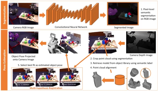
Using this segmentation information, along with the scene depth information, robotics perception systems are then able to take advantage of algorithms, such as Iterative Closest Point (ICP). ICP is used to align a previously generated 3D model of the object taken from a database of object models with a view of the segmented object point cloud and find the best match between the two [22]. Based on this alignment, object pose estimates are generated. Object pose, which not only describes the ob-ject’s position in space, but also the obob-ject’s orientation, is crucial in informing the

robot about the location of an object and how to adjust its arm to manipulate the object. Figure 1-3 shows the segmentation and alignment process. A 2D segmented image is generated by a CNN, which is then used to crop the point cloud associated with the object of interest, and align this point cloud with a 3D object model. From this, the best alignment is used as an estimate of the object pose, providing an initial target that the robot uses to manipulate the object.

Figure 1-3: Segmentation and ICP Point Cloud Alignment Process - This method estimates object pose by using a segmented image for point cloud alignment.

While generally effective, some challenges still remain in the mobile manipulation process [11]. First, a major difficulty that mobile manipulation systems face is that environments are commonly unstructured so scenes can be extremely varied and clut-tered, particularly indoors. This makes it difficult for a robot to consistently recognize the same object from scene to scene. Furthermore, objects of interest in the scene may be occluded by other objects. Secondly, even without occlusion, a single object can have different physical properties and geometries, resulting in changes in object appearance depending on the viewpoint. In fact, this variation in object appearance makes it difficult to associate specific features with an object that is necessary for

reliable object identification, as different objects may look like the objects of interest, resulting in false identifications. Third, as the robot is moving in mobile manipula-tion, the scene is now no longer static. This movement is problematic, since not only can objects now move in and out of the field of view of the robot, but the scale of the given objects also changes in size depending on the distance that the robot moves away from or towards the objects. Finally, pose alignment difficulties can arise, as a result of poor segmentation performance, since the segmented object point cloud and the 3D object model need to match in order to get a correct initial registration for pose estimation. However, a good fit between the segmented point cloud and the 3D model is not always possible as the object segmentation may not provide enough information about the object in order to generate the fit, if the object is reflective, concave, too far away from the sensor, or only a small portion of the object is visible in the camera frame, for example. In these cases, human involvement is required to move the object close enough to the sensor or place it at a different angle for the estimation to be effective, further motivating the need for good object segmentation in an autonomous system. In general, with all of these difficulties in the mobile ma-nipulation process, the purpose of this thesis is to understand and improve object segmentation and pose estimation performance.

1.2

Thesis Contributions

To address the difficulties with object segmentation and pose estimation, machine learning is used to enhance robotics perception [11]. In particular, CNNs have made rapid progress and are now the standard practice in the fields of machine learning and computer vision. Moreover, CNNs have been recognized for recent successes in learning, with regards to object detection for a wide range of tasks and applications. However, even with the success of many different CNNs in aiding robotics perception, there are still gaps in the understanding of CNN performance and how this perfor-mance translates to robotic perforperfor-mance. In light of these gaps, and in an effort to address some of the current difficulties in robotics perception, particularly within the

autonomous motorcycle engine oil change context, as part of the ongoing research at Draper on mobile manipulation, this thesis focuses on benchmarking metrics for both object segmentation and pose estimation, since having both components will provide a better overall understanding of the object for the robot. Specifically, the major contribution of this thesis is the development of the specific benchmarking function-ality built upon a testing and training framework for CNNs. Using the framework, this thesis benchmarks a set of CNNs on a range of metrics to compare and analyze CNN performance in an objective way to determine correlations between metric per-formance and specific CNN architectures. Furthermore, this thesis identifies factors that contribute to both high and poor performance in CNNs, which can be used to develop and improve networks that will provide more reliable object segmentation and pose estimation in the future. Finally, because robot performance relies on having robust object segmentation and pose estimation, this work investigates what metrics are best to evaluate the performance, particularly with respect to how these metrics relate to performance on the robot.

The background of this thesis is described in Chapter 2, which includes topics such as CNN architectures, along with previous research that this thesis builds upon. In Chapter 3, the benchmarking framework will be introduced, with emphasis on dataset generation, the framework functionality, along with training and testing procedures. Next, Chapter 4 will present the results and provide a discussion of the results. Finally, Chapter 5 will summarize the work done in this thesis.

Chapter 2

Background

Robotics perception is accomplished using CNNs for object detection. The use of CNNs is a result of recent advances in hardware and availability of large data sets that have allowed CNNs to become more feasible, and therefore, more widely used, resulting in major performance gains in object recognition and segmentation. Prior to the use of CNNs, object detection was dependent on hand-engineered feature de-scription algorithms such as Scale Invariant Feature Transform (SIFT), Speeded Up Robust Features (SURF), and Histogram of Oriented Gradient (HOG) [2, 5, 15]. These methods calculate gradients around points of interest to be used for matching to the objects of interest. However, the handcrafted features derived from these al-gorithms have limited performance [2]. In contrast, with the rapid development of CNNs, performance has been able to improve significantly, even surpassing human accuracy on some classification tasks.

For robotic applications, not only is object segmentation important, but pose esti-mation is also a critical component. While prior work on pose alignment focuses on putting markers on the objects for robots to recognize and locate objects, nowadays, systems without markers have been introduced [4]. The markerless pose alignment systems generally involve the use of algorithms such as ICP to match with a 3D model. However, the development of CNNs to estimate pose has provided another alternative method for pose alignment.

This thesis will leverage and extend the currently existing work with CNNs with regards to object segmentation and pose estimation in an attempt to evaluate their performance. Overall, this thesis aims to evaluate several CNNs designed for object segmentation and pose estimation to determine which network architectures may provide high performance. An overview of CNN architectures along with the CNNs of interest that are investigated further in this thesis for their performance in object segmentation and pose estimation tasks are introduced and described in this chapter.

2.1

Overview of Convolutional Neural Networks

CNNs are a cascade of layers with each layer generating an abstract representation of input through a transformation that is applied at each of the interconnected layers. CNNs are inspired by the human brain and the way that the human brain processes visual information. The primary feature of CNNs are the convolutional layers that make up the network. The convolutional layers are filters that act upon the input image x in a pixel-wise manner to produce an output y, at a given pixel position (i, j), as defined in Equation 2.1. Each of these filters, of size M by N , has a set of associated weights, W , and biases, b, corresponding to the parameters that the network learns. yi,j = ( M/2 X m=−M/2 N/2 X n=−N/2 Wm,n· xm+i,n+j) + b (2.1)

Each convolutional layer produces feature maps through convolution of input with the filter in the associated layer. There are different levels of abstraction for the output feature maps depending on where the convolutional layer is in the network. Lower level semantic features such as edges or colors are closer to the input layer, while mid to high level semantic features such as object parts or entire objects themselves can be determined near the output at the later layers. Moreover, these convolutional layers can be fully-connected, which connects the output in the current layer to every

output of the previous layers. These connections allow the network to learn varied combinations of features.

Besides the convolutional layers, additional layers are used to compose a CNN, with each of the layers contributing in different ways to transforming the resulting network output. Some of these common layers include pooling layers, unpooling layers, batch normalization layers, dropout layers, linear layers, as well as activation layers.

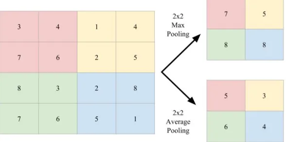
Pooling layers are used to downsample the input, reducing the number of network computations [19]. Furthermore, this downsampling reduces the feature map resolu-tion. With the lower feature map resolution, spatial feature invariance is improved, making the network more robust due to translational shifts. Commonly used pooling functions include max pooling and average pooling [14]. While the max pooling func-tion finds the largest value of the input subregion selected by the pooling window, the average pooling window calculates the mean value found in this region. Figure 2-1 shows an example comparison between the results of max and average pooling on a given input region.

Unpooling layers perform the approximate inverse function of the pooling layers by upsampling the input [24]. Each unpooling layer has an associated pooling layer, from which the pooling indices are taken. This is useful to reconstruct the original structure of the input features to the pooling layer.

Batch normalization layers compute a normalized output, ˆx(k), for each dimension, k, of the layer input, x as shown in Equation 2.2, where E[x(k)_{] and V ar[x}(k)_{] are the}

mean and variance computed over the training data set, respectively [10]. This nor-malization is done before the activation layers to stabilize the activation distribution and act as a regularizer. The regularization allows for much higher learning rates to be used in training, with less emphasis needed on the initialization of weights, while improving accuracy and convergence time.

Figure 2-1: Max and Average Pooling - A comparison between downsampling an input region using 2x2 Max Pooling vs. 2x2 Average Pooling.

ˆ

x(k) = x

(k)_{− E[x}(k)_]

p

V ar[x(k)_] (2.2)

Dropout Layers are similar to batch normalization layers, in that dropout layers also work to regularize the neural network [21]. However, dropout layers do this regularization by adding noise to the units in the neural network layer, and randomly removing some of these units and all of the connections, both input and output, from the network, with a probability, p, temporarily. The removal of the units additionally helps to prevent overfitting of the network.

Linear layers apply a linear transformation to the input, x, by scaling the input by A, and shifting this scaled input by b, shown in Equation 2.3. This linear transformation makes it suitable for linear regression, as it maps the input dimension to a given output dimension, enabling prediction of the output from the input.

Activation layers perform an operation on the input, resulting in a binary response of whether to trigger at the output, based on whether the input exceeds a given threshold value. One particular activation layer of interest is a Rectified Linear Unit (ReLU) layer, which introduces a non-linearity by performing a thresholding activa-tion funcactiva-tion on the input, as defined in Equaactiva-tion 2.4, for an input, x. This removes all negative input values, thus only activating the specific features of interest, and improves convergence.

RELU (x) = max(0, x) (2.4)

Another activation layer of interest are Exponential Linear Unit (ELU) layers. The ELU function is similar to the ReLU function, but can have negative values, which is controlled by setting α, for the input, x, as defined in Equation 2.5 which allows for better network generalization and faster learning, as compared to ReLU [3].

ELU (α, x) =      α(exp(x) − 1) if x ≤ 0 x if x > 0 (2.5)

Softmax layers are a third activation layer of interest. They are used for multiclass classification, to predict the probability that the output, y, is of a given class k, provided the input x and w, the sum of the weights, for each of the N classes, as defined in Equation 2.6 [6].

P rob(y = k|x) = exp(wkx) PN

n=1exp(wnx)

(2.6)

A final activation layer of interest is the Sigmoid activation layer, where the Sigmoid function is as defined in Equation 2.7. The Sigmoid activation layer is commonly used because of the smoothness and simplicity of the derivative of the Sigmoid function, which is critical in neural network backpropagation for optimization of the network

weights. Moreover, because the Sigmoid function ranges from 0 to 1, this activation layer is often used to represent the probabilities in a binary classifier.

Sigmoid(x) = 1

1 + exp(−x) (2.7)

When building CNN architectures by combining these different network layers, major improvements in CNN performance have been attributed to appending additional convolutional layers to basic network architectures, resulting in the creation of deeper CNNs. The relationship between the depth of a CNN and its performance has been studied through the development of VGGNet, showing that deeper networks result in higher accuracy for image classification tasks [20]. Moreover, this high performance from deep networks can be extended to other object recognition or localization tasks as well. Based on a standard CNN architecture, which traditionally has fewer than five convolutional layers, VGGNet extends the number of convolutional layers to form a 19-layer network. However, several modifications were made to compensate for the added network depth. VGGNet uses small 3x3 filters, to keep the number of weights less than that of a shallower CNN architecture, but with larger filter sizes. Additionally, because random initialization of the weights in each layer can result in instabilities when training, VGGNet initializes the first few and last few layers with pre-trained weights, and only randomly initializing the layers in the middle. With these modifications, VGGNet was able to improve and provide state-of-the-art classification accuracy due to the regularization gained from having the additional layers. As an added benefit, the depth of the network enables it to generalize well to a variety of tasks and data sets, resulting in the use of VGGNet as the basis for many other deep CNNs.

2.2

SegNet

One network that is based on VGGNet is SegNet, which performs pixel-wise semantic segmentation in an efficient manner [1]. SegNet differs from VGGNet due to the

removal of the fully-connected layers from the network architecture. This results in SegNet consisting of only 13 encoder layers, and a corresponding decoder layer for each encoder layer, for a total of 13 decoder layers. This was done in an attempt to make the network smaller and therefore, easier to train. Each encoder consists of a convolutional layer, a batch normalization layer, and a RELU layer. Max-pooling layers are interspersed throughout the encoder architecture, placed after every three or four encoder layers. The decoder uses the max-pooling indices to undo the effects of the downsampling and upsample the feature maps. There is no learning in this upsampling process, however, so following the upsampling, trainable decoder filters are convolved with the upsampled feature maps to generate full output feature maps. Consequently, the use of the max-pooling indices in the decoder reduces the amount of information that needs to be stored, with minimal impact on performance. The final decoder produces a multi-channel feature map, with the number of channels corresponding to the number of objects to be classified. The final soft-max layer acts as the object classifier, predicting class probabilities for every pixel in the image. SegNet currently performs well on object segmentations, even in indoor scenes, so this thesis seeks to extend upon this work, by applying it to the oil change context, as well as develop several other architectures off of this network to determine if these modified architectures can yield improvements in object segmentation.

Figure 2-2: SegNet Architecture - The neural network layers forming the encoder-decoder structure making up SegNet. The network takes in an RGB input

2.3

PoseNet

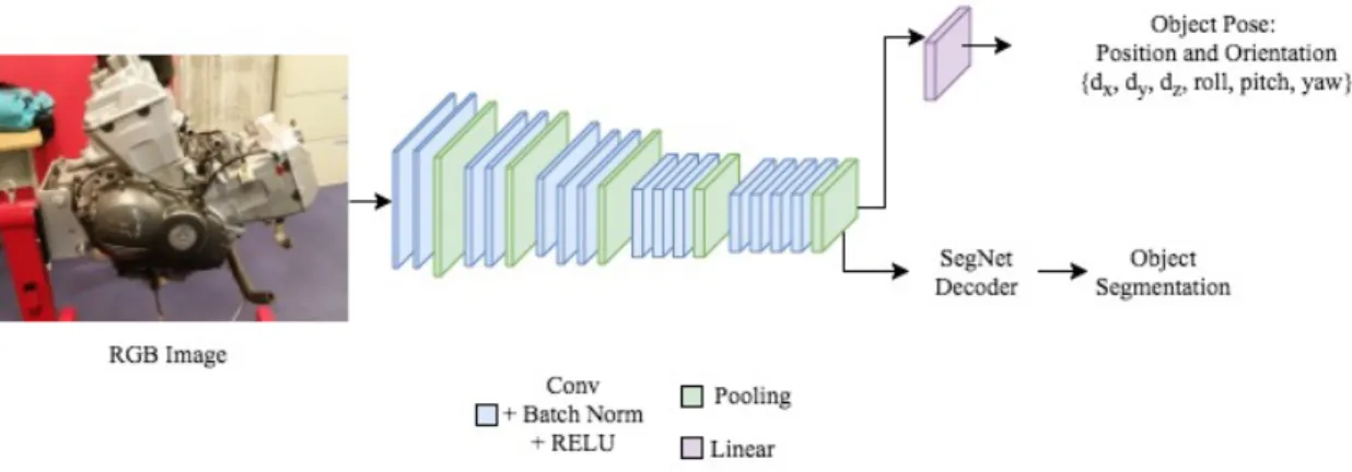
Figure 2-3: PoseNet Architecture - The neural network layers forming the two branches of PoseNet. The network takes in an RGB input and produces both an

object segmentation and a pose estimate at the output.

CNNs have also been used for applications extending beyond image classification. One such application is the development of a CNN to estimate the camera pose of an object directly from an image. Object pose is defined by an orientation, which is the angle at which an object is tilted or rotated in the camera view, and position, which corresponds to the object location mapped from the 3D world to the camera view. One implementation of a CNN for camera pose estimation is PoseNet. PoseNet regresses an objects pose from a pre-trained classifier, leveraging transfer learning from the classification data [12]. It has 23 layers, which allows it to learn high level features, while making it robust to lighting, motion blur, and camera properties. Moreover, very few training samples are needed for convergence, with meter level accuracy for position coordinates, and within 2-5 degrees for angle approximations. Based on this idea, and in order to be able to compare object segmentation metrics between models, we create a modified version of PoseNet 1_{. We use the SegNet}

encoder and decoder, but just before the final fully-connected layer of the SegNet encoder, we add a linear regression layer. This results in a two-branch parallel network architecture that predicts both object segmentation and pose, as shown in Figure 2-3. The parallel architecture was chosen because the regression layers in pose estimation

adds additional parameters that can be optimized, allowing this thesis to explore whether or not this additional information is able to improve object segmentation.

2.4

FuseNet

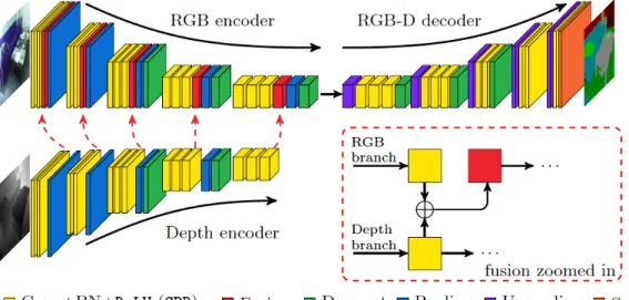
The use of CNNs with depth may also provide a way to extract better object segmen-tations, especially for objects that have similar appearances. FuseNet explores this idea by developing a network that keeps depth information in a separate channel and recombines this information throughout the neural network, as shown in Figure 2-4 [8]. Like SegNet, this network architecture is based on an encoder-decoder structure, but instead, has two encoders, one for the RGB image and one for the depth informa-tion, that are then combined before each pooling layer. This set of combined feature maps are then upsampled at the decoder. This work has shown to provide successful semantic segmentations. Consequently, this thesis aims to explore whether the ad-ditional information provided by the depth channel, particularly with regards to an object’s structure, may be able to play a role in providing better object segmentation within the oil change context.

Figure 2-4: FuseNet Architecture - The neural network layers forming FuseNet. The network takes in an RGB and depth map input and produces an object

2.5

Generative Adversarial Networks

Generative adversarial networks (GANs) are a two-model network architecture con-sisting of a generative model and a discriminative model [7]. The generative model creates samples based on features that it learns from the original data distribution. The discriminative model, on the other hand, attempts to discern between the samples created by the generative network and the original data samples, essentially acting as a classifier. Especially in cases with limited labeled data, this can improve net-work performance, as the generative model can act as an additional source of training data. In this work, we utilize the idea of GANs for semantic segmentation [16], to develop our own GAN for object segmentation, which we will refer to as SegNetGAN, as shown in Figure 2-5. With this, the generative model is the SegNet architecture, which generates predictions of object labels, while the discriminative model discerns between the ground truth training labels and the generative model predictions.

Figure 2-5: SegNetGAN Architecture - The generator-discriminator structure for SegNetGAN. The generator takes in an RGB input and produces an object segmentation at the output. The discriminator takes in ground truth or the predicted object segmentation labels and classifies the input as a real or fake label.

Chapter 3

Benchmarking Framework

This chapter describes the approach taken to perform the benchmarking analysis, including a description of the framework and the evaluation metrics. This chapter will also describe the dataset developed and used for training and evaluation, which are centered on objects commonly used in a motorcycle engine oil change task.

3.1

Framework

In this thesis, we developed benchmarking tools built upon a framework for training and testing CNNs, using PyTorch, a Python-based deep learning library, to char-acterize object segmentation and pose estimation performance on objects used in performing an autonomous oil change.

The main design goal of this framework was to make it simple and easy to develop, train, and benchmark different CNNs. The idea behind this was that the single framework would allow a variety of network architectures to be trained and tested, by simply defining the desired network architecture. In this manner, many different CNN architectures could be benchmarked easily. Moreover, we wanted to be able to benchmark a variety of metrics and incorporate new metrics effortlessly. Finally, the framework should be extensible for objects contained in any dataset. These factors inherently lead to a need for a modular and generalized design.

The main components of the framework include: a trainer, an evaluator, and a model definition. The trainer steps through the dataset for each epoch. The evaluator is used for metric computations. Finally, the model definition is used to provide a generalized structure for the developed models to inherit, including providing basic functionality such as model saving and loading.

3.2

Data

To specifically train the CNNs to detect objects relevant to the oil change task, we created our own data set consisting of scenes containing objects relative to the autonomous oil change task. To generate the data that was used for training and testing, ground truth RGB images were captured along with the corresponding depth, position, and orientation. The objects in the RGB images were also labeled. A sample of the dataset components is shown in Figure 3-1. This data was taken using a variety of different cameras and sensors including the Kinect1, Kinect2, and Xtion. Using these cameras and sensors, both RGB images and 3D point clouds were captured. These were taken in several cluttered indoor environments. At least one object of interest was included in the scene approximately 90 percent of the time. The remaining 10 percent of images were of just the background environment, with no objects of interest in the frame, to help the network discriminate between the objects of interest and clutter in the environment. Each pixel in the image was categorized with a particular object label. The pixels not corresponding to any particular object were labeled as background.

There are currently seven classes of objects to enable a robot to perform the au-tonomous motorcycle engine oil change task. These are:

Oil Bottle

1. 2. White Funnel 3. Fluid Bottle 4. Oil Filter

Funnel

(a) RGB Image (b) Object Label (c) Depth Map

(d) Orientation Label (e) Position Label

Figure 3-1: Sample Data Set Elements - The five components of the data set for a given scene, consisting of the captured RGB image and depth map, along with the

ground truth object segmentation and pose alignment labels.

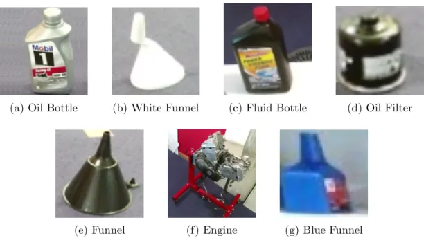
(a) Oil Bottle (b) White Funnel (c) Fluid Bottle (d) Oil Filter

(e) Funnel (f) Engine (g) Blue Funnel

Figure 3-2: Objects Classes - A sample view of each of the seven objects of interest in the data set, specific to the autonomous oil change task.

Sample images of the objects of interest are shown in Figure 3-2. While the data set is currently only specific for the seven objects in the oil change task, new objects can be added to extend the number of objects of interest in the data set for the oil change task. Moreover, new objects can also be added to target different object recognition and manipulation tasks.

The final data set is divided approximately 80/20 between training images and val-idation images, respectively. A total of 13643 images were used for training, while 2720 images were used for validation and testing. The distribution of objects for both the training and validation data sets are shown in Figure 3-3.

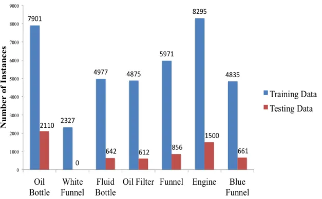
Figure 3-3: Data Set Object Distribution - This graph showcases the number of object instances in the training, as compared with the testing data set. All objects are represented in both the training and testing sets, except for the white funnel 2, with the number of object instances greater in the training data set than in the

testing data set.

2_{Because no white funnel instances are in the testing set, the results will omit the white funnel.} The white funnel was excluded, as a different funnel was ultimately used for the oil change task.

For object segmentation, both RGB images and the corresponding 3D point clouds that form a depth map of the scene were captured by the sensors. Once the RGB images were collected, the objects in approximately one-third of the images were hand labeled using LabelMe [18], while the ground truth labels for the remaining two-thirds of the images were autogenerated using a Motion Capture System.

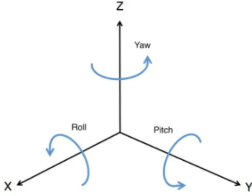
Figure 3-4: Roll Pitch Yaw Representation - A visualization of the pose representation in RPY form, with Roll, Pitch, and Yaw measured along each of the

X, Y, and Z axes, respectively.

The motion capture system also collected ground-truth pose data, consisting of both orientation and position. Position, given as the vector in Equation 3.1, contains three components, dx, dy, and dz, which are the projected distances relative to the camera

frame in each of the respective dimensions of the 3D plane. Orientation, on the other hand, is represented in Roll-Pitch-Yaw (RPY) form, which corresponds to the angle of rotation, around each of the three axes, x, y, and z, respectively, in a three dimensional plane, shown graphically in Figure 3-4, with the corresponding vector representation denoted in Equation 3.2.

P osition = (dx, dy, dz) (3.1)

OrientationRP Y = (roll, pitch, yaw) (3.2)

3.3

Training

Training was performed, with each input image in the training set accompanied by the ground truth object labels. Training was completed from scratch for all four network

architectures. The different training parameters for all of the network models are shown in Table 3.1, with the loss functions chosen such that they could be optimized using Stochastic Gradient Descent (SGD) and the learning rate tuned such that the loss converges. Training was conducted with an Nvidia Quadro M6000 GPU. The data in the training set were first scaled, such that the shortest image dimension was 244 pixels, while still maintaining the aspect ratio of the image. This scaled image was then randomly cropped to be 244 by 244 pixels, to speed up training. Data augmentation was performed on these cropped images in order to introduce additional variation in the training data by rotating the images. This data was then fed into the respective networks. For each of the networks, the training was typically run between 50 and 150 epochs, with each epoch corresponding to a full iteration through the training dataset, until the loss converged and did not decrease any further.

Model Learning Rate Loss Function

SegNet 0.001 Negative Log Likelihood (NLL) Cross Entropy Criterion

PoseNet 0.0005

Segmentation: NLL Cross Entropy Criterion

Pose: Smooth L1 Loss

SegNetGAN 0.001

Generator : NLL Cross Entropy Criterion

Discriminator : Binary Cross Entropy (BCE) Criterion

FuseNet 0.01 NLL Cross Entropy Criterion Table 3.1: Training Parameters - The learning rate and loss functions used during

training of the best model for each of the four networks. The learning rate was optimized during training for each of the network architectures.

3.4

Testing

Testing was performed on the validation set, after each training epoch, as well as after the completion of training for the saved best model based on accuracy. The data in the validation set is sent through a forward pass of the network to predict the object segmentations and pose estimations. These predictions are compared with the

ground truth labels using the evaluation metrics, as described in Section 3.5, which are computed for the entire validation set.

3.5

Benchmarking Metrics

To understand the performance of the network models, a variety of metrics are exam-ined, for both object segmentation and pose. These metrics are calculated for each individual object class and from this, an average of the metrics across all of the indi-vidual classes is computed. This was done in order to gain an overall understanding of the performance as well as how each object class factors in. Each of the metrics provides a different way of viewing how the predicted image relates to the ground truth image. In combination, the entire set of metrics provides an overall picture of the model performance that is not necessarily obtainable from just one metric.

There are four possible categories for the relation between the predicted class of a pixel and the ground truth label class: true positives (TP), true negatives (TN), false positives (FP), false negatives (FN).

With true positives, the predicted class matches the class in the ground truth label. For true negatives, a pixel that is not labeled as a given class in the ground truth is also not predicted to be of that class. In the case of false positives, or false detections, these occur when a class has been incorrectly predicted, as the ground truth is not of that class. Finally, false negatives, or missed detections, are when the ground truth is of a particular class, but that class is not predicted.

Each of these are calculated by using a confusion matrix. The confusion matrix has an entry for all possible combination of ground truth and predicted classes, where each row represents a ground truth class, while each column represents a predicted class. The entry in the corresponding row and column is incremented by one upon pixel-wise comparison between a ground truth label and a predicted image. Figure

3-5 shows a confusion matrix with the ground truth and prediction relations for a given class J , relative to class I and K.

Figure 3-5: Confusion Matrix - Relationship between Ground Truth and Prediction Labels for a Given Class J , relative to Classes I and K.

For object segmentation the four main metrics in the framework are accuracy, preci-sion, recall, and intersection over union (IOU), calculated for each class individually. Background is not considered a class in the metric calculations, since most of the pixels in an image are background, which can artificially inflate the performance, particu-larly for accuracy. By excluding background pixels, a more realistic understanding of model performance, based on just the objects of interest, can be obtained.

Accuracy reflects the number of correctly identified pixels as well as the number of correctly rejected pixels of a given class. The accuracy for a given class i is calculated using the formula in Equation 3.3:

Accuracy(i) = T P (i) + T N (i)

Precision identifies the probability that a pixel predicted to be of a given class is actually of that class. The precision for a given class i is calculated using the formula in Equation 3.4:

P recision(i) = T P (i)

T P (i) + F P (i) (3.4)

Recall is the probability that for a pixel in the ground truth label of a given class, the predicted class will match. The recall for a given class i is calculated using the formula in Equation 3.5:

Recall(i) = T P (i)

T P (i) + F N (i) (3.5)

IOU is a measure of overlap for a given class between the ground truth and prediction (intersection) divided by the sum total of predictions and ground truth labels for that given class (union). This reflects how closely the ground truth label and the predicted class label are aligned, which is critical in object segmentation. The IOU for a given class i is calculated using the formula in Equation 3.6:

IOU (i) = T P (i)

T P (i) + F P (i) + F N (i) (3.6)

To benchmark the pose estimates, pose is separated into its two components: po-sition and orientation. For each of these components, a distance metric is used to calculate the position or orientation estimation error, thereby providing a measure of the similarity between the ground truth and the predicted position or orientation, respectively. Separate distance metrics are used for calculating the position error and the orientation error in order to identify the contributions of both error sources with respect to the pose estimates for each object class. The per-class position error is calculated using Equation 3.7, where vi is the ground truth position vector

ˆ

vi is the similarly defined corresponding predicted position vector.

Errorposition(i) =

p

(vi − ˆvi) · (vi− ˆvi) (3.7)

where

vi = (dx, dy, dz) and vˆi = ( ˆdx, ˆdy, ˆdz)

The per-class orientation error is calculated similarly, but slight adaptations are made to the per-class position distance metric due to the 2π periodicity of rotation angles in order to resolve the associated ambiguities and preserve the metric in SO(3), which is defined as the set of all rotations in 3D space about the origin [9]. This modified distance metric is shown in Equation 3.8, given the ground truth orientation in RPY form as described in Equation 3.2 consisting of each of the three components, roll, pitch, and yaw, along with the corresponding predicted orientation in RPY form, similarly expressed as ˆroll, pitch, andˆ yaw.ˆ

Errororientation(i) =

q

e(roll, ˆroll)2_{+ e(pitch,pitch)}ˆ 2_{+ e(yaw, ˆyaw)}2 _(3.8)

where for any given pair (a, b):

e(a, b) = min(abs(a − b), 2π − abs(a − b))

Chapter 4

Results

The following chapter will provide a summary and analysis of the benchmarking re-sults from the experiments with SegNet, PoseNet, SegNetGAN, and FuseNet. First, the qualitative object segmentation performances of the four different models will be discussed followed by side-by-side comparison of the quantitative object segmenta-tion performance based on the metric calculasegmenta-tions of each of these four models. The performance of the networks on the robot will also be examined. Finally, both qual-itative and quantqual-itative pose estimation results obtained from PoseNet will also be detailed in this chapter.

4.1

Segmentation Results

For each of the four network architectures, data from the validation set was sampled using the best trained model to obtain the predicted segmentation results. Select instances of these results consisting of both good and poor segmentations are de-picted in this section. For each of these detailed examples, the corresponding ground truth object segmentations is also showcased in the same figure, with the top row of each figure representing the ground truth object segmentations, and the bottom row representing the predicted object segmentations. Figure 4-1 shows the segmentation results from the SegNet model, with false detections represented in Figures 4-1c and 4-1d. Similarly, the SegNetGAN model segmentation results are portrayed in Figure

4-2, with false detections in Figure 4-2c and missed detections in Figure 4-2d. Next, the segmentation results from the FuseNet model are shown in Figure 4-3. In par-ticular, false detections are shown in 4-3c, while missed detection are shown in 4-3d. Finally, Figure 4-4 depicts the segmentation results from the PoseNet model, with examples of missed detections in Figures 4-4c and 4-4d.

Ground

T

ruth

Predicted

(a) (b) (c) (d)

Figure 4-1: SegNet Segmentation Results - Correct object segmentations in 4-1a and 4-1b, with false detections in 4-1c and 4-1d.

Ground

T

ruth

Predicted

(a) (b) (c) (d)

Figure 4-2: SegNetGAN Segmentation Results - Correct object segmentations in 4-2a and 4-2b, with false detections in 4-2c and missed detections in 4-2d.

Overall, based on the segmentation results across all four models, the most prominent regions of both false and missed detections are along the edges of object boundaries.

One example of the false detections along the object boundaries is shown in Figure 4-2c. The poor segmentation at the object edge boundaries can most likely be attributed to the resolution loss in downsampling, followed by upsampling. Thus, optimizing the number of pooling layers or pooling size would likely result in better boundary segmentations, and using networks such as DilatedNet [23], which is designed to learn features at multiple scales without resolution loss, may prove promising for improving the segmentation results.

Ground

T

ruth

Predicted

(a) (b) (c) (d)

Figure 4-3: FuseNet Segmentation Results - Correct object segmentations in 4-3a and 4-3b, with false detections in 4-3c and missed detections in 4-3d.

Ground

T

ruth

Predicted

(a) (b) (c) (d)

Figure 4-4: PoseNet Segmentation Results - Correct object segmentations in 4-4a and 4-4b, with missed detections in 4-4c and 4-4d.

ap-pearance, with respect to shape and color to the actual objects of interest, are com-monly misidentified as objects of interest, since the CNN learns to associate these high-level features with the particular objects. Isolating these mistaken objects from the background, and training them as objects of interest, along with the current objects of interest, would reduce this problem.

Moreover, color was an especially important factor in the segmentation results. Ob-jects that were either black or white and reflective had higher instances of missed detections, as seen in Figures 4-4c and 4-4d with the reflective oil bottle. This inci-dence of missed detections occurs across all of the black and white objects of interest, including with the oil bottle, funnel, oil filter, and fluid bottle. The poor performance for these specific objects can be attributed to the extreme brightness or darkness of the objects that makes it harder for the correct object features to be detected.

Occlusions also impacted the segmentation performance, as the less of the objects that was visible within the camera frame, the higher the incidence of missed detections or false detections, as compared to when most of the object or the entirety of the object, was in the camera frame. The lower segmentation performance with occluded objects is related to the number of pixels needed to identify particular object features.

Additionally, the relationship between the number of pixels corresponding to an object in the camera frame and object detection is supported by the fact that for a large object, such as the engine, even when it was occluded, the segmentation was still successful, since a significant portion of the object remained, taking up a large region of pixels in the camera frame. In particular, objects that are either very close up or very far away in the camera frame were also missed more frequently, indicating that training the object at different scales would help to prevent these missed detections.

Given all of these individual factors contributing to poor segmentation, the instances of poor segmentation are often a combination of several factors. For instance,

4-1c and 4-1d are a direct result of the background objects having similar features, including shape and color, to the true objects, with occlusion also playing a role in the misidentifications. As another example, the missed detections in Figure 4-2d are due to a combination of the dark coloring of the objects, partial occlusion of the object, limiting the view of the object in the camera frame, and the rotation of the camera frame, which orients the objects in a manner that is not well represented in the training data set, despite the inclusion of data augmentation. Together, these reasons all make it difficult for the network to identify the correct features associated with the object. Furthermore, other examples of poor segmentation results, which are as a result of poor boundary edge detection, misidentifying objects of similar color and shape, and the difficulties with identifying dark colored objects are shown in Figures 4-3c and 4-3d. These poor segmentation results are further compounded as the addition of depth in FuseNet introduces additional noise into the network, degrading the object segmentation quality, particularly with black or white objects, which are difficult for the depth sensor to detect.

4.2

Segmentation Metric Comparisons

To get an overall understanding of network performance, the mean accuracy, IOU, precision, and recall values were calculated. Table 4.1 shows a comparison of the mean metric values for each of the four differing network models. Overall, PoseNet was the best performing network across the range of metrics and object classes. However, SegNetGAN and SegNet were able to outperform PoseNet in mean accuracy, while FuseNet, on the other hand, was poorest across the board, having lower performance metrics than even SegNet and SegNetGAN.

It is notable that FuseNet did not perform well, even with the incorporation of depth and in fact, performing even worse than SegNet’s object segmentation without the inclusion of depth. This is most likely due to the noise associated with the depth map, which makes it more difficult for the network to identify the objects. In particular,

small, dark colored objects, such as the fluid bottle, the oil filter, and the black funnel, for which the depth map in these regions are especially similar to the background far away, are impacted, as these regions are especially sensitive to noise. One way this could have been mitigated was through smoothing of the depth map. Moreover, the depth map was compressed from three channels, each representing an axis in the 3D plane, into only a single channel, which could have impacted the result. Therefore, keeping all three channels of the depth map separate to feed into the network archi-tecture is another way that could have provided additional information that might have improved the quality of the resulting segmentation. One final contributor to FuseNet’s poor performance may be the lack of large variability of depth informa-tion, as capturing the objects at a variety of different depths would have helped to distinguish the objects further, thus enabling the network to recognize the objects at a much higher rate.

Figure 4-5: Per Class Accuracy Figure 4-6: Per Class IOU

Figure 4-7: Per Class Recall Figure 4-8: Per Class Precision

Table 4.2 compares the individual accuracies for each class. PoseNet had the best overall accuracy with the highest accuracy scores for four of the six objects (fluid

Model Mean

Accuracy Mean IOU

Mean

Precision Mean Recall SegNet 0.972 0.730 0.912 0.783 PoseNet 0.967 0.808 0.922 0.868 SegNetGAN 0.980 0.575 0.660 0.837 FuseNet 0.957 0.322 0.469 0.524 Table 4.1: Summary of Metrics - Mean Metric Scores for all four network models, with PoseNet having the overall best performances, and FuseNet having the overall

worst performance.

bottle, oil filter, black funnel, and blue funnel). Secondly, Table 4.3 provides a com-parison between the individual IOUs for each class. PoseNet also had the best overall IOU with the highest IOU scores for the same four object classes as with accuracy. Third, a comparison of the individual precision values for each class is shown in Ta-ble 4.4. For precision, the highest precision values were split between PoseNet and SegNet, each with the highest precision score for three object classes: oil bottle, fluid bottle, and funnel versus oil filter, engine, and blue funnel, respectively. Finally, Table 4.5 compares the individual recall values for each class. For recall, PoseNet similarly had the highest recall values for the same four object classes that had the highest IOU and accuracy scores.

Model Oil Bottle

Fluid Bottle

Oil

Filter Funnel Engine

Blue Funnel SegNet 0.968 0.975 0.981 0.968 0.945 0.995 PoseNet 0.895 0.997 0.994 0.993 0.927 0.998 SegNetGAN 0.972 0.971 0.991 0.979 0.957 0.992 FuseNet 0.963 0.945 0.950 0.938 0.926 0.975 Table 4.2: Summary of Per Class Accuracy - Accuracy Scores for the classes across

all four network models, with PoseNet having the overall best accuracy.

Across these four metrics, the data implies that PoseNet produces fewer false posi-tives and missed detections, while more correctly identifying pixels corresponding to the objects of interest, as compared to any of the four network architectures investi-gated. The higher accuracy indicates that PoseNet’s more complex parallel network architecture enables the network to identify the relevant object classes correctly, as

Model Oil Bottle

Fluid Bottle

Oil

Filter Funnel Engine

Blue Funnel SegNet 0.741 0.626 0.612 0.630 0.865 0.906 PoseNet 0.523 0.896 0.816 0.865 0.819 0.930 SegNetGAN 0.728 0.576 0.527 0.555 0.837 0.801 FuseNet 0.496 0.265 0.033 0.229 0.644 0.588 Table 4.3: Summary of Per Class IOU - IOU Scores for the classes across all four

network models, with PoseNet having the overall best IOU.

the network is able to use the pose estimates to inform the object segmentation and discern between whether or not a pixel is of a given class, thereby reducing the overall missed detections and false detections.

Model Oil Bottle

Fluid Bottle

Oil

Filter Funnel Engine

Blue Funnel SegNet 0.873 0.827 0.961 0.889 0.950 0.970 PoseNet 0.910 0.928 0.883 0.901 0.948 0.959 SegNetGAN 0.820 0.780 0.602 0.612 0.898 0.905 FuseNet 0.565 0.547 0.280 0.341 0.688 0.861 Table 4.4: Summary of Per Class Precision - Precision Scores for the classes across all four network models, with PoseNet and SegNet having the overall best precision.

However, the parallel architecture is also the reason why PoseNet did not have the highest metric scores for all of the object classes among the four network architec-tures, since any poor pose estimates would contribute to and result in the poor ob-ject segmentation performance. Consequently, although PoseNet had the best overall performance, SegNet and SegNetGAN outperformed PoseNet on the four metrics, particularly with respect to the oil bottle and engine. With the oil bottle and the engine, SegNetGAN had the highest accuracy and recall values, while SegNet had the highest IOU values for these two object classes and the highest precision for the engine. These results are likely due to the fact that because the oil bottle is reflec-tive and nearly symmetric, while the engine is large, and therefore occluded in many scenes, resulting in poor pose estimates from PoseNet, and as a result poor object segmentations. In contrast, SegNet and SegNetGAN are more adept at handling the

difficulties associated with the oil bottle and the engine resulting in higher perfor-mances for these objects. With SegNetGAN, the generator in SegNetGAN essentially creates additional training data, helping the network to be able to better learn the features associated with an object. The improved learning allows the network to identify the relevant objects at a higher rate, leading to fewer missed detections and resulting in higher recall and accuracy scores, particularly with objects, such as the oil bottle and engine, that are not easily detected. With SegNet, it is able to perform more consistently across all objects, including the oil bottle and the engine, since SegNet is designed specifically for object segmentation.

Model Oil Bottle

Fluid Bottle

Oil

Filter Funnel Engine

Blue Funnel SegNet 0.831 0.721 0.628 0.683 0.906 0.932 PoseNet 0.552 0.962 0.915 0.955 0.858 0.968 SegNetGAN 0.867 0.688 0.810 0.857 0.924 0.874 FuseNet 0.803 0.340 0.036 0.409 0.909 0.650 Table 4.5: Summary of Per Class Recall - Recall Scores for the classes across all four

network models, with PoseNet having the overall best recall.

Overall, based on the comparison of the metric results, IOU has shown to be the most informative metric, due to the fact that both false detections and missed detections are taken into account in the metric computation, instead of only one or the other, as in the case with precision and recall. On the other hand, accuracy is less informative, as the true negatives account for a large number of pixels. Consequently, the accuracy calculation can become inflated, which can be seen by the high scores with very little deviation, across all of the object classes and network architectures.

Furthermore, as a general trend across all four metrics and four networks, certain object classes performed better than others. The engine had overall high performance due to its large, distinct shape and highly detailed appearance. The blue funnel also tended to have high performance due to its uniqueness in color and shape. The oil bottle had some instances of lower performance, as a result of not only its reflective

surface, but also because of its similar appearance to other objects in the background. Finally, the funnel, oil filter, and fluid bottle, all had performance issues due to their black coloring, as other black objects were also present in the background, causing the background to be falsely detected.

4.3

Robot Performance Comparisons

The networks investigated were fed directly through the robot perception pipeline to determine the segmentation performance between the different models on the robot itself. The visualization in Figure 4-9 shows a screenshot of the predicted object segmentations that the robot sees for each given model. These predicted segmenta-tions give an indication of how well these models work in a live setting, as another method of evaluating the models, beyond the validation dataset. Figure 4-9a shows the original image view from the robot. The remaining figures showcase the object segmentations as an overlay on top of the original image for each of the given net-work models. Figure 4-9b is the visualization with the SegNet model; Figure 4-9c is the visualization with the PoseNet model; Figure 4-9d is the visualization with the SegNetGAN model; and Figure 4-9e is the visualization with the FuseNet model.

Comparing the performances from these results, the SegNetGAN model performed the best, as it was able to segment the three objects entirely without false detections. SegNet performed slightly worse, as there were some false detections along the edge of the blue funnel. Moreover, only a very small region of the oil bottle was detected, while the bottom part of the engine was not detected. FuseNet performed worse than both SegNetGAN and SegNet. Although there were only minimal false detections along the blue funnel boundaries, the oil bottle was not detected at all, and regions along the engine edges were missed. The worst performing network was PoseNet. The oil bottle was not detected at all. Instead part of the oil bottle, along with the neighboring region on the black cloth, is falsely identified as the blue funnel. Additionally, only some of the engine is detected. Of the three objects in the scene,

PoseNet was most successful in detecting the blue funnel, correctly identifying a majority of the blue funnel, but even this detection was less successful when compared to the SegNetGAN, FuseNet or SegNet blue funnel detections, which were able to encompass more of the entire blue funnel area.

(a) Original Image (b) SegNet Robot Results (c) PoseNet Robot Results

(d) SegNetGAN Robot Results (e) FuseNet Robot Results

Figure 4-9: Robot Performance Comparisons - A comparison of the performance of a scene from the robot’s point of view based on the predicted object segmentations

for each of the four different network architectures.

Although the performance of each of the networks on the robot is not exactly consis-tent with the numerical metric data, there are a number of factors that could cause this discrepancy in performance. For one, the metrics may not provide a good corre-lation to robot performance. Even though both missed detections and false positives are important factors to consider when testing performance on a robot, because on one hand, detections are necessary for any object manipulation with the robot, while on the other hand, minimizing the false detections will allow for better segmentation fits with the point cloud model, these may not be the only performance measures to consider. Moreover, the differences in lighting conditions between the validation set and the view from the robot may also play a role. The view from the camera is actually brighter than the training and validation images. Having the brighter images

improved SegNetGAN segmentation on the robot, as SegNetGAN routinely missed the darker, black objects, such as the oil filter, but was able to detect the brighter and more reflective objects, like the oil bottle, in the validation set. However, Seg-Net, FuseNet and PoseNet all exhibited some poor performance with the reflective oil bottle in the validation set, explaining the poorer performance when tested on the robot. This is explained by the fact that with SegNetGAN, noise is introduced into the network, which improves the robustness of detection for the lighter objects.

4.4

PoseNet Pose Estimation Results

In addition to object segmentation, this thesis performed benchmarking on pose es-timates generated by PoseNet. Preliminary results from this benchmarking are pre-sented below. Quantitatively, there were discrepancies between the estimated and ground truth pose for all object classes in both orientation and position, as reflected by Table 4.6, which shows the average orientation error in radians and position error in meters for each of the object classes. Across all classes, the average position error is 0.332 meters, while the average orientation error is 0.657 radians or approximately 38 degrees. Looking at the classes individually, the largest position error was with the engine, while the smallest position error was with the oil filter. These results correlate to the scale of the objects, given the engine as the largest object, and the oil filter as the smallest object in the data set, which take up more or less area in the camera frame, respectively, indicating the position error is proportional to the size of the object in the camera frame. On the other hand, the largest orientation error was with the oil bottle, while the oil filter had the smallest orientation error. The orientation error is likely due to object symmetry, since several different object orientations can have the same learned visual features. While the oil filter is only symmetric along a single axis, the oil bottle is nearly symmetric along multiple axes, resulting in the larger error for the oil bottle.

visible qualitatively, as shown in Figure 4-10, which is a set of sample pose estimates from the validation set using the best trained PoseNet model. The top row represents the ground truth pose projected into the frame, while the bottom row represents the projection given the predicted pose. This projection takes both orientation and position relative to the camera view into account.

Oil Bottle

Fluid Bottle

Oil

Filter Funnel Engine

Blue Funnel Position Error (meters) 0.270 0.247 0.215 0.436 0.548 0.432 Orientation Error (radians) 1.523 0.527 0.392 0.834 0.494 0.629 Table 4.6: Summary of Per Class Orientation and Position Distance - Position and

Orientation Distance Scores for PoseNet across all four network models.

In Figures 4-10a through 4-10d, all of the objects are shifted or rotated from their ground truth positions and orientations, except for the engine in Figure 4-10a. Similar to the quantitative findings, for position, the objects that took up a smaller portion of the scene were able to produce position estimates that were closer to the ground truth position, since the error does not propagate as much for smaller deviations in position. With orientation, there is variation between the estimated and ground truth values, but the most drastic difference in object orientation can be seen with the oil bottle, which is rotated 180 degrees and the oil filter which is rotated 90 degrees, as shown in Figures 4-10c and 4-10d, respectively. This error in the orientation estimate can be attributed to the difficulties in determining the orientation of objects that are symmetric, since there are no significant visual differences, regardless of the object orientation. By addressing the reason behind the poor pose estimates, the error can be reduced, thereby improving the pose estimations. This improvement, in turn, may improve PoseNet object segmentations, since poor pose estimates yields poor object segmentations, as pose estimates and object segmentations are intertwined through the PoseNet architecture.

Ground

T

ruth

Predicted

(a) (b) (c) (d)

Figure 4-10: PoseNet Pose Projection Results - Discrepancies exist between ground truth and predicted pose in all samples, including 4-10a and 4-10b, except for engine pose estimate in 4-10a. The largest discrepancies are with pose estimate for

oil bottle and oil filter, respectively in 4-10c and 4-10d.

Overall, the error in both the position and orientation pose estimates indicates that PoseNet was not able to regress either the orientation or position effectively. Several factors may have contributed to these poor results. For one, the processing of the pose data could potentially be affecting the results, particularly the representation of orientation in RPY. Another orientation representation, such as quaternions, could improve the results, as this eliminates the possibility that rotating along one axis results in the other two rotational axes pointing in the same direction. As another contributing factor, the single regression layer used in the pose estimation branch of PoseNet could have been too limited to be able to produce pose estimates with low error. Adding additional layers to the pose estimation branch may also lead to improvements in the pose estimates. Finally, since no constraints are applied to join the position estimate and the predicted object segmentation, applying this constraint could produce smaller position error.

Chapter 5

Conclusions

This chapter will highlight and summarize the main points of this research, including the results in Chapter 4. It will also discuss gaps remaining in the research as possible directions for further work to be done in the future.

5.1

Summary

In this thesis, four different CNNs, SegNet, SegNetGAN, PoseNet, and FuseNet, were investigated and benchmarked to compare their performance with regards to object segmentation. In addition, the pose estimates generated by PoseNet were also benchmarked. Specifically, this thesis provides a framework for these networks to be compared with one another in a simple and objective manner. SegNet was the foun-dational network tested in this thesis. The remaining three networks, SegNetGAN, PoseNet, and FuseNet are all built upon SegNet. All four networks takes in RGB input and produces object segmentations at the output, with FuseNet also taking in depth as input, PoseNet also producing pose estimations along with the object segmentations, and SegNetGAN also differentiates between predicted object segmen-tations and ground truth object segmensegmen-tations. Overall, this work shows that all four of the differing network architectures are able to perform object segmentation. In fact, we were able to show some improvements in object segmentation over SegNet through the use of differing network architectures. While more complicated network